


1. Introduction
The study of micron-scale self-propelled objects such as bacteria, algae and synthetic Janus particles has become a dynamic field of research, both for the motion of individual bodies (Lauga & Powers Reference Lauga and Powers2009) and for the collective behaviour of suspensions of active particles (Ramaswamy Reference Ramaswamy2010; Marchetti et al. Reference Marchetti, Joanny, Ramaswamy, Liverpool, Prost, Rao and Simha2013; Bechinger et al. Reference Bechinger, Di Leonardo, Löwen, Reichhardt, Volpe and Volpe2016; Gomper et al. Reference Gomper2020). Owing to the particles’ self-motion, active matter can spontaneously phase-separate into dense and dilute regions (Cates et al. Reference Cates, Marenduzzo, Pagonabarraga and Tailleur2010; Fily & Marchetti Reference Fily and Marchetti2012; Bialké, Löwen & Speck Reference Bialké, Löwen and Speck2013; Buttinoni et al. Reference Buttinoni, Bialké, Kümmel, Löwen, Bechinger and Speck2013; Palacci et al. Reference Palacci, Sacanna, Steinberg, Pine and Chaikin2013; Stenhammar et al. Reference Stenhammar, Tiribocchi, Allen, Marenduzzo and Cates2013; Takatori, Yan & Brady Reference Takatori, Yan and Brady2014; Wysocki, Winkler & Gompper Reference Wysocki, Winkler and Gompper2014; Takatori & Brady Reference Takatori and Brady2015; Digregorio et al. Reference Digregorio, Levis, Suma, Cugliandolo, Gonnella and Pagonabarraga2018) and can move collectively under an orienting field (Takatori & Brady Reference Takatori and Brady2014). Active particles can also be harnessed to do work, for example by turning a micro-gear (Angelani, Costanzo & Di Leonardo Reference Angelani, Costanzo and Di Leonardo2011), or can flow spontaneously in a channel without an applied pressure difference (Lushi, Goldstein & Shelley Reference Lushi, Goldstein and Shelley2012; Guo et al. Reference Guo, Samanta, Peng, Xu and Cheng2018). It has also been observed in simulations and experiments that a passive object with an asymmetric shape can achieve net directed motion in a bath of active particles (Kaiser et al. Reference Kaiser, Sokolov, Aranson and Löwen2015).
Directed motion in a bath of passive particles, e.g. a chemical solute, is also possible when there is a concentration gradient of bath particles, a phenomenon known as diffusiophoresis. To achieve diffusiophoretic motion, not only must there be a concentration gradient, but there must also be an interactive force between the larger phoretic particle and the smaller ‘bath’ or solute particles. The interactive force couples with the concentration gradient to drive a hydrodynamic flow adjacent to the phoretic particle surface, and the phoretic particle, being force-free, moves in response to the combined shear and interactive force. The system is out of equilibrium owing to the imposed concentration gradient. In classical diffusiophoresis, a uniform macroscopic concentration gradient is maintained by some external means (Anderson Reference Anderson1989). More recent examples concern self-diffusiophoresis where a chemical reaction occurs asymmetrically on the particle surface, leading to a local concentration gradient that drives the phoretic motion (Paxton et al. Reference Paxton, Kistler, Olmeda, Sen, St. Angelo, Cao, Mallouk, Lammert and Crespi2004; Howse et al. Reference Howse, Jones, Ryan, Gough, Vafabakhsh and Golestanian2007; Córdova-Figueroa & Brady Reference Córdova-Figueroa and Brady2008; Brady Reference Brady2011).
Passive, Brownian or solute, particles are characterized by their thermal diffusivity given by the Stokes–Einstein–Sutherland relation:  $D_T = k_BT/\zeta$, where
  $k_BT$ is the thermal energy and
  $\zeta = 6 {\rm \pi}\eta a$ is the Stokes drag coefficient of a Brownian particle of size
  $a$ in a fluid of viscosity
  $\eta$. When interacting with a larger phoretic particle of size
  $R$ through a short-range repulsive interactive force with characteristic length scale
  $b$ and an imposed concentration gradient
  $\boldsymbol {\nabla } n$, the passive bath particles drive the phoretic particle with the well-known velocity
 \begin{equation} \boldsymbol{U}^{passive} ={-} \frac{1}{2} b^2 \frac{k_BT}{\eta} \boldsymbol{\nabla} n , \end{equation}
where  $n$ is the number density of bath particles (see § 2 and (2.34)). This phoretic velocity is independent of the size of the phoretic particle (and of the Brownian bath particles). Because of the assumed repulsive interactions, the motion is from regions of high concentration to low – the phoretic particle lowers its free energy by moving to regions with fewer unfavourable interactions. For attractive interactions the motion is in the opposite direction.
The main question we wish to address in this work is: What diffusiophoretic motion occurs in a bath of active particles?
The simplest description of active particles is the so-called active Brownian particle (ABP) model where, in addition to normal thermal Brownian motion with diffusivity  $D_T$, the particles self-propel with a ‘swim’ velocity
  $U_0$ in a direction
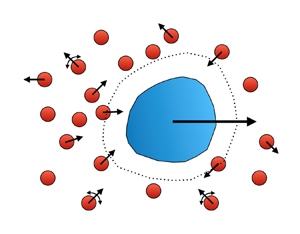
  $\boldsymbol {q}$, as illustrated in figure 1. The orientation of the swimming direction changes on a reorientation time scale
  $\tau _R$ that results from either random Brownian rotations or from the run-and-tumble behaviour often observed with bacteria. The ABPs take a step of magnitude
  $\ell = U_0 \tau _R$, which defines the run length
  $\ell$, and at long times undergo a random walk with a ‘swim diffusivity’
  $\boldsymbol {D}^{swim} = (U_0\ell /6) \boldsymbol {I}$ in three dimensions. In analogy with the Stokes–Einstein–Sutherland relation, we can define an ‘energy’ scale for active matter via
  $D^{swim} = k_sT_s/\zeta$, and thus define the ‘activity’
  $k_sT_s = \zeta U_0 \ell /6$ (Takatori & Brady Reference Takatori and Brady2015). An important parameter then is the relative importance of the activity to thermal energy,
  $k_sT_s/k_BT = D^{swim}/D_T$. In many active matter systems this ratio can easily exceed
  $10^3$ (Takatori et al. Reference Takatori, De Dier, Vermant and Brady2016).

Figure 1. A large particle of size  $R$ is immersed in a bath of smaller colloidal particles of size
  $a$. Each bath particle has thermal diffusivity
  $D_T$ and can be active and self-propel with a swim speed
  $U_0$ in the direction
  $\boldsymbol {q}$ that reorients on the time scale
  $\tau _R$. The bath particles interact with the large particle via an interparticle force
  $\boldsymbol {f}_p$ at a characteristic distance
  $b$ from the particle surface. A concentration gradient of bath particles can result in motion of the large particle with a phoretic velocity
  $\boldsymbol {U}$.
We show by explicit calculation that in the high-activity limit,  $k_sT_s/k_BT \gg 1$, the classic phoretic velocity (1.1) becomes
 \begin{equation} \boldsymbol{U}^{active} ={-} \frac{1}{3} b^2 \frac{k_sT_s}{\eta} \boldsymbol{\nabla} n , \end{equation}
where the activity  $k_sT_s$ replaces the thermal energy
  $k_BT$. Note, however, that it is not a simple replacement; the coefficient in front is different,
  $1/3$ versus
  $1/2$. While the form (1.2) has a natural appeal and also shows the independence of the size
  $R$ of the phoretic particle, from the definition of the activity
  $k_sT_s$ (1.2) may be better understood as
 \begin{equation} \boldsymbol{U}^{active} ={-} U_0 \ell \boldsymbol{\nabla} \phi_b . \end{equation}
For active matter, the phoretic velocity is proportional to the swim speed  $U_0$, the run length
  $\ell = U_0 \tau _R$ and the gradient in the ‘volume’ fraction of ABPs,
  $\phi _b = b^2 a {\rm \pi}n/3$. Note, importantly, that it is now independent of the viscosity of the suspending fluid as both the propulsive swim force of the ABPs,
  $\zeta U_0 \boldsymbol {q}$, and the viscous drag of the phoretic particle,
  $6{\rm \pi} \eta R\, \boldsymbol {U}$, are proportional to the viscosity; this should be familiar from the swimming behaviour of micro-organisms, which is also independent of the fluid viscosity. Interestingly, at high activity the phoretic motion is always down the concentration gradient even if there are favourable interactions between the phoretic particle and the active bath particles (see § 4).
Since active matter is inherently out of equilibrium, there are other mechanisms for phoretic motion that do not require a concentration gradient. When the run length varies with spatial position,  $\ell (\boldsymbol {x})$, net phoretic motion can occur. A spatially dependent run length can result because the reorientation time,
  $\tau _R(\boldsymbol {x})$, varies, and/or because the swim speed varies with position,
  $U_0(\boldsymbol {x})$. These variations may arise from a spatially varying fuel source or a chemoattractant that affects the swim speed/reorientation time, or certain bacteria and synthetic swimmers can be light-activated, allowing control of swim speed and direction. In § 3.2 we show that at high activity the phoretic velocity is given by
 \begin{equation} \boldsymbol{U}^{active} ={-} \phi_b U_0 \boldsymbol{\nabla} \ell . \end{equation}
And we show further that (1.2)–(1.4) are special cases of the more general high-activity form
 \begin{equation} \boldsymbol{U}^{active} ={-} \frac{1}{3} \frac{b^2}{\eta}\boldsymbol{\nabla} \varPi^{swim} , \end{equation}
where  $\varPi ^{swim} = n k_sT_s = n \zeta D^{swim}$ is the swim pressure (Takatori et al. Reference Takatori, Yan and Brady2014).
A physical explanation for the swim pressure gradient as the driving force for phoretic motion is the following. Each ABP exerts its swim force of magnitude  $\zeta U_0$ when contacting the phoretic particle. An active bath particle must be within a run length
  $\ell$ of the phoretic particle surface in order to hit it, and thus the number of bath particles that strike the phoretic particle scales as
  $4{\rm \pi} R^2 \ell n$. A net force results from the change from one side to the other,
  $F^{net} \sim \varDelta ( \zeta U_0 4{\rm \pi} R^2 \ell n ) \sim 4{\rm \pi} R^2 \Delta \varPi ^{swim} \sim 4 {\rm \pi}R^3\boldsymbol {\nabla } \varPi ^{swim}$. This force is reduced in magnitude by
  $(b/R)^2$ owing to the hydrodynamic flow adjacent to the phoretic particle (see § 2), and is balanced by the Stokes drag,
  $-6{\rm \pi} \eta R U$, to give the phoretic velocity (1.5).
The result (1.4) predicts a surprising phenomenon: a spatially varying run length can lead to a reverse phoretic effect in which the particle moves towards regions of higher bulk active bath particle concentration even though it is repelled by the ABPs.
It is interesting to note that for passive Brownian bath particles, when there is a spatial variation in the temperature  $T$ in addition to concentration, the motion of the colloidal particle is also given by the form (1.5) but with the osmotic pressure
  $\varPi ^{osm} = nk_BT$ replacing
  $\varPi ^{swim}$ (Dhont Reference Dhont2004).
Finally, we consider a field that biases the orientation of the ABPs but does not propel them. The phoretic velocity is
 \begin{equation} \boldsymbol{U}^{active} ={-} \phi_b U_0 \ell \boldsymbol{\nabla} \varPsi , \end{equation}
where  $\varPsi$ is a non-dimensional ‘potential’ that has the form
  $- \hat {\boldsymbol {H}} \boldsymbol {\cdot }\boldsymbol {x}/\ell$ for an orienting field with direction the unit vector
  $\hat {\boldsymbol {H}}$. Indeed, all three mechanisms for phoretic motion can be written in the form (1.6) with the ‘potential’ being
  $+ \ln n$ for a concentration gradient and
  $+\ln \ell$ for spatially varying activity.
To obtain the results for phoretic motion, in § 2 we derive a new formulation and perspective that is applicable to both passive and active systems. This development is at the ‘continuum’ level, where the phoretic particle is large compared with the size of the bath particles so that we can model the bath as a suspension. By recognizing that the suspension stress is composed of two contributions, the usual Newtonian fluid stress and a contribution from the bath particles, we use the reciprocal theorem for Stokes flow to write the hydrodynamic force on the phoretic particle as a composition of two parts: (i) the drag force  $- \boldsymbol {R}_{FU} \boldsymbol {\cdot } \boldsymbol {U}$ for translating the particle with velocity
  $\boldsymbol {U}$, where
  $\boldsymbol {R}_{FU}$ the well-known hydrodynamic resistance tensor coupling the force and the velocity, and (ii) a ‘propulsive’ or thrust force that can be expressed as a volume integral of the fluid velocity field generated by translating the particle times the sum of the divergence of the non-hydrodynamic stress tensor and the interactive force between the bath and the phoretic particle (see (2.13)). This formulation is similar to treatments of the swimming of micro-organisms (Stone & Samuel Reference Stone and Samuel1996; Swan et al. Reference Swan, Brady and Moore2011) and applies to bodies of any shape and to any form of the interactive force between the bath and phoretic particle.
From this perspective we show that when the interactive force is short-ranged and repulsive, the local osmotic pressure of the bath particles,  $\varPi ^{osm} = n k_BT$, drives a ‘slip’ velocity adjacent to the phoretic particle surface, which then moves so as to satisfy the constraint of no net force on the phoretic particle. The result for a spherical phoretic particle is then the classical expression (1.1). The behaviour for passive particles in § 2 is generalized to have any form and range of interactive force.
Owing to their persistent motion, active particles accumulate at no-flux surfaces, and at high activity there is a thin accumulation boundary layer in which the surface concentration is  $n^{out} k_sT_s/k_BT$, where
  $n^{out}$ is the concentration just outside the accumulation boundary layer (Yan & Brady Reference Yan and Brady2015). The local osmotic pressure is replaced by the swim pressure
  $\varPi ^{swim} = n^{out}k_sT_s$ and (1.2) follows for motion driven by a bulk concentration gradient, as we show by detailed calculation in § 3. Also in § 3 we show that motions due to a concentration gradient and to a spatially varying run length (spatially varying activity) are both expressible in terms of the gradient in the swim pressure (1.5).
Finally, we conclude in § 4 with a discussion of the limitations and extensions of this treatment of phoretic motion for passive and active bath particles, and of its use for other microstructured fluids such as nematic or polymeric fluids.
2. Phoretic motion in a bath of passive particles
Consider a ‘phoretic’ particle of characteristic size  $R$ immersed in a fluid containing a dilute suspension of colloidal bath particles of characteristic size
  $a$, as illustrated in figure 1. We take a ‘continuum’ perspective by which we mean that a volume element of size
  $\delta V$ exists that contains a sufficient number of bath particles to form a continuum:
  $a \ll (\delta V)^{1/3} \ll R$. The number density of bath particles at the ‘continuum point’ is
  $n(\boldsymbol {x},t)$. The continuum momentum balance for the suspension – the mixture of fluid plus particles – is
 \begin{equation} \rho \frac{\textrm{D} \boldsymbol{u}}{\textrm{D}t} = \boldsymbol{\nabla} \boldsymbol{\cdot} {\boldsymbol{\sigma}} + n \boldsymbol{f}_p, \quad \boldsymbol{\nabla} \boldsymbol{\cdot} \boldsymbol{u} = 0 , \end{equation}
where  $\rho$ is the mass density of the suspension,
  $\boldsymbol {u}$ is the suspension average velocity,
  ${\boldsymbol {\sigma }}$ is the suspension stress and
  $\boldsymbol {f}_p$ is the interactive force exerted on a bath particle by the larger phoretic particle.
The continuum and interactive force and torque exerted on the phoretic particle are
 $$\begin{gather} \boldsymbol{F} = \oint_{S_P} {\boldsymbol{\sigma}}\boldsymbol{\cdot} \boldsymbol{n} \, \textrm{d}S - \int_{V_f} n\boldsymbol{f}_p \, \textrm{d}V , \end{gather}$$
 $$\begin{gather}\boldsymbol{L} = \oint_{S_P}\boldsymbol{r} \times {\boldsymbol{\sigma}}\boldsymbol{\cdot} \boldsymbol{n} \, \textrm{d}S - \int_{V_f} \boldsymbol{r} \times n \boldsymbol{f}_p \, \textrm{d}V , \end{gather}$$
where each bath particle exerts the force  $-\boldsymbol {f}_p$ on the phoretic particle,
  $\boldsymbol {n}$ is the outer normal to the phoretic particle surface,
  $\boldsymbol {r}$ is measured relative to the phoretic particle ‘centre’ and we have assumed that the torques arise only from force moments. The volume integral is over the fluid volume exterior to the phoretic particle.
The motion of the phoretic particle follows from the force and torque balances
 $$\begin{gather} m\frac{\textrm{d}\boldsymbol{U}}{\textrm{d}t} = \boldsymbol{F} + \boldsymbol{F}^{ext} , \end{gather}$$
 $$\begin{gather}\frac{\textrm{d}}{\textrm{d}t}(\boldsymbol{M} \boldsymbol{\cdot}\boldsymbol{\varOmega}) = \boldsymbol{L} + \boldsymbol{L}^{ext} , \end{gather}$$
where  $m$ and
  $\boldsymbol {M}$ are the particle's mass and moment of inertia, and
  $\boldsymbol {F}^{ext}$ and
  $\boldsymbol {L}^{ext}$ are any external forces or torques exerted on the phoretic particle; e.g. an external gravitational force would be
  $\boldsymbol {F}^{ext} = (m - \rho V_R) \boldsymbol {g}$, where
  $V_R$ is the volume of the phoretic particle.
We are primarily interested in the motion of small particles such that the acceleration of both the suspension and the phoretic particle are negligible. In this low-Reynolds-number limit, the definition of phoretic motion is that there is no external force/torque on the particle; thus, from (2.4) and (2.5),  $\boldsymbol {F} = 0$ and
  $\boldsymbol {L} = 0$.
In order to make the presentation as clear as possible, in going forward we will not discuss the torque balance on the phoretic particle. The full detailed expressions including the torque are given in Appendix A.
The constitutive law for the suspension stress is composed of two terms,
 \begin{equation} {\boldsymbol{\sigma}} = {\boldsymbol{\sigma}}_f + {\boldsymbol{\sigma}}_p , \end{equation}
where the fluid stress tensor is  ${\boldsymbol {\sigma }}_f = - p_f \boldsymbol {I} + 2 \eta \boldsymbol {e}$, with
  $p_f$ the pressure in the fluid,
  $\eta$ the shear viscosity and
  $\boldsymbol {e}$ the rate of strain tensor of the suspension velocity
  $\boldsymbol {u}$, and the contribution from the bath particles is
  ${\boldsymbol {\sigma }}_p$, whose form is specified below.
The bath particle number density satisfies the usual conservation equation
 \begin{equation} \frac{\partial n}{\partial t} + \boldsymbol{\nabla} \boldsymbol{\cdot} \boldsymbol{j} = 0 , \end{equation}
where  $\boldsymbol {j}$ is the flux of bath particles. The boundary condition at the phoretic particle surface would be either no net flux,
  $\boldsymbol {n}\boldsymbol {\cdot } \boldsymbol {j} = 0$, or a net rate of production/consumption due to a chemical reaction for self-propelled catalytic motors,
  $\boldsymbol {n}\boldsymbol {\cdot } \boldsymbol {j} = \mbox {rxn}$ (Paxton et al. Reference Paxton, Kistler, Olmeda, Sen, St. Angelo, Cao, Mallouk, Lammert and Crespi2004; Howse et al. Reference Howse, Jones, Ryan, Gough, Vafabakhsh and Golestanian2007; Córdova-Figueroa & Brady Reference Córdova-Figueroa and Brady2008; Brady Reference Brady2011).
In the absence of the phoretic particle, there is a given distribution of bath particles  $n^\infty (\boldsymbol {x},t)$, the associated bath particle flux
  $\boldsymbol {j}^\infty$, and fluid motion and stress fields
  $\boldsymbol {u}^\infty$ and
  ${\boldsymbol {\sigma }}^\infty$. These fields satisfy the conservation equations in the absence of the phoretic particle:
  $\boldsymbol {\nabla }\boldsymbol {\cdot } {\boldsymbol {\sigma }}^\infty = 0$,
  $\boldsymbol {\nabla } \boldsymbol {\cdot } \boldsymbol {u}^\infty = 0$ and
  $\partial n^\infty /\partial t + \boldsymbol {\nabla } \boldsymbol {\cdot } \boldsymbol {j}^\infty = 0$. For example, we might have an imposed concentration gradient of bath, or solute, particles:
  $n^\infty (\boldsymbol {x}, t) = \boldsymbol {x} \boldsymbol {\cdot } \boldsymbol {\nabla } n^{ext}$, with constant concentration gradient
  $\boldsymbol {\nabla } n^{ext}$. We could also have a constant flow at infinity, e.g.
  $\boldsymbol {u}^\infty = \boldsymbol {U}^\infty$. What is relevant for the motion of the phoretic particle is the departure from this ‘far-field’ distribution – the disturbance problem – which takes the form
 $$\begin{gather} \boldsymbol{\nabla}\boldsymbol{\cdot}{\boldsymbol{\sigma}}_f^\prime ={-} \boldsymbol{\nabla }\boldsymbol{\cdot} {\boldsymbol{\sigma}}_p^\prime - (n^\prime + n^\infty)\boldsymbol{f}_p , \end{gather}$$
 $$\begin{gather}\boldsymbol{\nabla} \boldsymbol{\cdot} \boldsymbol{u}^\prime = 0, \end{gather}$$
 $$\begin{gather}p_f^\prime , \boldsymbol{u}^\prime \sim 0 \quad \mbox{as} \ r \rightarrow \infty , \end{gather}$$
 $$\begin{gather}\boldsymbol{u}^\prime = \boldsymbol{U} - \boldsymbol{U}^\infty \quad \mbox{on} \ S_P , \end{gather}$$
where  $\boldsymbol {U}$ is the unknown translational velocity of the phoretic particle to be found from the force balance on the particle. Since the ‘field at infinity’ does not exert any net force,
 \begin{equation} \boldsymbol{F} = \oint_{S_P} {\boldsymbol{\sigma}}_f^\prime\boldsymbol{\cdot} \boldsymbol{n} \, \textrm{d}S + \oint_{S_P} {\boldsymbol{\sigma}}_p^\prime\boldsymbol{\cdot} \boldsymbol{n} \, \textrm{d}S- \int_{V_f} (n^\prime + n^\infty)\boldsymbol{f}_p \, \textrm{d}V . \\ \end{equation}
The interactive force only exists because of the phoretic particle, and thus the ‘disturbance quantity’  $n^\infty \boldsymbol {f}_p$ appears in (2.8) and (2.12). (We also assume that the interactive force
  $\boldsymbol {f}_p$ and particle stress
  ${\boldsymbol {\sigma }}_p^\prime$ decay sufficiently fast that all integrals are convergent.)
We can make use of the reciprocal theorem for Stokes flow to bypass the determination of the velocity and stress fields in (2.8) and compute directly the hydrodynamic force,  $\oint _{S_P} {\boldsymbol {\sigma }}_f^\prime \boldsymbol {\cdot } \boldsymbol {n} \, \textrm {d}S$, on the particle. For any body shape, the hydrodynamic force is given by
 \begin{equation} \oint_{S_P} {\boldsymbol{\sigma}}_f^\prime\boldsymbol{\cdot} \boldsymbol{n} \, \textrm{d}S ={-} \boldsymbol{R}_{FU} \boldsymbol{\cdot}(\boldsymbol{U} - \boldsymbol{U}^\infty) + \int_{V_f} \boldsymbol{{\mathcal{U}}}_U\boldsymbol{\cdot} ( \boldsymbol{\nabla} \boldsymbol{\cdot} {\boldsymbol{\sigma}}_p^\prime + n\boldsymbol{f}_p) \, \textrm{d}V , \end{equation}
where we have used the total concentration  $n = n^\prime + n^\infty$. Here,
  $\boldsymbol {R}_{FU}$ is the hydrodynamic resistance tensor coupling the force to the velocity for the given phoretic particle body geometry and
  $\boldsymbol {{\mathcal {U}}}_U$ is a second-order tensor field that gives the fluid velocity at any point outside the particle when it translates with a constant velocity of unit magnitude. (When there is translational–rotational coupling, i.e. chiral particles, the torque balance is also necessary as discussed in Appendix A.) For example, for a spherical particle of radius
  $R$ the resistance tensor is isotropic and given by
  $\boldsymbol {R}_{FU} = 6{\rm \pi} \eta R \boldsymbol {I}$, while the second-order tensor velocity field outside the sphere is
 \begin{equation} \boldsymbol{{\mathcal{U}}}_U = \frac{3}{4}\left( \frac{\boldsymbol{I}}{r} + \frac{\boldsymbol{r}\boldsymbol{r}}{r^3}\right) + \frac{1}{4}\left(\frac{\boldsymbol{I}}{r^3} - \frac{3\boldsymbol{r}\boldsymbol{r}}{r^5}\right) \, , \end{equation}
where  $\boldsymbol {r}$ has been scaled with the particle radius
  $R$.
$R$.
Combining the expression (2.13) for the hydrodynamic force with the remaining terms in (2.12) and making use of the divergence theorem for  ${\boldsymbol {\sigma }}_p^\prime$, we have for the phoretic velocity of the particle
 \begin{equation} \boldsymbol{U} - \boldsymbol{U}^\infty = \boldsymbol{R}_{FU}^{{-}1} \boldsymbol{\cdot} \int_{V_f} (\boldsymbol{{\mathcal{U}}}_U - \boldsymbol{I}) \boldsymbol{\cdot} \boldsymbol{\nabla}\boldsymbol{\cdot}{\boldsymbol{\sigma}}_p^\prime \, \textrm{d}V + \boldsymbol{R}_{FU}^{{-}1} \boldsymbol{\cdot} \int_{V_f} (\boldsymbol{{\mathcal{U}}}_U - \boldsymbol{I}) \boldsymbol{\cdot} n \boldsymbol{f}_p \, \textrm{d}V . \end{equation}
Equation (2.15) for the translational velocity of a phoretic particle is valid for any phoretic particle shape and for any departure of the bath particles from their distribution in the absence of the particle  $n^\infty$. (There should be no convergence issues in the volume integrals as the original expression for the force, (2.12), is absolutely convergent.) The only assumption made is that we may treat the distribution of Brownian bath particles as a continuum. This expression holds at each instant in time.
Using the divergence theorem, (2.15) can be written as
 \begin{equation} \boldsymbol{U} - \boldsymbol{U}^\infty = \boldsymbol{R}_{FU}^{{-}1} \boldsymbol{\cdot} \int_{V_f} (\boldsymbol{{\mathcal{U}}}_U - \boldsymbol{I}) \boldsymbol{\cdot} n \boldsymbol{f}_p \, \textrm{d}V - \boldsymbol{R}_{FU}^{{-}1} \boldsymbol{\cdot} \int_{V_f} {\boldsymbol{\sigma}}_p^\prime : \boldsymbol{\nabla} \boldsymbol{{\mathcal{U}}}_U \,\textrm{d}V , \end{equation}
where we have used the fact that at the particle surface  $(\boldsymbol {{\mathcal {U}}}_U - \boldsymbol {I}) = 0$ because of the no-slip condition for the fluid velocity field
  $\boldsymbol {{\mathcal {U}}}_U$.
In writing (2.15) and (2.16) we have stipulated that there is no external force acting on the phoretic particle. An external force would simply add  $\boldsymbol {R}_{FU}^{-1} \boldsymbol {\cdot } \boldsymbol {F}^{ext}$ to the right-hand side of these equations.
We are now in a position to specify the form of the constitutive law for the particle stress and flux. For passive Brownian bath particles the particle stress is just the osmotic pressure,
 \begin{equation} {\boldsymbol{\sigma}}_p ={-} nk_BT \boldsymbol{I} , \end{equation}
where  $k_BT$ is the thermal energy. Bath particles are advected with the flow, move under the action of the interactive force and diffuse due to Brownian motion; the flux is thus
 \begin{equation} \boldsymbol{j} = \boldsymbol{u} n + \frac{1}{\zeta}(n \boldsymbol{f}_p - k_BT \boldsymbol{\nabla} n) , \end{equation}
where  $\zeta = 6{\rm \pi} \eta a$ is the Stokes drag of the bath particles.
The disturbance concentration satisfies
 $$\begin{gather} \frac{\partial n^\prime }{\partial t} + \boldsymbol{\nabla} \boldsymbol{\cdot} \boldsymbol{j}^\prime = 0 , \end{gather}$$
 $$\begin{gather}n^\prime \sim 0 \quad \mbox{as} \ r\rightarrow \infty , \end{gather}$$
 $$\begin{gather}\boldsymbol{n}\boldsymbol{\cdot} \boldsymbol{j}^\prime ={-} \boldsymbol{n} \boldsymbol{\cdot} \boldsymbol{j}^\infty \quad \mbox{on} \ S_P , \end{gather}$$
where the disturbance flux is
 \begin{equation} \boldsymbol{j}^\prime = (\boldsymbol{u} n - \boldsymbol{u}^\infty n^\infty) + \frac{1}{\zeta}(n\boldsymbol{f}_p - k_BT \boldsymbol{\nabla} n^\prime) \end{equation}
and we have assumed the boundary condition of no bath particle flux at the surface of the phoretic particle. For self-propelling catalytic motors, the boundary condition would be that the flux of bath particles is equal to the rate of reaction.
For passive Brownian bath particles,  ${\boldsymbol {\sigma }}_p^\prime = - n^\prime k_BT\boldsymbol {I}$ and the integrand
  ${\boldsymbol {\sigma }}_p^\prime \boldsymbol {\cdot } \boldsymbol {\nabla } \boldsymbol {{\mathcal {U}}}_U = - n^\prime k_BT \boldsymbol {\nabla } \boldsymbol {\cdot } \boldsymbol {{\mathcal {U}}}_U = 0$ because
  $\boldsymbol {{\mathcal {U}}}_U$ is an incompressible Stokes velocity field. Thus, (2.16) becomes without approximation
 \begin{equation} \boldsymbol{U} = \boldsymbol{R}_{FU}^{{-}1} \boldsymbol{\cdot} \int_{V_f} (\boldsymbol{{\mathcal{U}}}_U - \boldsymbol{I})\boldsymbol{\cdot} n \boldsymbol{f}_p \, \textrm{d}V , \end{equation}
and we have dropped the flow at infinity  $\boldsymbol {U}^\infty$ to emphasize the phoretic motion.
This exact expression for the phoretic velocity, which is valid for particles of any shape, shows clearly that in the absence of an interactive force  $\boldsymbol {f}_p$ between the bath and phoretic particles there is no motion. Furthermore, when the interactive force can be written as the gradient of a potential,
  $\boldsymbol {f}_p = - \boldsymbol {\nabla } V_p$, and in the absence of a forcing to drive the bath particle distribution out of equilibrium, the Boltzmann distribution holds:
  $n\boldsymbol {f}_p = - n\boldsymbol {\nabla } V_p = k_BT \boldsymbol {\nabla } n$, and application of the divergence theorem shows that
  $\boldsymbol {U} = 0$. This is as it should be for, no matter what the particle shape or form of interactive potential, there can be no phoretic motion at equilibrium.
In this formulation, there is no requirement that the interactive force between the phoretic and bath particles be short ranged as is common in the ‘thin interfacial limit’ approximation where the motion is determined from a fluid slip layer adjacent to the phoretic particle surface. An expression analogous to (2.23) was shown by Shklyaev, Brady & Córdova-Figueroa (Reference Shklyaev, Brady and Córdova-Figueroa2014) to be equivalent to the conventional slip velocity expression in the thin interfacial limit.
As an example to show that (2.16) is a correct formulation for phoretic motion, we consider the classic problem of an imposed concentration gradient of bath particles (or chemical solute) that experience hard-sphere excluded volume interactions with the phoretic particle at a distance  $b$ from the particle surface (see figure 1); that is,
 \begin{equation} \boldsymbol{f}_p ={-} \boldsymbol{\nabla} V_p ={+} k_BT \boldsymbol{n} \delta(S_c) , \end{equation}
where  $\delta (S_c)$ is the Dirac delta function at the contact surface
  $S_c$, which for a spherical particle is at the radius
  $R_c = R + b$. The
  $+$ sign arises because
  $\boldsymbol {f}_p$ is the force exerted on the bath particle by the phoretic particle and the normal points out of the phoretic particle. The amplitude of the hard-sphere force is such that it cancels the diffusive flux at the surface.
For such a hard-particle force, the phoretic velocity can be written as
 \begin{equation} \boldsymbol{U} = \boldsymbol{R}_{FU}^{{-}1} \int_{S_c} \boldsymbol{\cdot}\,(\boldsymbol{{\mathcal{U}}}_U - \boldsymbol{I}) \boldsymbol{\cdot} \varPi^{osm} \boldsymbol{n} \, \textrm{d}S , \end{equation}
where  $\varPi ^{osm} = nk_BT$ is the local osmotic pressure of the Brownian bath particles and
  $S_c$ is the ‘contact’ surface at which the hard-particle force enforces no flux. The force density
  $\varPi ^{osm}\boldsymbol {n}$ drives local fluid motion
  $(\boldsymbol {{\mathcal {U}}}_U - \boldsymbol {I})$ relative to the phoretic particle – a local ‘slip velocity’ – and the average slip velocity gives the net velocity of the phoretic particle. Alternatively, rather than interpret the integrand of (2.25) as a local slip velocity, we can view the total integral over
  $S_c$ as the net osmotic force exerted by the bath particles. The osmotic force density is reduced from
  $\varPi ^{osm}$ because each ‘collision’ by a bath particle must now also push the fluid out of the way past the no-slip phoretic particle surface.
For a spherical phoretic particle, (2.25) becomes
 \begin{equation} \boldsymbol{U} ={-}\frac{L(R_c)}{6{\rm \pi} \eta R} \oint_{R_c} \varPi^{osm}\boldsymbol{n} \,\textrm{d}S , \end{equation}
where the integral is over the contact surface at  $R_c =R+b$ and we have used
  $\boldsymbol {R}_{FU} = 6{\rm \pi} \eta R \boldsymbol {I}$. At the contact surface the velocity of the fluid relative to the particle defines
  $L(R_c)$,
 \begin{equation} (\boldsymbol{{\mathcal{U}}}_U - \boldsymbol{I}) \boldsymbol{\cdot} \boldsymbol{n} |_{R_c} ={-} L(R_c) \boldsymbol{n} , \end{equation}
and from (2.14) we have
 \begin{equation} L(R_c) = \frac{3}{2} \frac{\varDelta^2(1+ {\textstyle{\frac{2}{3}}} \varDelta)}{(1 + \varDelta)^3}, \quad \varDelta = \frac{b}{R} , \end{equation}
which is the hydrodynamic mobility function introduced by Brady (Reference Brady2011).
To determine the disturbance concentration we need to know the actual velocity field  $\boldsymbol {u}$, which requires solving in detail (2.8), which we avoided by use of the reciprocal theorem. In many situations, the advection due to the flow is small compared with Brownian diffusion – small Péclet number – and we may neglect the effect of the fluid velocity disturbance on the concentration distribution. This simplifies the problem for the concentration disturbance, and we shall exploit this in the examples given below, but it is a convenience only; the result (2.23) applies quite generally.
For a hard-sphere force, the steady disturbance problem (2.19)–(2.21) becomes
 $$\begin{gather} \nabla^2 n^\prime = 0 , \end{gather}$$
 $$\begin{gather}n^\prime \sim 0 \quad \mbox{as} \ r\rightarrow \infty , \end{gather}$$
 $$\begin{gather}\boldsymbol{n}\boldsymbol{\cdot} \boldsymbol{\nabla} n^\prime ={-} \boldsymbol{n} \boldsymbol{\cdot} \boldsymbol{\nabla} n^{ext} \quad \mbox{at}\ r = R_c = R + b , \end{gather}$$
where  $\boldsymbol {\nabla } n^{ext}$ is the constant imposed concentration gradient. The hard-sphere potential only affects the location of the no-flux condition, which is now at the distance
  $R_c = R+b$ rather than at the actual particle surface
  $R$ at which the fluid satisfies the no-slip boundary condition. The solution to (2.29)–(2.31) is
 \begin{equation} n^\prime = \frac{1}{2}\frac{(R+b)^3}{r^3} \, \boldsymbol{x}\boldsymbol{\cdot}\boldsymbol{\nabla} n^{ext} . \end{equation}
And the concentration field  $n^\infty (\boldsymbol {x})$ is
 \begin{equation} n^\infty(\boldsymbol{x}) = \boldsymbol{x} \boldsymbol{\cdot} \boldsymbol{\nabla} n^{ext} + n_0 , \end{equation}
where  $n_0$ is an arbitrary constant that has no effect on the phoretic velocity.
Carrying out the integration in (2.26) gives
 \begin{equation} \boldsymbol{U} ={-} \frac{1}{3}b^2\left(1+ {{\frac{2}{3}}} \varDelta\right) \frac{k_BT}{ \eta}\left[ 1 + \frac{1}{2}\right]\boldsymbol{\nabla} n^{ext} , \end{equation}
where we have left the two contributions from  $n^\infty$ and
  $n^\prime$ separate; their sum gives the well-known result
  $1/3 \times 3/2 = 1/2$ in the thin interfacial limit when
  $\varDelta \ll 1$. The range of the hard-sphere potential,
  $b$, sets the level of the hydrodynamics,
  $L(\varDelta )$, that governs the magnitude of the phoretic motion, as discussed in detail by Brady (Reference Brady2011).
The resultant phoretic velocity (2.34) is down the concentration gradient – from high concentration to low. Since we have assumed repulsive interactions between the bath and the phoretic particles, the phoretic particle does not ‘like’ the bath particles and moves away. Thermodynamically, the phoretic particle can lower its free energy by moving to regions with a lower concentration of repulsive bath particles. If the bath particles attracted the phoretic particle, then the motion would be in the opposite direction, towards the increased ‘favourable’ interactions with the bath particles.
In the limit where the interactive length is of the same order or larger than the phoretic particle, the hydrodynamics of the flow due to the forcing by the bath particles is reduced. This limit corresponds to  $\varDelta \gg 1$, which in figure 1 corresponds to the interactive force at
  $b$ being very far from the phoretic particle. The repulsive hard-sphere force acts as a screen that prevents the bath particles from entering but permits the fluid to pass unobstructed with a uniform velocity. In this limit (2.34) becomes
 \begin{equation} \boldsymbol{U} \sim{-}\frac{1}{3} \frac{b^3}{R} \frac{k_BT}{\eta} \boldsymbol{\nabla} n^{ext} \quad \mbox{for} \ \varDelta = b/R \gg 1 . \end{equation}
This limit provides a simple physical interpretation: upon ‘collision’ with the repulsive screen, the bath particles are able to transmit their entire force to the particle (via the screen), and thus the force on the phoretic particle is the osmotic pressure jump  $k_BT \Delta n$ exerted over the screen surface area
  $4{\rm \pi} b^2$ to give a net force of
  $4{\rm \pi} b^2 k_BT b\boldsymbol {\nabla } n^{ext}$. This force is balanced by the Stokes drag on the phoretic particle,
  $6{\rm \pi} \eta R U$, which, to within a factor of 2, predicts the exact result (2.35).
As the repulsive force range moves closer to the phoretic particle surface, not only does the surface area for the osmotic pressure decrease, but, as (2.25) clearly shows, the local osmotic force density drives a fluid flow that must now satisfy the no-slip condition on the phoretic particle surface, and this reduces the force transmitted by the colliding bath particles. When  $b \gg R$, the no-slip surface of the phoretic particle is so far removed from the contact surface at
  $b$ that flow induced by the local osmotic pressure flows freely – this is the ‘free-draining’ approximation often used in polymer physics. This physical interpretation was revealed in exquisite (but perhaps excruciating) detail in the microscopic ‘colloidal’ treatment of phoretic motion by Brady (Reference Brady2011).
When the interactive force has an extended range, the expression (2.23) must be used. For a spherical phoretic particle this can be written in a simple form. We take the interactive force to be derivable from a potential that is radially symmetric:  $\boldsymbol {f}_p = - \boldsymbol {\nabla } V = - \partial V/\partial r\, \boldsymbol {n}$, and so
  $(\boldsymbol {{\mathcal {U}}}_U - \boldsymbol {I})\boldsymbol {\cdot } \boldsymbol {f}_p = - (\boldsymbol {{\mathcal {U}}}_U - \boldsymbol {I})\boldsymbol {\cdot } \boldsymbol {n} \,\partial V/\partial r = + L(r)\partial V/\partial r \, \boldsymbol {n}$. Noting further that
  $n = (1 + f(r)) \boldsymbol {x} \boldsymbol {\cdot } \boldsymbol {\nabla } n^{ext}$, (2.23) becomes
 \begin{equation} \boldsymbol{U} = \frac{2}{9} \frac{k_BT}{\eta} R^2 \left[ \int_1^\infty L(r) \frac{\partial \hat{V}}{\partial r} (1+ f) r^3 \,\textrm{d}r \right] \boldsymbol{\nabla} n^{ext} , \end{equation}
where the interactive potential has been made dimensionless with  $k_BT$ and all lengths, with the exception of
  $\boldsymbol {\nabla } n^{ext}$, have been scaled with the phoretic particle radius
  $R$. The disturbance concentration
  $f$ satisfies
 $$\begin{gather} f^{\prime \prime} + \left(\frac{4}{r} + \hat{V}^\prime\right) f^\prime + (1+f)\left(\hat{V}^{\prime\prime} + \frac{3}{r} \hat{V}^\prime\right) = 0 , \end{gather}$$
 $$\begin{gather}f \sim 0 \quad \mbox{as} \ r\rightarrow \infty , \end{gather}$$
 $$\begin{gather}f^\prime + f + (1+f) \hat{V}^\prime ={-}1 \quad \mbox{at}\ r = 1 , \end{gather}$$
where  $^\prime$ denotes the derivative with respect to
  $r$. If the interactive force is localized near the phoretic particle surface then the hydrodynamic function
  $L(r) \sim \frac {3}{2} (b/R)^2$ and (2.36) scales as
  $b^2$ rather than
  $R^2$; this is the usual form one sees for phoretic motion.
It should be noted that (2.23) for the phoretic velocity applies quite generally. It is not restricted to an isolated phoretic particle in unbounded fluid. If the phoretic particle is adjacent to a surface or enclosed in a container, or there are other phoretic particles present, then one only needs the appropriate hydrodynamic resistance tensor  $\boldsymbol {R}_{FU}$ and Stokes velocity field
  $\boldsymbol {{\mathcal {U}}}_U$ for the given macroscopic geometry. For example, the recent paper by Marbach, Yoshida & Bocquet (Reference Marbach, Yoshida and Bocquet2020) presented results for a porous spherical phoretic particle, which, from this perspective, requires no separate derivation; one simply requires the known Stokes solutions for the drag,
  $\boldsymbol {R}_{FU}^{-1}$, and fluid velocity disturbance,
  $(\boldsymbol {{\mathcal {U}}}_U - \boldsymbol {I})$, for the porous particle. Indeed, several of the results presented in Marbach et al. (Reference Marbach, Yoshida and Bocquet2020) are all variations of (2.36).
Furthermore, the more general expression (2.15) can be applied to more complex fluids where the ‘particle’ stress  ${\boldsymbol {\sigma }}_p^\prime$, in addition to the osmotic pressure of the bath particles, may now describe, say, a nematic or polymeric fluid. What is necessary is that we be able to split out the Newtonian fluid stress and use the reciprocal theorem to express the phoretic velocity in terms of a volume integral of
  $\boldsymbol {\nabla }\boldsymbol {\cdot } {\boldsymbol {\sigma }}_p^\prime$.
As an example of such an approach, we outline how the classic problem of electrophoresis can be treated from this new perspective. The ‘particle’ stress,  ${\boldsymbol {\sigma }}_p$, is now the sum of the osmotic pressure,
  ${\boldsymbol {\sigma }}^{osm} = - nk_BT \boldsymbol {I}$, and the Maxwell stress,
  ${\boldsymbol {\sigma }}_M = \epsilon \boldsymbol {E}\boldsymbol {E} - \frac {1}{2}(\epsilon - ({\partial \epsilon }/{\partial \rho } )\rho )(\boldsymbol {E}\boldsymbol {\cdot }\boldsymbol {E}) \boldsymbol {I}$, where
  $\boldsymbol {E}$ is the electric field and
  $\epsilon$ is the dielectric permittivity. The electrophoretic phoretic velocity is then
 \begin{equation} \boldsymbol{U} = \boldsymbol{R}_{FU}^{{-}1} \boldsymbol{\cdot} \int_{V_f} (\boldsymbol{{\mathcal{U}}}_U - \boldsymbol{I}) \boldsymbol{\cdot} (\boldsymbol{\nabla}\boldsymbol{\cdot}{\boldsymbol{\sigma}}^\prime_M) \,\textrm{d}V + \boldsymbol{R}_{FU}^{{-}1} \boldsymbol{\cdot} \int_{V_f} (\boldsymbol{{\mathcal{U}}}_U - \boldsymbol{I}) \boldsymbol{\cdot} n \boldsymbol{f}_p \, \textrm{d}V , \end{equation}
where  $\boldsymbol {f}_p$ corresponds to the non-electrostatic colloidal force exerted on the ions (bath particles) by the phoretic particle (and importantly includes the force necessary to ensure no flux at the phoretic particle surface). The electric body force has been replaced by the Maxwell stress
  $\boldsymbol {\nabla }\boldsymbol {\cdot }{\boldsymbol {\sigma }}_M = \rho _f \boldsymbol {E}$, where
  $\rho _f \ ({=}\ n)$ is the free charge density, and thus
  $\boldsymbol {\nabla }\boldsymbol {\cdot }{\boldsymbol {\sigma }}^\prime _M$ is the local disturbance electrostatic body force density. For thin double layers, this local body force density is restricted to a region very close to the phoretic particle surface and drives the ‘slip’ velocity,
  $(\boldsymbol {{\mathcal {U}}}_U - \boldsymbol {I})$, in a manner exactly analogous to a short-range colloidal force. Of course, one still needs to solve for the local ion concentrations and electric field, as must be done for the disturbance concentration field for diffusiophoresis, but this new formulation is completely general and applies to any particle shape. It may also provide a convenient starting point for incorporating additional bath particle transport mechanisms, as we now illustrate for active matter.
3. Phoretic motion in a bath of active particles
We now show how this new continuum treatment of phoretic motion can be extended to active matter. The simplest description of active matter is the so-called ABP model, wherein each active particle undergoes the usual dynamics of a passive Brownian particle, with the addition of an active ‘swimming’ motion characterized by a swim velocity  $U_0$ in a direction
  $\boldsymbol {q}$, as illustrated in figure 1. The orientation of the swimming direction changes on a reorientation time scale
  $\tau _R$ that results from either random Brownian rotations or from run-and-tumble behaviour often observed with bacteria. The ABPs take a random step of magnitude
  $\ell = U_0 \tau _R$, which defines the run length
  $\ell$, and at long times undergo a random walk with a ‘swim diffusivity’
  $\boldsymbol {D}^{swim} = (U_0\ell /6) \boldsymbol {I}$ in three dimensions. The reorientation process also introduces a new microscopic length
  $\delta = \sqrt {D_T \tau _R}$, where
  $D_T = k_BT/\zeta$ is the translational diffusivity of the ABPs. The reorientation process may or may not be thermal in origin. For a thermal Brownian reorientation process,
  $\tau _R = k_BT/\zeta _R$, where
  $\zeta _R$ is the rotational drag. For a spherical ABP,
  $\zeta _R = 8{\rm \pi} \eta a^3$ and
  $\delta = \sqrt {4/3} a$ is of the order of the active particle size.
Even though the run length is often much larger than the active particle size, our continuum treatment where the bath particle motion is described by a Smoluchowski equation only requires that  $a \ll R$; the run length
  $\ell$ can be arbitrary – even larger than the phoretic particle!
At this Smoluchowski level of description, the swim pressure  $\varPi ^{swim} = n \zeta D^{swim}$ introduced by Takatori et al. (Reference Takatori, Yan and Brady2014) does not directly enter the analysis. The particle contribution to the stress is still
  ${\boldsymbol {\sigma }}_p = - nk_BT \boldsymbol {I}$. In certain cases, however, as we show in § 3.2, at high activity,
  $k_sT_s/k_BT \gg 1$, the phoretic motion results not from the osmotic pressure
  $nk_BT$, but from the swim pressure
  $\varPi ^{swim} = n k_sT_s$, where the activity
  $k_sT_s \equiv \zeta D^{swim}$.
The distribution of active bath particles now requires the probability density in both position and orientation space relative to the phoretic particle  $P(\boldsymbol {x}, \boldsymbol {q}, t)$, which is governed by the Smoluchowski equation
 \begin{equation} \frac{\partial P}{\partial t} + \boldsymbol{\nabla}_T \boldsymbol{\cdot} \boldsymbol{j}_T + \boldsymbol{\nabla}_R \boldsymbol{\cdot} \boldsymbol{j}_R = 0 , \end{equation}
where the translational and rotational fluxes are
 $$\begin{gather} \boldsymbol{j}_T = \boldsymbol{u} P + U_0 \boldsymbol{q} P + \frac{1}{\zeta}\boldsymbol{f}_p P - D_T \boldsymbol{\nabla} P , \end{gather}$$
 $$\begin{gather}\boldsymbol{j}_R = \tfrac{1}{2} \boldsymbol{\nabla} \times \boldsymbol{u} P - D_R \boldsymbol{\nabla}_R P . \end{gather}$$
Here,  $\boldsymbol {\nabla } = \boldsymbol {\nabla }_{\boldsymbol {x}}$ is the gradient in position space, while the orientational space operator
  $\boldsymbol {\nabla }_R = \boldsymbol {q}\times \boldsymbol {\nabla }_{\boldsymbol {q}}$. The vorticity of the suspension velocity field,
  $(\boldsymbol {\nabla } \times \boldsymbol {u})/{2}$, gives a deterministic reorientation of the active particles. Here we have assumed spherical ABPs; non-spherical particles have additional contributions to the flux expressions (Saintillan & Shelley Reference Saintillan and Shelley2015). In the treatment below we shall neglect the advection of the fluid (small flow Péclet numbers) as we did for the passive case.
Since the active particles’ contribution to the suspension stress is the same as for passive particles,  ${\boldsymbol {\sigma }}_p^\prime = - n^\prime k_BT\boldsymbol {I}$, (2.23) still applies for the velocity of the phoretic particle in an active bath. And from (2.23) we see that what is needed is the number density
  $n(\boldsymbol {x},t) = \int P(\boldsymbol {x},\boldsymbol {q},t) \,\textrm {d}\boldsymbol {q}$, which is found by taking the orientational moments of the Smoluchowski equation. The zeroth moment gives the number density
 \begin{equation} \frac{\partial n}{\partial t} + \boldsymbol{\nabla}\boldsymbol{\cdot} \boldsymbol{j}_n = 0 , \end{equation}
with the number density flux
 \begin{equation} \boldsymbol{j}_n = U_0 \boldsymbol{m} + \frac{1}{\zeta}\boldsymbol{f}_p n - D_T \boldsymbol{\nabla}n . \end{equation}
(We have assumed that the interactive force between the phoretic and active particle does not depend on the orientation of the active particle. This restriction can be relaxed if desired.) In (3.5)  $\boldsymbol {m} = \int \boldsymbol {q} P \,\textrm {d}\boldsymbol {q}$ is the polar order, which satisfies
 \begin{equation} \frac{\partial \boldsymbol{m}}{\partial t} + \boldsymbol{\nabla}\boldsymbol{\cdot} \boldsymbol{j}_{\boldsymbol{m}} + 2D_R \boldsymbol{m} = 0 , \end{equation}
with polar order flux
 \begin{equation} \boldsymbol{j}_{\boldsymbol{m}} = \frac{1}{3}U_0 n \boldsymbol{I} + U_0\boldsymbol{Q} + \frac{1}{\zeta}\boldsymbol{f}_p \boldsymbol{m}- D_T \boldsymbol{\nabla} \boldsymbol{m} . \end{equation}
In (3.7)  $\boldsymbol {Q} = \int (\boldsymbol {q}\boldsymbol {q} - \frac {1}{3}\boldsymbol {I}) P \,\textrm {d}\boldsymbol {q}$ is the nematic order field. The hierarchy of equations continues with higher moments, and a truncation is necessary. We shall close here with the first two moments by setting
  $\boldsymbol {Q} = 0$, as this is sufficient to illustrate the basic physics as shown by Yan & Brady (Reference Yan and Brady2015), Row & Brady (Reference Row and Brady2020) and Kjeldbjerg & Brady (Reference Kjeldbjerg and Brady2021).
In the examples below, we shall assume that the same hard-sphere force operates at the contact surface  $S_c$, so that the phoretic velocity is the same as (2.25) and the interactive force no longer appears in (3.5) or (3.7), being replaced by the no-flux condition
  $\boldsymbol {n}\boldsymbol {\cdot }\boldsymbol {j}_T = \boldsymbol {n}\boldsymbol {\cdot } \boldsymbol {j}_n = \boldsymbol {n}\boldsymbol {\cdot } \boldsymbol {j}_m = 0$ on
  $S_c$. Again, we have neglected the effects of the fluid advection on the distribution of ABPs, which is valid for small flow Péclet numbers,
  $U R_c/D_T \ll 1$, and for ABPs,
  $U/U_0 \ll 1$ – the phoretic velocity is small compared with the swim speed (see the discussion in § 4).
3.1. Active diffusiophoresis: phoretic motion due to an external concentration gradient
In this first example we consider the classic problem of diffusiophoresis – the motion down a concentration gradient of active particles (see figure 1). If there is a number density gradient of active particles, then there will also be a net polar order field. To see this, note that at steady state (3.6) has the solution
 \begin{equation} \boldsymbol{m}^\infty ={-} \tfrac{1}{6}U_0 \tau_R \boldsymbol{\nabla} n^\infty ={-} \tfrac{1}{6}U_0 \tau_R \boldsymbol{\nabla} n^{ext} . \end{equation}
Since the probability density at infinity must be linear in the imposed constant gradient  $\boldsymbol {\nabla } n^{ext}$ and there are two vectors in the problem,
  $\boldsymbol {x}$ and
  $\boldsymbol {q}$,
  $P^\infty (\boldsymbol {x},\boldsymbol {q})$ takes the form
 \begin{equation} P^\infty(\boldsymbol{x},\boldsymbol{q}) = \frac{1}{4{\rm \pi}} n_0 + \frac{1}{4{\rm \pi}} \boldsymbol{x}\boldsymbol{\cdot} \boldsymbol{\nabla} n^{ext} + \frac{3}{4{\rm \pi}} \boldsymbol{q} \boldsymbol{\cdot} \boldsymbol{m}^\infty , \end{equation}
where  $n_0$ is a constant, from which follow (3.8) and
  $n^\infty (\boldsymbol {x}) = n_0 + \boldsymbol {x}\boldsymbol {\cdot } \boldsymbol {\nabla } n^{ext}$. The active particle flux from the imposed concentration gradient is found from substituting (3.9) into (3.5):
  $\boldsymbol {j}_n^\infty = U_0 \boldsymbol {m}^\infty - D_T \boldsymbol {\nabla } n^{ext} = - (D_T + D^{swim})\boldsymbol {\nabla } n^{ext}$ – a flux with both the thermal and swim diffusivities.
To make analytical progress we consider a spherical phoretic particle and, with the  $\boldsymbol {Q} = 0$ closure, the steady disturbance problem for the number density becomes
 $$\begin{gather} \nabla^2 n^\prime = Pe_s \boldsymbol{\nabla} \boldsymbol{\cdot} \boldsymbol{m}^\prime , \end{gather}$$
 $$\begin{gather}n^\prime \sim 0 \quad \mbox{as} \ r\rightarrow \infty , \end{gather}$$
 $$\begin{gather}\boldsymbol{n}\boldsymbol{\cdot}(\boldsymbol{\nabla} n^\prime - Pe_s\boldsymbol{m}^\prime) ={-} (1 + D^{swim}/D_T) \boldsymbol{n} \boldsymbol{\cdot} R_c\boldsymbol{\nabla} n^{ext} \quad \mbox{at}\ r = 1 , \end{gather}$$
and the polar order satisfies
 $$\begin{gather} \nabla^2 \boldsymbol{m}^\prime - \gamma^2 \boldsymbol{m}^\prime - {\textstyle{\frac{1}{3}}} Pe_s\boldsymbol{\nabla} n^\prime = 0, \end{gather}$$
 $$\begin{gather}\boldsymbol{m}^\prime \sim 0 \quad \mbox{as} \ r\rightarrow \infty , \end{gather}$$
 $$\begin{gather}\boldsymbol{n}\boldsymbol{\cdot}(\boldsymbol{\nabla} \boldsymbol{m}^\prime - {\textstyle{\frac{1}{3}}} Pe_s n^\prime\boldsymbol{I}) = {\textstyle{\frac{1}{3}}} Pe_s \boldsymbol{n} (n_0 + R_c \boldsymbol{n}\boldsymbol{\cdot} \boldsymbol{\nabla} n^{ext}) \quad \mbox{at}\ r = 1 . \end{gather}$$
In (3.10)–(3.15) we have scaled all lengths with the contract radius  $R_c = R + b$, with the exception of
  $\boldsymbol {\nabla } n^{ext}$ which remains dimensional, as do
  $n^\prime$ and
  $\boldsymbol {m}^\prime$.
There are actually only two dimensionless groups that characterize the behaviour: the swim Péclet number  $Pe_s = U_0 R_c/D_T$, and the ratio of the swim to thermal diffusivity
  $D^{swim}/D_T = k_sT_s/k_BT$, which is also the ratio of the activity to the thermal energy. The parameter
  $\gamma ^2 = 2 (R_c/\delta )^2$, which is the ratio of the phoretic particle size to the length of a thermal diffusive step during a reorientation time and sets the scale for the spatial relaxation of polar order, can also be written as
  $\gamma ^2 = 12 (k_sT_s/k_BT)/Pe_s^2$. In fact, the problem can be discussed completely in terms of the three lengths
  $R_c, \ell$ and
  $\delta$, where
  $k_sT_s/k_BT = (\ell /\delta )^2/6$ and
  $Pe_s = R_c \ell /\delta ^2$.
The disturbance problem is linear in both  $n_0$ and
  $\boldsymbol {\nabla } n^{ext}$. The absolute level of the concentration at infinity
  $n_0$ generates a disturbance concentration profile via
  $\boldsymbol {m}^\prime$, which was determined by Yan & Brady (Reference Yan and Brady2015), who showed that there is an accumulation boundary layer adjacent to the particle surface:
  $n(y) = n^\infty (1 + ({k_sT_s}/{k_BT})\ \textrm {e}^{-\lambda y})$, where
  $y = r-R_c$ and
  $\lambda = \sqrt {2(1 + k_sT_s/k_BT)}/\delta$. The concentration rises from the far-field value
  $n^\infty$ to
  $n^\infty k_sT_s/k_BT = n^\infty D^{swim}/D_T$ at contact, as illustrated in figure 2. For a spherical phoretic particle this accumulation layer does not result in any net motion. For a non-spherical particle net motion may result, however, as discussed in § 4.

Figure 2. The accumulation boundary layer adjacent to the particle surface. The surface concentration is  $n^\infty (1 + k_sT_s/k_BT) = n^\infty (1 + D^{swim}/D_T)$. In the boundary layer there is net polar order pointing into the boundary for the simple reason that particles oriented away from the boundary would swim away. The thickness of the concentration boundary layer scales as
  $\delta / \sqrt {2(1 + k_sT_s/k_BT)}$ (Yan & Brady Reference Yan and Brady2015).
Phoretic motion is driven by  $\boldsymbol {\nabla }n^{ext}$ and the disturbance fields must be of the form
 $$\begin{gather} n^\prime = f(r) \boldsymbol{x} \boldsymbol{\cdot} R_c \boldsymbol{\nabla} n^{ext} , \end{gather}$$
 $$\begin{gather}\boldsymbol{m}^\prime = (g(r) \boldsymbol{I} + h(r)\boldsymbol{x}\boldsymbol{x})\boldsymbol{\cdot} R_c\boldsymbol{\nabla} n^{ext} , \end{gather}$$
where  $f(r)$,
  $g(r)$ and
  $h(r)$ are functions of the radial coordinate only and satisfy a coupled set of ordinary differential equations that are straightforward to derive (Yan & Brady Reference Yan and Brady2015). The phoretic velocity from (2.26) becomes
 \begin{equation} \boldsymbol{U} ={-} \frac{1}{3}b^2\left(1+ {{\frac{2}{3}}} \varDelta\right) \frac{k_BT}{ \eta}\left[ 1 + f(1)\right]\boldsymbol{\nabla} n^{ext} , \end{equation}
where the ‘1’ corresponds to the far-field  $n^\infty$ contribution and
  $f(1)$ is the perturbation to the concentration field at contact, which depends on
  $Pe_s$ and
  $k_sT_s/k_BT$.
In the limit of small  $Pe_s$, corresponding to weak active swimming, a regular perturbation shows that the phoretic velocity is
 \begin{equation} \boldsymbol{U} ={-} \frac{1}{3}b^2\left(1+ {{\frac{2}{3}}} \varDelta\right) \frac{k_BT}{ \eta}\left[ 1 + \frac{1}{2}\left(1 + \frac{k_sT_s}{k_BT}\right) + O(Pe_s^2) \right]\boldsymbol{\nabla} n^{ext} . \end{equation}
It is important to note that  $k_sT_s/k_BT =\gamma ^2 Pe_s^2/12$ and so is also proportional to
  $Pe_s^2$.
While a general solution for all values of the non-dimensional parameters can be obtained from the functions  $f, g$ and
  $h$, the parameter
  $\gamma ^2$ is very large for the continuum model to hold (if the ABPs are comparable to the size of the phoretic particle, a more detailed ‘colloidal’ analysis is needed, as was done by Brady (Reference Brady2011) for passive particles), and this implies that there will be an accumulation boundary layer of thickness
  $O(\gamma ^{-1})$ at contact (see figure 2). Defining a new coordinate
  $Y = \gamma (r-1)$, the disturbance problem to leading order is
 $$\begin{gather} \frac{\partial^2 n^\prime}{\partial Y^2} = \left(\frac{Pe_s}{\gamma}\right) \frac{\partial m_Y^\prime}{\partial Y} , \end{gather}$$
 $$\begin{gather}n^\prime \sim 0 \quad \mbox{as} \ Y\rightarrow \infty , \end{gather}$$
 $$\begin{gather}\frac{\partial n^\prime}{\partial Y} = \left(\frac{Pe_s}{\gamma}\right)m_Y^\prime \quad \mbox{at}\ Y = 0 \end{gather}$$
and
 $$\begin{gather} \frac{\partial^2m_Y^\prime}{\partial Y^2} - m_Y^\prime - \frac{1}{3} \left(\frac{Pe_s}{\gamma}\right) \frac{ \partial n^\prime}{\partial Y} = 0, \end{gather}$$
 $$\begin{gather}m_Y^\prime \sim 0 \quad \mbox{as} \ Y \rightarrow \infty , \end{gather}$$
 $$\begin{gather}\frac{\partial m_Y^\prime}{\partial Y} - \frac{1}{3} \left(\frac{Pe_s}{\gamma}\right) n^\prime =\frac{1}{3} \left(\frac{Pe_s}{\gamma}\right) \boldsymbol{n}\boldsymbol{\cdot} \boldsymbol{\nabla} n^{ext} \quad \mbox{at}\ Y = 0 . \end{gather}$$
The solution is easily obtained:
 $$\begin{gather} n^\prime = \frac{1}{3} \left(\frac{Pe_s}{\gamma}\right)^2 \textrm{e}^{-\alpha Y} \boldsymbol{n}\boldsymbol{\cdot} \boldsymbol{\nabla} n^{ext} , \end{gather}$$
 $$\begin{gather}m_Y^\prime ={-} \frac{1}{3} \left(\frac{Pe_s}{\gamma}\right) \alpha \textrm{e}^{-\alpha Y} \boldsymbol{n} \boldsymbol{\cdot} \boldsymbol{\nabla} n^{ext} , \end{gather}$$
where  $\alpha ^2 = 1 + \frac {1}{3} ({Pe_s}/{\gamma })^2$. Now, the factor
  $\frac {1}{3} ({Pe_s}/{\gamma })^2 = k_sT_s/k_BT$ and thus the phoretic velocity is
 \begin{equation} \boldsymbol{U} ={-} \frac{1}{3}b^2\left(1+ {{\frac{2}{3}}} \varDelta\right)\frac{(k_BT + k_sT_s)}{ \eta}\boldsymbol{\nabla} n^{ext} . \end{equation}
This expression, which is valid for all  $Pe_s$ (with the exception of very small
  $Pe_s$ where (3.19) holds), has a thermal contribution from the imposed gradient and an active contribution from the disturbance due to the accumulation boundary layer.
At high activity,  $k_sT_s/k_BT \gg 1$, the phoretic velocity becomes (when
  $\varDelta = b/R \ll 1$)
 \begin{equation} \boldsymbol{U} \sim{-} \frac{1}{3}b^2 \frac{k_sT_s}{\eta}\boldsymbol{\nabla}n^{ext} ={-} \frac{1}{3}b^2 \frac{\zeta U_0 \ell}{6\eta}\boldsymbol{\nabla}n^{ext} ={-} U_0 \ell \boldsymbol{\nabla} \phi_b^{ext} , \end{equation}
where we have used the Stokes drag  $\zeta = 6 {\rm \pi}\eta a$ and expressed the number density in terms of the volume fraction of ABPs within the interactive length
  $b$ of the repulsive force:
  $\phi _b^{ext} =b^2 a {\rm \pi}n^{ext}/3$. The result (3.29) has the expected form of the phoretic velocity, proportional to the swim speed
  $U_0$ times the gradient in concentration but now measured over the run length scale
  $\ell$. Interestingly, as might be expected for hydrodynamic self-propulsion, the phoretic speed is independent of the viscosity of the suspending fluid as both the propulsive swim force of the ABPs,
  $\zeta U_0 \boldsymbol {q}$, and the fluid drag of the phoretic particle,
  $\boldsymbol {R}_{FU} = 6{\rm \pi} \eta R\boldsymbol {I}$, are proportional to the fluid viscosity. As is the case for passive diffusiophoresis, the diffusiophoretic velocity is independent of the size
  $R$ of the phoretic particle.
It is important to note that the phoretic velocity is independent of the thermal energy, even though the interactive force driving the motion  $\boldsymbol {f}_p$ is directly proportional to
  $k_BT$ (see (2.24)). The accumulation boundary layer raises the local concentration at the phoretic particle surface to
  $n^{out} k_sT_s/k_BT$, where
  $n^{out}$ is the concentration just outside the boundary layer. The motion is down the concentration gradient – from high concentration to low – as there are more impacts with the ABPs on the high-concentration side.
One can derive this athermal result as follows: as the accumulation boundary layer shows (see figure 2 and/or (3.27)), the ABPs at the phoretic particle surface are all pointing inwards, towards the particle, and pushing with their swim force  $\zeta U_0\boldsymbol {q} \sim - \zeta U_0 \boldsymbol {n}$. The active bath particles must be within a run length
  $\ell$ of the phoretic particle surface in order to hit it, and thus the number of bath particles that strike the phoretic particle scales as
  $4{\rm \pi} R_c^2 \ell n$. A net force results because of the slightly higher concentration in the accumulation layer on one side than the other:
  $\Delta n \sim R_c \boldsymbol {\nabla } n^{ext}$. This force is reduced by the hydrodynamic flow
  $L(\varDelta ) \sim \frac {3}{2} (b/R)^2$ for
  $b \ll R$, i.e. by pushing the fluid out of the way past the no-slip phoretic particle surface, and is balanced by the Stokes drag,
  $-6{\rm \pi} \eta R U$, to give the phoretic velocity (3.29).
Note that our neglect of the effect of the fluid motion on the ABP distribution requires  $U/U_0 \sim |\ell \boldsymbol {\nabla } \phi _b^{ext}| \ll 1$, a condition which could be violated in concentrated and very active suspensions. This is discussed further in § 4.
3.2. Active phoretic motion due to a spatially varying run length  $\ell (\boldsymbol {x})$

Another way to achieve motion is to have a spatially varying run length  $\ell = U_0 \tau _R$. The run length can vary because of a spatial dependence of the reorientation time
  $\tau _R(\boldsymbol {x})$ and/or a spatially varying swim speed
  $U_0(\boldsymbol {x})$. These variations may arise from a spatially varying fuel source or from a chemoattractant that affects the swim speed/reorientation time, or certain bacteria and synthetic swimmers can be light-activated, allowing control of swim speed and direction. As was first shown by Razin et al. (Reference Razin, Voituriez, Elgeti and Gov2017), a variation in run length leads to an ‘Archimedes’ principle in active fluids.
The motion of a phoretic particle due a spatial variation in run length is easily obtained in the high-activity limit,  $k_sT_s/k_BT \gg 1$, where the accumulation boundary layer exists. The concentration and polar order are written as sums of the distributions in the absence of and caused by the phoretic particle:
 $$\begin{gather} n(\boldsymbol{x}) = n^\infty(\boldsymbol{x}) + n^\prime(\boldsymbol{x}) , \end{gather}$$
 $$\begin{gather}\boldsymbol{m}(\boldsymbol{x}) = \boldsymbol{m}^\infty(\boldsymbol{x}) + \boldsymbol{m}^\prime(\boldsymbol{x}) . \end{gather}$$
Following the accumulation boundary-layer analysis of § 3.1, the concentration at the particle surface  $r= R_c$ can be shown to be (cf. (3.26))
 \begin{equation} n(R_c) = n^\infty(\boldsymbol{x}) \frac{k_sT_s}{k_BT} . \end{equation}
Recall that the activity  $k_sT_s = \zeta U_0\ell /6$ and the result (3.32) applies even when
  $U_0(\boldsymbol {x})$ and
  $\tau _R(\boldsymbol {x})$ are functions of position. (They are functions of position along the particle surface within the boundary layer.) Thus, from (2.26), the phoretic velocity is given by
 \begin{equation} \boldsymbol{U} ={-}\frac{L(R_c)}{6{\rm \pi} \eta R} \oint_{R_c} \varPi^{swim}_\infty(\boldsymbol{x}) \boldsymbol{n} \,\textrm{d}S ; \end{equation}
the accumulation boundary layer raises the osmotic pressure to the swim pressure,  $\varPi ^{osm} = n(R_c)k_BT = n^\infty k_sT_s = \varPi ^{swim}_\infty$.
For slow spatial variations we can expand about the particle centre,  $\boldsymbol {x} = 0$, to obtain
 \begin{equation} \boldsymbol{U} ={-}\frac{L(R_c)}{6{\rm \pi} \eta R} \frac{4{\rm \pi} R_c^3}{3} \, \boldsymbol{\nabla} \varPi^{swim}_\infty(0) ={-} \frac{1}{3} \frac{b^2}{\eta}\left(1+ {{\frac{2}{3}}}\varDelta\right) \boldsymbol{\nabla} \varPi^{swim}_\infty(0) . \end{equation}
The expression (3.34) applies quite generally, including in the case of an externally imposed concentration gradient considered in § 3.1. In that case,  $\boldsymbol {\nabla }\varPi ^{swim}_\infty (0) = \zeta U_0\ell \boldsymbol {\nabla } n^{ext}/6$, where
  $U_0$ and
  $\ell$ are constants, and (3.34) agrees with (3.29).
When the run length varies, (3.34) becomes
 \begin{equation} \boldsymbol{U} ={-} \frac{1}{3} \frac{b^2}{\eta}\frac{\zeta n^\infty U_0}{6}\left(1+ {{\frac{2}{3}}}\varDelta\right)\boldsymbol{\nabla} \ell ={-} \phi_b^\infty U_0 \left(1+ {{\frac{2}{3}}}\varDelta\right)\boldsymbol{\nabla} \ell , \end{equation}
where  $\phi _b^\infty = {\rm \pi}b^2 a n^\infty /3$. The run length can vary via either
  $\tau _R$ or
  $U_0$. When
  $\tau _R$ varies and
  $U_0$ is constant, the bulk concentration
  $n^\infty$ is constant. When
  $U_0$ varies spatially, so too does
  $n^\infty$. Outside the boundary layer, for high activity (no
  $D_T$) the particle flux
  $\boldsymbol {j}_n = U_0 \boldsymbol {m}$, and since
  $\boldsymbol {\nabla } \boldsymbol {\cdot } \boldsymbol {j}_n = 0$, we have
  $\boldsymbol {m} = 0$. From the
  $\boldsymbol {j}_m$-flux balance (3.6),
 \begin{equation} \boldsymbol{m} ={-} \tfrac{1}{6} \tau_R \nabla (n U_0) = 0\quad \Rightarrow \quad n U_0 = \mbox{const.} , \end{equation}
a result first described by Schnitzer (Reference Schnitzer1993) and Tailleur & Cates (Reference Tailleur and Cates2008). It is a unique behaviour of active matter that the product of the concentration and swim speed is constant, and it leads to particle accumulation in regions where the speed is low and a deficit where the speed is high, a behaviour that has been exploited to ‘paint’ with photo-kinetic bacteria (Arlt et al. Reference Arlt, Martinez, Dawson, Pilizota and Poon2018; Frangipane et al. Reference Frangipane, Dell'Arciprete, Petracchini, Maggi, Saglimbeni, Bianchi, Vizsnyiczai, Bernardini and di Leonardo2018) and which has been verified experimentally (Arlt et al. Reference Arlt, Martinez, Dawson, Pilizota and Poon2019).
A physical explanation for the swim pressure gradient as the driving force for phoretic motion is the generalization of the discussion following (3.29). Each ABP exerts its swim force  $\zeta U_0 \boldsymbol {q} \sim - \zeta U_0\boldsymbol {n}$ when contacting the phoretic particle surface (see figure 2). The number of active bath particles that strike the phoretic particle scales as
  $4{\rm \pi} R_c^2 \ell n$. A net force results from the change from one side to the other,
  $F^{net} \sim \varDelta ( \zeta U_0 4{\rm \pi} R_c^2 \ell n ) \sim 4{\rm \pi} R_c^2 \Delta \varPi ^{swim} \sim 4 {\rm \pi}R_c^3\boldsymbol {\nabla } \varPi ^{swim}$. This force is reduced by the hydrodynamic flow
  $L(\varDelta ) \sim \frac {3}{2} (b/R)^2$ for
  $b \ll R$, and is balanced by the Stokes drag,
  $-6{\rm \pi} \eta R U$, to give the phoretic velocity (3.34).
This result predicts a very interesting and surprising behaviour: the phoretic particle moves towards regions of higher bulk concentration even though it is repelled by the active bath particles. Although there are more particles in the bulk on the higher-bulk-concentration side, the actual particle density in the accumulation boundary layer on the lower-bulk-concentration side is higher, leading to a net force up the bulk concentration gradient – a reverse phoretic effect (Row & Brady Reference Row and Brady2020).
The result (3.33) can be generalized to particles of arbitrary shape. As shown by Yan & Brady (Reference Yan and Brady2018), to leading order at high activity (3.32) is valid for any particle shape with a hard-particle repulsive force, and thus the general expression (2.25) applies and the phoretic velocity becomes
 \begin{equation} \boldsymbol{U} = \boldsymbol{R}_{FU}^{{-}1} \boldsymbol{\cdot} \int_{S_c} (\boldsymbol{{\mathcal{U}}}_U - \boldsymbol{I}) \boldsymbol{\cdot} \varPi^{swim}_\infty \boldsymbol{n} \, \textrm{d}S , \end{equation}
where the ‘slip’ velocity is now driven by the swim pressure  $\varPi ^{swim}_\infty = n^\infty k_sT_s$. A Taylor series expansion about the particle ‘centre’ then gives for slow variations in the swim pressure
 \begin{equation} \boldsymbol{U} = \boldsymbol{R}_{FU}^{{-}1} \boldsymbol{\cdot} \int_{S_c} (\boldsymbol{{\mathcal{U}}}_U - \boldsymbol{I})\boldsymbol{\cdot} \boldsymbol{n} \boldsymbol{r} \, \textrm{d}S \boldsymbol{\cdot} \boldsymbol{\nabla}\varPi^{swim}_\infty(0) , \end{equation}
where  $\boldsymbol {r}$ is the position vector from the particle centre to a point on the surface of contact
  $S_c$. Note that we can expand
  $\varPi ^{swim}_\infty$ about the particle centre because it is continuous there, whereas
  $\boldsymbol {{\mathcal {U}}}_U$ is singular within the particle and so cannot be expanded.
This swim pressure variation may cause a non-spherical particle to rotate as well as translate, and from (A8) in Appendix A the angular velocity is given by
 \begin{equation} \boldsymbol{\varOmega} = \boldsymbol{R}_{L\varOmega}^{{-}1} \boldsymbol{\cdot} \int_{S_c} (\boldsymbol{{\mathcal{U}}}_\varOmega - \epsilon\boldsymbol{\cdot}\boldsymbol{r})\boldsymbol{\cdot} \boldsymbol{n} \boldsymbol{r} \, \textrm{d}S \boldsymbol{\cdot} \boldsymbol{\nabla} \varPi^{swim}_\infty(0) \end{equation}
to leading order in  $\boldsymbol {\nabla } \varPi ^{swim}_\infty (0)$, where
  $\boldsymbol {R}_{L\varOmega }$ is the resistance tensor coupling torque and angular velocity and
  $\boldsymbol {{\mathcal {U}}}_\varOmega$ is the velocity field in the fluid due to the rotation of the particle. For a body that can be characterized by a single orientation vector
  $\boldsymbol {d}$, the angular velocity is proportional to
 \begin{equation} \boldsymbol{\varOmega} \sim \boldsymbol{d} \times \boldsymbol{\nabla} \varPi^{swim}_\infty(0) , \end{equation}
showing that the particle will rotate until it aligns with  $\boldsymbol {\nabla } \varPi ^{swim}_\infty (0)$ (stable if parallel and unstable if anti-parallel). If the body possesses fore–aft symmetry such that the behaviour must be quadratic in
  $\boldsymbol {d}$, the angular velocity from (3.39) is zero.
In this discussion we have assumed that the body is not chiral. A chiral body has translational–rotational coupling that affects its phoretic motion, as discussed in Appendix A.
3.3. Active phoretic motion due to an external orienting field
In the diffusiophoretic problem the external concentration gradient generated net polar order, which was ultimately responsible for the phoretic motion. For active particles there are several means to produce net polar order even when the number density is uniform. An illustrative case is when a external field can orient swimmers to move in one direction, as sketched in figure 3. A biological example is magnetotactic bacteria. Takatori & Brady (Reference Takatori and Brady2014) examined the behaviour of a uniform suspension of orientable ABPs and showed that the particles can achieve net directed motion of the following form:
 $$\begin{gather} \boldsymbol{u}^\infty = 0, \quad n^\infty = \mbox{const.}, \end{gather}$$
 $$\begin{gather}{\boldsymbol{\sigma}}^\infty ={-} (p_f^\infty + n^\infty k_BT)\boldsymbol{I} , \end{gather}$$
 $$\begin{gather}\boldsymbol{j}_n^\infty = U_0\boldsymbol{m}^\infty = n^\infty U_0\hat{U}(\chi_R) \hat{\boldsymbol{H}} , \end{gather}$$
where  $\hat {U}(\chi _R)$ is a non-dimensional function of the strength of the orienting field
  $\chi _R$ and is given by the Langevin function,
 \begin{equation} \hat{U}(\chi_R) = \coth(\chi_R) - \chi_R^{{-}1} . \end{equation}
For weak fields  $\hat {U}(\chi _R) \sim \frac {1}{3} \chi _R$ as
  $\chi _R \rightarrow 0$, while for strong fields all particles align and move with the field:
  $\hat {U}(\chi _R) \sim 1$ as
  $\chi _R \rightarrow \infty$. Here,
  $\hat {\boldsymbol {H}}$ is a unit vector in the direction of the external field.

Figure 3. Motion of a phoretic particle in response to an orienting field  $\hat {\boldsymbol {H}}$ in a bath of active particles. The field does not propel the active particles; it only biases their orientation in the field direction. The parameter
  $\chi _R = \varOmega _c \tau _R$, where
  $\varOmega _c$ is the rate of rotation of the particles in response to the field, characterizes the process. No net concentration gradient of active particles is created by the field.
The only change to the dynamics of the ABPs is that there is now an external torque from the orienting field coupled to the orientation of the particles. The orientational flux is now  $\boldsymbol {j}_R = \varOmega _c \boldsymbol {q} \times \hat {\boldsymbol {H}} P - D_R \boldsymbol {\nabla }_R P$, where
  $\varOmega _c$ measures the rate of reorientation due to the field. The number density satisfies the same equation (3.4) with the same flux expression (3.5) as before. The equation for the polar order now becomes
 \begin{equation} \frac{\partial \boldsymbol{m}}{\partial t} + \boldsymbol{\nabla}\boldsymbol{\cdot} \boldsymbol{j}_{\boldsymbol{m}} + 2D_R \boldsymbol{m} - \varOmega_c \left({{\frac{2}{3}}} n \boldsymbol{I} - \boldsymbol{Q}\right)\boldsymbol{\cdot} \hat{\boldsymbol{H}}= 0 , \end{equation}
and the polar order flux is unchanged. The strength of the orienting field is  $\chi _R = \varOmega _c \tau _R$.
For small  $\chi _R$, when the orienting field is weak we can neglect the nematic order
  $\boldsymbol {Q}$ as we did for diffusiophoresis. For strong fields, however, the ABPs are aligned with
  $\hat {\boldsymbol {H}}$ and
  $\boldsymbol {Q}$ is no longer small. Takatori & Brady (Reference Takatori and Brady2014) solved for the exact orientation distribution for all
  $\chi _R$ for a uniform concentration
  $n = n^\infty$, and we may use their results to ‘close’ the polar order equation and its flux, which now take the forms
 \begin{equation} \frac{\partial \boldsymbol{m}}{\partial t} + \boldsymbol{\nabla}\boldsymbol{\cdot} \boldsymbol{j}_{\boldsymbol{m}} + 2D_R [\boldsymbol{m} - n \hat{U}(\chi_R) \hat{\boldsymbol{H}} ] = 0 \end{equation}
and
 \begin{equation} \boldsymbol{j}_{\boldsymbol{m}} = \tfrac{1}{3} U_0 n \left\{\hat{D}_\parallel(\chi_R) \hat{\boldsymbol{H}}\hat{\boldsymbol{H}} + \hat{D}_\perp(\chi_R) (\boldsymbol{I} - \hat{\boldsymbol{H}}\hat{\boldsymbol{H}})\right\} - D_T \boldsymbol{\nabla} \boldsymbol{m} , \end{equation}
where  $\hat {D}_\parallel$ and
  $\hat {D}_\perp$ are non-dimensional functions of
  $\chi _R = \varOmega _c \tau _R$, which can be found in Takatori & Brady (Reference Takatori and Brady2014). In the absence of any spatial variations, the solution of (3.46) gives
  $\boldsymbol {m} = n \hat {U}(\chi _R) \hat {\boldsymbol {H}}$, which is just the undisturbed behaviour (3.43). For slow spatial variations at steady state, the functions
  $\hat {D}_\parallel$ and
  $\hat {D}_\perp$ when substituted into
  $\boldsymbol {j}_n$ give an effective swim diffusivity
  $\boldsymbol {D}^{swim} = \frac {1}{6} U_0^2 \tau _R \{\hat {D}_\parallel (\chi _R) \hat {\boldsymbol {H}}\hat {\boldsymbol {H}} + \hat {D}_\perp (\chi _R) (\boldsymbol {I} - \hat {\boldsymbol {H}}\hat {\boldsymbol {H}})\}$. The expression (3.47) for
  $\boldsymbol {j}_{\boldsymbol {m}}$ implies a form for
  $\boldsymbol {Q}$, which has the property that
  $\boldsymbol {Q}\boldsymbol {\cdot } \hat {\boldsymbol {H}}$ is in the direction of
  $\hat {\boldsymbol {H}}$.
Neglecting any advective motion of the suspension and taking the interactive force to be a hard-particle force at a contact surface  $R_c = R + b$ as before, the disturbance problem for the steady concentration distribution becomes
 $$\begin{gather} \nabla^2 n^\prime = Pe_s \boldsymbol{\nabla}\boldsymbol{\cdot} \boldsymbol{m}^\prime , \end{gather}$$
 $$\begin{gather}n^\prime \sim 0 \quad \mbox{as} \ r\rightarrow \infty , \end{gather}$$
 $$\begin{gather}\boldsymbol{n}\boldsymbol{\cdot}( \boldsymbol{\nabla} n^\prime - Pe_s\boldsymbol{m}^\prime) = Pe_s n^\infty \hat{U} \boldsymbol{n} \boldsymbol{\cdot}\hat{\boldsymbol{H}} \quad \mbox{at}\ r = 1 , \end{gather}$$
and the disturbance polar order satisfies
 $$\begin{gather} \nabla^2 \boldsymbol{m}^\prime - \gamma^2 (\boldsymbol{m}^\prime - n^\prime \hat{U} \hat{\boldsymbol{H}}) - {\textstyle{\frac{1}{3}}} Pe_s \hat{\boldsymbol{D}}^{swim}\boldsymbol{\cdot} \boldsymbol{\nabla} n^\prime = 0 , \end{gather}$$
 $$\begin{gather}\boldsymbol{m}^\prime \sim 0 \quad \mbox{as} \ r\rightarrow \infty , \end{gather}$$
 $$\begin{gather}\boldsymbol{n}\boldsymbol{\cdot}(\boldsymbol{\nabla} \boldsymbol{m}^\prime - {\textstyle{\frac{1}{3}}} Pe_s \hat{\boldsymbol{D}}^{swim}n^\prime) = {\textstyle{\frac{1}{3}}} Pe_s \boldsymbol{n} \boldsymbol{\cdot} \hat{\boldsymbol{D}}^{swim}n^\infty \quad \mbox{at}\ r = 1 , \end{gather}$$
where  $\hat {\boldsymbol {D}}^{swim}$ is the non-dimensional swim diffusivity,
  $\hat {\boldsymbol {D}}^{swim} = \hat {D}_\parallel (\chi _R) \hat {\boldsymbol {H}}\hat {\boldsymbol {H}} + \hat {D}_\perp (\chi _R) (\boldsymbol {I} - \hat {\boldsymbol {H}}\hat {\boldsymbol {H}})$.
Since the parameter  $\gamma ^2$ is very large, (3.51) shows that
  $\boldsymbol {m}^\prime \approx n^\prime \hat {U} \hat {\boldsymbol {H}}$; the polar order is slaved to the concentration field. An examination of the accumulation boundary layer as was done in the previous section shows that this slaving of
  $\boldsymbol {m}^\prime$ applies in the boundary layer as well. Thus, the problem for the concentration field is
 $$\begin{gather} \nabla^2 n^\prime = Pe_s \hat{U}(\chi_R) \hat{\boldsymbol{H}}\boldsymbol{\cdot} \boldsymbol{\nabla} n^\prime , \end{gather}$$
 $$\begin{gather}n^\prime \sim 0 \quad \mbox{as} \ r\rightarrow \infty , \end{gather}$$
 $$\begin{gather}\boldsymbol{n}\boldsymbol{\cdot}( \boldsymbol{\nabla} n^\prime - Pe_s\hat{U}(\chi_R) \hat{\boldsymbol{H}}n^\prime) = Pe_s n^\infty \hat{U}(\chi_R) \boldsymbol{n} \boldsymbol{\cdot}\hat{\boldsymbol{H}} \quad \mbox{at}\ r = 1 , \end{gather}$$
which we recognize as the microrheology problem for passive bath particles (Squires & Brady Reference Squires and Brady2005).
For small  $Pe_s$ this concentration disturbance is the source dipole
 \begin{equation} n^\prime ={-} \frac{1}{2}n^\infty Pe_s \hat{U} \hat{\boldsymbol{H}}\boldsymbol{\cdot} \frac{\boldsymbol{x}}{r^3} , \end{equation}
and the phoretic velocity becomes
 \begin{equation} \boldsymbol{U} = 3 U_0 \hat{U}(\chi_R) \phi_b (1+ {\textstyle{\frac{2}{3}}}\varDelta) \hat{\boldsymbol{H}}, \end{equation}
where  $\phi _b = {\rm \pi}b^2 a n^\infty /3$ is the ‘volume fraction’ of active bath particles in the interactive length
  $b$. If we take the excluded volume contact length
  $b$ to be of the same order as the active particle size
  $a$, both of which are small compared with
  $R$, then (3.58) reduces to
 \begin{equation} \boldsymbol{U} \sim \tfrac{3}{4} U_0 \hat{U}(\chi_R) \phi \hat{\boldsymbol{H}} , \end{equation}
which is independent of the size of the phoretic particle and the viscosity of the suspending medium and is directly proportional to the average swimming speed  $U_0 \hat {U}(\chi _R)$. Here,
  $\phi = 4 {\rm \pi}a^3 n^\infty /3$ is the actual volume fraction of the ABPs. It is important to note that the field does not propel the ABPs but only orients them; their speed still scales with the intrinsic swim speed
  $U_0$.
At the other extreme of high  $Pe_s$, the microrheology problem of Squires & Brady (Reference Squires and Brady2005) shows that there is a
  $Pe_s^{-1}$ boundary layer on the ‘upstream’ surface of the particle, which leads to the same result (3.58) but with a factor of 1/2. Thus, we have the general result
 \begin{equation} \boldsymbol{U} = \frac{3}{4} \phi \left(\frac{b}{a}\right)^2 \left(1+ {{\frac{2}{3}}}\varDelta\right) U_0\hat{U}(\chi_R) \hat{\boldsymbol{H}} \sim \frac{3}{4} \, \phi U_0 \hat{U}(\chi_R)\hat{\boldsymbol{H}} \times \left\{ \begin{array}{@{}ll} 1 , & Pe_s \ll 1, \\ \dfrac{1}{2} , & Pe_s \gg 1 , \end{array} \right. \end{equation}
with a smooth transition from 1 to 1/2 as  $Pe_s$ increases, as seen in figure 6 of Squires & Brady (Reference Squires and Brady2005).
In this case, with an orienting field generating net polar order and motion of the ABPs in the field direction, the physical explanation follows along the lines of the microrheology problem. The net force on the phoretic particle is  $F^{net} \sim 4{\rm \pi} R_c^2 k_BT \Delta n$. The concentration jump is proportional to
  $\widehat {Pe}_s n^\infty$, where
  $\widehat {Pe}_s = U_0\hat {U}(\chi _R) R_c/D_T$ (see (3.54)). This applies at both large and small
  $Pe_s$. Accounting for the hydrodynamic flow,
  $L(R_c)$, and balancing with the Stokes drag on the phoretic particle gives (3.60). The run length does enter into these results as the polar order is slaved to the orienting field; indeed, the run length goes to zero for large
  $\chi _R$ (Takatori & Brady Reference Takatori and Brady2014).
3.4. Active phoretic motion due to an internal orienting field
For a second example of an orienting field driving active particle motion consider a spherical phoretic particle with a permanent magnetic moment  $\boldsymbol {M}$ immersed in a bath of magnetotactic ABPs. The phoretic particle will create a magnetic field
  $\boldsymbol {B}(\boldsymbol {x}) = \boldsymbol {\nabla } (\boldsymbol {x}\boldsymbol {\cdot }\boldsymbol {M}/r^3)$ that will orient and thus both attract and repel magnetotactic bacteria. The only change required in the above discussion is that everywhere
  $\boldsymbol {H}$ appeared, one needs to replace it with
  $\boldsymbol {B}(\boldsymbol {x})$. Further, for the cases considered above, the forcing in the flux boundary condition at contact becomes
  $- 2 \boldsymbol {n} \boldsymbol {\cdot }\boldsymbol {M}$, which is a factor of 2 larger than for the external field. Thus, all one needs to do is replace
  $\hat {\boldsymbol {H}}$ in (3.58), (3.59) and (3.60) with
  $- 2\hat {\boldsymbol {M}}$ (the
  $\hat {\ }$ denoting a unit vector); the internal orienting field is a factor of 2 stronger than the external field. And note that the field does not propel the active particles; it only affects their orientation. Thus, the phoretic velocity scales with the intrinsic swim speed
  $U_0$ and does not depend on the magnitude of the orienting field. It would be very interesting to see if these predictions are borne out in experiment.
3.5. General form of the phoretic velocity
These few examples show that the phoretic motion at high activity can be expressed in the general form
 \begin{equation} \boldsymbol{U} ={-} \tfrac{1}{3} {\rm \pi}b^2 a\left(1+ {{\tfrac{2}{3}}} \varDelta\right) n U_0\ell \boldsymbol{\nabla} \varPsi ,\end{equation}
where  $\varPsi$ represents the non-dimensional driving ‘potential’ for the phoretic motion:
 \begin{align} \varPsi & ={+}\ln n \quad \mbox{for a concentration gradient} , \end{align}
 \begin{align} & ={-}\hat{\boldsymbol{H}} \boldsymbol{\cdot} \boldsymbol{x}/\ell \quad \mbox{for an orienting field}, \end{align}
 \begin{align} & ={+} \ln \ell \quad\mbox{for a spatially varying run length} . \end{align}
As a final note, if we take the interactive length  $b$ to be of the same order as the ABP size
  $a$, which is small compared with the phoretic particle
  $\varDelta \ll 1$, then (3.61) takes a very simple and suggestive form
 \begin{equation} \boldsymbol{U} \sim{-} \phi U_0 \ell \boldsymbol{\nabla} \varPsi . \end{equation}
The phoretic velocity is proportional to the volume fraction of active bath particles  $\phi = 4{\rm \pi} n a^3/3$, the swim speed
  $U_0$ and the run length
  $\ell$. It is independent of the phoretic particle size
  $R$ and the viscosity of the suspending fluid
  $\eta$. Note that the gradient is measured on the scale of the run length, which can be smaller or larger than the phoretic particle size. Note also that the phoretic velocity is completely athermal; the thermal energy does not enter even though the interactive hard-sphere force is proportional to
  $k_BT$.
4. Conclusions
Equations (3.61) and (3.65) are the final results of this study of phoretic motion in active matter. Although the detailed numerical coefficients are for spherical phoretic particles, the general forms should apply to particles of any size and shape. And there may well be other mechanisms for motion in active baths that can be analysed from this new perspective. But here we would like to clarify some of the approximations and possible limitations of this analysis.
The phoretic velocity depends on the number density  $n(\boldsymbol {x},t)$ at the contact surface
  $S_c$. This number density in turn depends on the polar order
  $\boldsymbol {m}$, the nematic order
  $\boldsymbol {Q}$ etc. in the hierarchy of moment equations. We closed the equations by setting
  $\boldsymbol {Q} = 0$. This approximation revealed the essential physics and is expected to have only a quantitative, not qualitative, effect on the results, as has been the case in other studies of forces in active matter (Yan & Brady Reference Yan and Brady2015; Row & Brady Reference Row and Brady2020; Kjeldbjerg & Brady Reference Kjeldbjerg and Brady2021).
We have also considered only a hard-sphere repulsive force at the contact surface  $S_c$ at
  $r= R_c = R + b$. If the repulsive force is longer ranged, then the formula (2.23) for a distributed force density must be used to compute the phoretic velocity. A typical extended-range force may have a magnitude of a few to tens of
  $k_BT$. At high activity
  $k_sT_s \gg k_BT$, which is readily achieved experimentally (Takatori et al. Reference Takatori, De Dier, Vermant and Brady2016), the swim force greatly exceeds this long-range interparticle force and the ABPs will be jammed up against the phoretic particle surface where the no-flux condition is enforced, either by a hard-sphere repulsion or by a steep repulsive interparticle force of magnitude
  $F_0$. Indeed, the force per unit area on a boundary at high activity is given by the swim pressure
  $n k_sT_s$ regardless of the precise nature of the repulsive force, and therefore neither the magnitude
  $F_0$ nor
  $k_BT$ enter into the phoretic velocity at high activity.
This raises an interesting question about the role of attractive forces. For conventional passive Brownian systems, if there is attraction between the bath and the phoretic particle, then a concentration gradient of bath particles will lead to motion up the concentration gradient. The phoretic particle can lower its free energy by moving to a region of greater attraction. An attractive potential depth is typically of the order of a few  $k_BT$, and at high activity the swimming motion will completely swamp any attraction and the ABPs will again be forced up against the phoretic particle surface where the no-flux condition is enforced. The phoretic motion will then be down the concentration gradient – from high concentration to low – even though there is underlying thermodynamic attraction to the bath particles.
The accumulation boundary layer at contact in active systems gives the impression that the ABPs are ‘attracted’ to the phoretic particle just as if there were a real attractive interparticle force. The motility-induced phase separation (MIPS) often seen in active matter systems can be understood as a consequence of this ‘effective’ attraction (Cates et al. Reference Cates, Marenduzzo, Pagonabarraga and Tailleur2010; Bialké et al. Reference Bialké, Löwen and Speck2013; Buttinoni et al. Reference Buttinoni, Bialké, Kümmel, Löwen, Bechinger and Speck2013; Palacci et al. Reference Palacci, Sacanna, Steinberg, Pine and Chaikin2013; Stenhammar et al. Reference Stenhammar, Tiribocchi, Allen, Marenduzzo and Cates2013; Takatori et al. Reference Takatori, Yan and Brady2014; Wysocki et al. Reference Wysocki, Winkler and Gompper2014; Digregorio et al. Reference Digregorio, Levis, Suma, Cugliandolo, Gonnella and Pagonabarraga2018). Indeed, models to predict MIPS have been put forward using the notion of a non-equilibrium free energy. However, this notion of attraction does not extend to phoretic motion as it would predict that the phoretic particle should move to regions of higher concentration to reduce its ‘free energy’. The opposite occurs – the particle moves towards regions of lower density because it is actually repelled by the ABPs. This illustrates the challenges in using thermodynamic-like concepts to explain and predict the behaviour of active systems which are inherently out of equilibrium.
We explicitly formulated and computed the phoretic velocity from the actual interparticle forces  $\boldsymbol {f}_p$ and the number density at contact, showing that what governs the behaviour is the local osmotic pressure
  $\varPi ^{osm} = n(\boldsymbol {x},t)k_BT$ driving a slip velocity at the phoretic particle surface (see (2.25)). In the high-activity limit the accumulation boundary layer allows us to replace
  $\varPi ^{osm}$ with
  $\varPi ^{swim} = n^\infty (\boldsymbol {x},t)k_sT_s$, where
  $n^\infty$ is the undisturbed ABP concentration outside the boundary layer. We could have used this physical approximation at the outset, but we thought it best to proceed with the direct calculation of
  $\varPi ^{osm}$ to ensure that aspects were not missed.
In obtaining the phoretic velocity we assumed that the ‘phoretic’ Péclet number  $Pe = U R_c/D_T$ was small and neglected the effects of fluid advection on the distribution of bath particles. This is a standard assumption in phoretic problems. For active matter, however, the phoretic velocity is proportional to the swim speed
  $U_0$ and we now require in addition that
  $U/U_0 \ll 1$ in order to neglect the effects of advection. Since the run length
  $\ell$ can be large in active systems, for reasonable volume fractions and gradients it is possible that this condition is violated. The general formulation (2.25) still applies, but now the concentration disturbance
  $n^\prime$ depends explicitly on
  $U/U_0$, in addition to the parameters
  $Pe_s$ and
  $k_sT_s/k_BT$, and so the phoretic velocity must be determined self-consistently. This is similar to what happens in the osmotic motor problem addressed by Córdova-Figueroa & Brady (Reference Córdova-Figueroa and Brady2008) and Brady (Reference Brady2011).
In this continuum perspective of phoretic motion the bath particles must be small compared with the size of the phoretic particle,  $a \ll R$. (Note, however, that there is no such restriction on the size of the run length
  $\ell$.) While this is fine for passive Brownian bath particles, which are often molecular-scale solutes, active particles themselves are often microns in size and thus comparable in size to a phoretic particle. (Very small active particles rotate so quickly due to thermal Brownian torques that their swim steps,
  $\ell$, are small and thus their activity is comparable to the thermal energy,
  $k_sT_s \approx k_BT$, and their behaviour is not very different from that of passive Brownian particles.) For finite-size ABPs the continuum approach must be replaced by a ‘colloidal’ perspective that treats both the ABPs and the phoretic particle as finite-size colloidal particles immersed in a continuum solvent. Just such an approach was developed by Brady (Reference Brady2011), who showed how diffusiophoresis can be viewed as multicomponent diffusion wherein a concentration gradient of one species can drive the flux of another species. In this colloidal perspective any size ratio is permitted, including having the ‘bath’ particle be larger than the phoretic particle! This approach also includes full hydrodynamic interactions between the two species of particles. It is straightforward to add self-propulsion to this approach by making one (or both) type(s) of particle active. Indeed, the formulation can be used with little modification and thus is the proper starting point for finite-sized ABP systems (Burkholder & Brady Reference Burkholder and Brady2018). The challenge is computational, not conceptual.
Finally, we noted that even in the absence of an imposed macroscopic concentration gradient there is a non-uniform concentration of active particles about the phoretic particle owing to the accumulation boundary layer. As seen from (3.15), to a first approximation  $n(R_c) = n_0 k_sT_s$, which for an asymmetric phoretic particle can lead to a net swim force and therefore motion. Such motion has been observed in experiments with B. subtilis and in simulations of ABPs, but only in the ‘free-draining’ limit where hydrodynamics is ignored (Kaiser et al. Reference Kaiser, Sokolov, Aranson and Löwen2015). Yan & Brady (Reference Yan and Brady2018) showed that the leading-order departure from sphericity does not yield a net force in the free-draining limit; one needs to go to higher order. It is not known if the combined leading-order perturbation to the concentration and slip velocity will lead to net motion. In any case, the formulation presented here allows one to properly include the hydrodynamics of the flows generated by the ABPs and investigate the motion of asymmetric particles in an active bath.
As a last remark, the key idea behind this new formulation for phoretic motion is the separation of the stress into a fluid part  ${\boldsymbol {\sigma }}_f$ and a ‘particle’ part
  ${\boldsymbol {\sigma }}_p$. The particle stress could be the osmotic pressure
  ${\boldsymbol {\sigma }}^{osm} = - k_BT \boldsymbol {I}$, as used in this work, or it might be the Maxwell stress for electrophoresis. But it could also be a non-Newtonian stress corresponding to a polymeric or nematic fluid. In that case one would have an equation for this contribution to the stress that would couple the stress to the evolution of a microscopic field very much like the field equations for the number density. We hope that this new formulation will prove useful in other situations where one wants to know how objects move in complex microstructured media.
Acknowledgements
The results were first presented in August 2019 at Stanford University at a birthday celebration symposium in honour of Professor E.S.G. Shaqfeh.
Funding
This work was supported in part by the National Science Foundation (grant number 1803662).
Declaration of interests
The author reports no conflict of interest.
Appendix A. Expressions for force and torque on a particle
To generalize the treatment to include the torque on the phoretic particles, we note that now we allow the flow at infinity to have a solid body rotation, i.e.  $\boldsymbol {u}^\infty = \boldsymbol {U}^\infty + \boldsymbol {\varOmega }^\infty \times \boldsymbol {x}$, with
  $\boldsymbol {U}^\infty\ {\rm and}\ \boldsymbol {\varOmega }^\infty$ constants (a linear shear flow
  $\boldsymbol {E}^\infty \boldsymbol {\cdot } \boldsymbol {x}$ could also be added). The disturbance problem for the stress now becomes
 $$\begin{gather} \boldsymbol{\nabla}\boldsymbol{\cdot}{\boldsymbol{\sigma}}_f^\prime ={-} \boldsymbol{\nabla} \boldsymbol{\cdot}{\boldsymbol{\sigma}}_p^\prime - (n^\prime + n^\infty)\boldsymbol{f}_p , \end{gather}$$
 $$\begin{gather}\boldsymbol{\nabla}\boldsymbol{\cdot} \boldsymbol{u}^\prime = 0 , \end{gather}$$
 $$\begin{gather}p_f^\prime , \boldsymbol{u}^\prime \sim 0 \quad \mbox{as} \ r \rightarrow \infty , \end{gather}$$
 $$\begin{gather}\boldsymbol{u}^\prime = \boldsymbol{U} - \boldsymbol{U}^\infty + (\boldsymbol{\varOmega} - \boldsymbol{\varOmega}^\infty)\times\boldsymbol{r} \quad \mbox{on} \ S_P , \end{gather}$$
where  $\boldsymbol {U} \hbox{ and } \boldsymbol {\varOmega }$ are the unknown translational and rotational velocities of the phoretic particle to be found from the zero-force and zero-torque conditions, which, since the ‘field at infinity’ does not exert any net force or torque, become
 $$\begin{gather} \boldsymbol{F} = \oint_{S_P} {\boldsymbol{\sigma}}_f^\prime\boldsymbol{\cdot} \boldsymbol{n} \, \textrm{d}S + \oint_{S_P} {\boldsymbol{\sigma}}_p^\prime\boldsymbol{\cdot} \boldsymbol{n} \, \textrm{d}S- \int_{V_f} (n^\prime + n^\infty)\boldsymbol{f}_p \, \textrm{d}V , \end{gather}$$
 $$\begin{gather}\boldsymbol{L} = \oint_{S_P}\boldsymbol{r} \times {\boldsymbol{\sigma}}_f^\prime \boldsymbol{\cdot} \boldsymbol{n} \, \textrm{d}S + \oint_{S_P}\boldsymbol{r} \times {\boldsymbol{\sigma}}_p^\prime \boldsymbol{\cdot} \boldsymbol{n} \, \textrm{d}S- \int_{V_f} \boldsymbol{r} \times (n^\prime + n^\infty) \boldsymbol{f}_p \, \textrm{d}V . \end{gather}$$
For the interactive force to exert no net force or torque, we require that  $\int _{V_f} \boldsymbol {f}_p \, \textrm {d}V = 0$ and
  $\int _{V_f} \boldsymbol {r} \times \boldsymbol {f}_p \, \textrm {d}V = 0$.
Combining this expression for the hydrodynamic force with the remaining terms in (A5) and making use of the divergence theorem for  ${\boldsymbol {\sigma }}_p^\prime$, we have for the phoretic velocity of the particle
 \begin{align} \boldsymbol{U} - \boldsymbol{U}^\infty = \boldsymbol{R}_{FU}^{{-}1} \boldsymbol{\cdot} \int_{V_f} (\boldsymbol{\nabla}\boldsymbol{\cdot}{\boldsymbol{\sigma}}_p^\prime)\boldsymbol{\cdot} (\boldsymbol{{\mathcal{U}}}_U - \boldsymbol{I}) \,\textrm{d}V + \boldsymbol{R}_{FU}^{{-}1} \boldsymbol{\cdot} \int_{V_f} (\boldsymbol{{\mathcal{U}}}_U - \boldsymbol{I}) \boldsymbol{\cdot} (n^\prime + n^\infty) \boldsymbol{f}_p \,\textrm{d}V . \end{align}
And the corresponding expression for the angular velocity is
 \begin{align} \boldsymbol{\varOmega} - \boldsymbol{\varOmega}^\infty &= \boldsymbol{R}_{L\varOmega}^{{-}1}\boldsymbol{\cdot} \int_{V_f} (\boldsymbol{\nabla}\boldsymbol{\cdot}{\boldsymbol{\sigma}}_p^\prime) \boldsymbol{\cdot} (\boldsymbol{{\mathcal{U}}}_\varOmega - \boldsymbol{\epsilon}\boldsymbol{\cdot}\boldsymbol{r})\, \textrm{d}V \nonumber\\ &\quad + \boldsymbol{R}_{L\varOmega}^{{-}1} \boldsymbol{\cdot} \int_{V_f} (\boldsymbol{{\mathcal{U}}}_\varOmega - \boldsymbol{\epsilon}\boldsymbol{\cdot}\boldsymbol{r})\boldsymbol{\cdot} (n^\prime + n^\infty) \boldsymbol{f}_p \, \textrm{d}V , \end{align}
where  $\boldsymbol {R}_{L\varOmega }$ is the hydrodynamic resistance tensor coupling torque to angular velocity,
  $\boldsymbol {{\mathcal {U}}}_\varOmega$ is a second-order tensor that gives the velocity outside a rotating particle, and
  $\boldsymbol {\epsilon }$ is the unit alternating tensor. For a spherical particle,
  $\boldsymbol {R}_{L\varOmega } = 8{\rm \pi} \eta R^3 \boldsymbol {I}$ and
 \begin{equation} \boldsymbol{{\mathcal{U}}}_\varOmega = \frac{\boldsymbol{r} \boldsymbol{\cdot} \boldsymbol{\epsilon}}{r^3} . \end{equation}
 Also, in writing (A7) and (A8) we have assumed that the phoretic particle is not chiral, so that there is no translational–rotational coupling. The generalization is straightforward: (2.13) for the hydrodynamic force has the additional term  $- \boldsymbol {R}_{F\varOmega } \boldsymbol {\cdot }(\boldsymbol {\varOmega } - \boldsymbol {\varOmega }^\infty )$ on the right-hand side, where
  $\boldsymbol {R}_{F\varOmega }$ is the hydrodynamic resistance tensor coupling force to angular velocity. There is a similar expression with
  $\boldsymbol {R}_{LU} (= \boldsymbol {R}_{F\varOmega }^{\dagger} )$ coupling torque to linear velocity. Thus, one needs to invert the grand resistance matrix to obtain the mobility matrix
 \begin{equation} \left( \begin{array}{@{}cc@{}} \boldsymbol{M}_{UF} & \boldsymbol{M}_{\varOmega F} \\ \boldsymbol{M}_{UL} & \boldsymbol{M}_{\varOmega L} \end{array} \right) = \left( \begin{array}{@{}cc@{}} \boldsymbol{R}_{FU} & \boldsymbol{R}_{F\varOmega} \\ \boldsymbol{R}_{LU} & \boldsymbol{R}_{L\varOmega} \end{array} \right)^{{-}1} . \end{equation}
Again, if there are external forces/torques acting on the particle, then one needs to add  $\boldsymbol {R}_{FU}^{-1} \boldsymbol {\cdot } \boldsymbol {F}^{ext}$ and
  $\boldsymbol {R}_{L\varOmega }^{-1} \boldsymbol {\cdot } \boldsymbol {L}^{ext}$ to the right-hand sides of (A7) and (A8) and the corresponding matrix form for chiral phoretic particles.


