


1. Introduction
During simultaneous flow of immiscible fluids through a horizontal conduit, the fluids stratify under the action of gravity and flow as separate layers at low velocity. This is commonly termed stratified flow in two phase terminology. In reduced dimensions, important in the current era of miniaturisation, the liquid flows as a thin laminar film. Such flows are relevant in thin film coating, parallel flow microreactors, flow of condensing vapour inside conduits and cooling of a flowing hot liquid inside a conduit by a co-current or counter-current flow of air stream. Albeit the simplicity of flow distribution, very few studies have been reported on interfacial stability and hydrodynamics in confined environment. A common yet hitherto unexplored flow phenomenon is ‘planar internal hydraulic jump in thin films’, where viscous dissipation decelerates laminar flow from supercritical (Fr > 1, where Fr is Froude number) to subcritical (Fr < 1) conditions, resulting in an abrupt elevation of the interface. Such jumps, commonly termed ‘natural hydraulic jumps’ in the literature (Dasgupta, Tomar & Govindarajan Reference Dasgupta, Tomar and Govindarajan2015; Dhar, Das & Das Reference Dhar, Das and Das2020) have received scant attention even for single phase flows. Most of the studies (Higuera Reference Higuera1994; Bohr, Putkaradze & Watanabe Reference Bohr, Putkaradze and Watanabe1997; Watanabe, Putkaradze & Bohr Reference Watanabe, Putkaradze and Bohr2003; Singha, Bhattacharjee & Ray Reference Singha, Bhattacharjee and Ray2005) are influenced by the extensive literature on circular hydraulic jumps (Tani Reference Tani1949; Watson Reference Watson1964; Bohr, Dimon & Putkaradze Reference Bohr, Dimon and Putkaradze1993; Higuera Reference Higuera1997), which form when a vertical liquid jet impinges on a horizontal plane and spreads radially as a thin film. Thorpe & Kavčič (Reference Thorpe and Kavčič2008) have reported circular internal jumps for a thin liquid layer spreading radially above (or beneath) a relatively thick layer of a more (or less) dense, miscible fluid. The studies on planar internal jumps are reported primarily for macro systems (Wilkinson & Wood Reference Wilkinson and Wood1971; Yeh Reference Yeh1991; Baines Reference Baines1995; Roberts & Hibberd Reference Roberts and Hibberd1996; Holland et al. Reference Holland, Rosales, Stefanica and Tabak2002; Ogden & Helfrich Reference Ogden and Helfrich2016; Thorpe et al. Reference Thorpe, Malarkey, Voet, Alford, Girton and Carter2018).
The proposed two phase flow problem is akin to plane Poiseuille flow but an exact solution of Navier–Stokes equation is not possible since the velocity profile changes continuously in the streamwise direction. In single phase flows, this problem is addressed using shallow water theory (SWT), an approximate analysis where the averaged momentum balance equation is obtained from vertical integration of the simplified Navier–Stokes equations across the flow. The equation is further simplified to obtain the evolution of liquid height or average velocity in the streamwise direction, either by assuming self-similar velocity profiles in the liquid film (Singha et al. Reference Singha, Bhattacharjee and Ray2005; Dhar et al. Reference Dhar, Das and Das2020) or by considering varying profile where additional inputs are required for closure of the model (Bohr et al. Reference Bohr, Putkaradze and Watanabe1997; Watanabe et al. Reference Watanabe, Putkaradze and Bohr2003; Bonn, Anderson & Bohr Reference Bonn, Andersen and Bohr2009). In the present problem, the additional shear due to simultaneous two-layer flow modifies the velocity profile and none of the approaches can be directly applied for solving Navier–Stokes equations. So, we consider a variable velocity profile as function of local air velocity and propose a standalone analysis of the ‘natural hydraulic jump’ during stratified thin film flows. We consider both co- and counter-current gas–liquid flow and demonstrate that, despite various approximations involved, SWT can be used in lieu of computationally intensive computational fluid dynamics (CFD) techniques for a priori prediction of jump parameters and recirculation region in reduced dimensions. The proposed theory is extensively validated with numerical simulation for both co- and counter-current flow and experimental data for coflow of the two phases. Since the experiments are performed primarily for validation, the test rig has been ingenuously designed such that shear induced jump forms inside a two-dimensional (2-D) geometry during simultaneous air–water flow and the liquid film is ‘thin’ enough to remain laminar even after the jump for a wide range of flow conditions. To the best of the authors’ knowledge, experiments on films which remain laminar after the jump have hardly been reported for single phase flows (Dhar et al. Reference Dhar, Das and Das2020), let alone two phase flow situations.
The theory is explored to understand the effect of flow parameters on jump geometry. Such multifaceted efficacy of this theory has rarely been explored even for single phase flow. The only limitation is its inability to provide a solution across the jump. In order to overcome this limitation, numerical simulations are employed to decipher the jump texture and flow physics at the jump region. The combined exercise of analysis, simulations and experiments present a holistic understanding of the flow phenomenon, not explored earlier.
The organisation of the paper is as follows. Section 2 is devoted to the formulation of SWT. In § 3, we discuss experiments on planar hydraulic jumps during co-current flow of gas over a thin liquid film and validate the co-current analysis with experimental data. The theoretical predictions for both co- and counter-current flow have been successfully benchmarked against solutions from CFD in § 4 and a comparative study of theoretical and numerical results vis-a-vis experimental data for a hydraulic jump in single phase laminar flow is presented in § 5. Section 6 describes the effect of flow parameters on jump characteristics and presents the condition of existence of different jump types as a phase diagram. The salient conclusions of this study are drawn in § 7.
2. Mathematical formulation based on SWT
The continuity and momentum balance equations are formulated for stratified flow of a thin liquid film and gas flowing above the liquid in a 2-D planar geometry. The effect of surface tension is assumed negligible compared to gravity (Kate, Das & Chakraborty Reference Kate, Das and Chakraborty2007; Dhar et al. Reference Dhar, Das and Das2020), since surface tension has been reported to influence jump stability (Bohr et al. Reference Bohr, Putkaradze and Watanabe1997; Watanabe et al. Reference Watanabe, Putkaradze and Bohr2003), which is not the focus of the present paper. We also neglect the entry effect and assume negligible dissipation of streamwise compared to transverse momentum. The effect of gravity in the liquid phase is incorporated by a hydrostatic pressure approximation based on the density of liquid, which couples film height to pressure.
The equations are rendered dimensionless by scaling velocities and lengths from an order of magnitude analysis of the continuity, momentum and mass conservation equations. Following the nomenclatures specified in figure 1(a), the normalising parameters,  ${u^n} = q_l^{1/3}{g^{1/3}}$,
  ${w^n} = q_l^{ - 2/3}{\nu _l}{g^{1/3}}$,
  ${x^n} = q_l^{5/3}\nu _l^{ - 1}{g^{ - 1/3}}$,
  ${z^n} = q_l^{2/3}{g^{ - 1/3}}$ and
  $P_i^n = {\rho _l}q_l^{2/3}{g^{2/3}}$ yield the normalised (non-dimensional) mass and momentum balance equations for the liquid film as
 \begin{gather}\frac{{\partial {u_l}}}{{\partial x}} + \frac{{\partial {w_l}}}{{\partial z}} = 0,\end{gather}
 \begin{gather}{u_l}\frac{{\partial {u_l}}}{{\partial x}} + {w_l}\frac{{\partial {u_l}}}{{\partial z}} ={-} \frac{{\textrm{d}h}}{{\textrm{d}x}} - \frac{{\textrm{d}{P_i}}}{{\textrm{d}x}} + \frac{{{\partial ^2}{u_l}}}{{\partial {z^2}}},\end{gather}
and the mass conservation condition for liquid film of depth h flowing in a conduit of height H as
 \begin{equation}\int_0^h {{u_l}(x,z)\,\textrm{d}z} = 1.\end{equation}
The corresponding mass conservation condition for the gas phase is
 \begin{equation}\int_h^H {{u_g}(x,z)\,\textrm{d}z} ={\pm} {q_r},\end{equation}
which implies  ${V_{av,g}}(H - h) ={\pm} {q_r}$, the
  ${\pm}$ sign denoting co- and counter-current gas–liquid flow with the average gas velocity as
  ${V_{av,g}} = (1/(H - h))\int_h^H {{u_g}(x,z)\,\textrm{d}z}$ and the volumetric flow rate ratio per unit width as
  ${q_r}( = {q_g}/{q_l})$.

Figure 1. Problem domain (a) and the experimental analogue (b) of viscous shear induced hydraulic jump in air–water stratified flow. The liquid film of depth  ${h_{l,in}}$ is introduced in the conduit of height H. At streamwise position (x), the film of thickness
  $h(x)$ flows beneath a gas layer of thickness
  $[H - h(x)]$. Here,
  $u(x,z)$ and
  $w(x,z)$ are the respective streamwise (x) and vertical (z) velocity components for each fluid (of density
  $\rho$, dynamic viscosity
  $\mu$ and kinematic viscosity
  $\nu ( = \mu /\rho )$) flowing at volumetric flow rate q per unit conduit width; P(x) is the pressure at distance x from the entry and g is acceleration due to gravity. Subscripts l and g associated with each notation refer to the liquid and gas phases, respectively, and subscript i denotes the interface. The hydraulic jump confined within control surfaces 1 and 2 is at a distance x 1 from the entry.
The boundary conditions of the problem are
(i) no-slip and no-penetration at the conduit floor and roof:
 ${u_l}(x,0) = {w_l}(x,0) = 0$; ${u_g}(x,H) = {w_g}(x,H) = 0$;
(ii) equality of shear stress at the gas–liquid interface (Brauner, Rovinsky & Maron Reference Brauner, Rovinsky and Maron1996):
${\mu _l}(\partial {u_l}/\partial z){|_{z = h}} = {\mu _g}(\partial {u_g}/\partial z){|_{z = h}}$; and(iii) kinematic equality at the interface:
${u_{l,z = h}} = {u_{g,z = h}}$.


Since the simultaneous presence of the nonlinear inertial terms on the left and the second-order viscous terms on the right-hand side makes it difficult to solve (2.2), we adopt the shallow water approximations where the averaged momentum balance equation in the thin film is obtained by vertical averaging of (2.1) and (2.2) over the liquid height. Along with the boundary conditions this gives
 \begin{equation}{V_{av,l}}\frac{\textrm{d}}{{\textrm{d}x}}(\beta {V_{av,l}}) ={-} \frac{{\textrm{d}h}}{{\textrm{d}x}} - \frac{{\textrm{d}{P_i}}}{{\textrm{d}x}} + \frac{1}{h}{\left. {\frac{{\partial {u_l}}}{{\partial z}}} \right|_{z = h}} - \frac{1}{h}{\left. {\frac{{\partial {u_l}}}{{\partial z}}} \right|_{z = 0}}.\end{equation}
In (2.5), the average liquid velocity  ${V_{av,l}} = (1/h)\int_0^h {{u_l}(x,z)\,\textrm{d}z}$ and
  $\beta = (\int_0^h {u_l^2\,\textrm{d}z} )/(hV_{av,\,l}^2)$. In conjunction with liquid mass conservation condition (2.3) we obtain
  ${V_{av,l}}h = 1$ and for single phase liquid flow, the third term on right-hand side of (2.5) becomes zero.
For closure of the model, we take our cue from the conventional recourse in single phase flow (Singha et al. Reference Singha, Bhattacharjee and Ray2005; Bonn et al. Reference Bonn, Andersen and Bohr2009; Dhar et al. Reference Dhar, Das and Das2020) where a parabolic velocity profile is assumed before and after the jump. For two phase flow, we consider both the phases to exhibit locally fully developed Poiseuille flow under quasi-steady conditions and express the profiles in scaled coordinates as
 \begin{gather}{u_l}(x,z)/{V_{av,l}}(x) = {f_1}(\eta ) = {a_0} + {a_1}\eta + {a_2}{\eta ^2},\end{gather}
 \begin{gather}{u_g}(x,z)/{V_{av,g}}(x) = {f_2}(\xi ) = {a_3} + {a_4}\xi + {a_5}{\xi ^2},\end{gather}
where the scaling parameters for the liquid and gas phase are  ${V_{av,l}}$ and
  ${V_{av,g}}$. The corresponding scaling coordinates are
  $\eta = z/h(x)$ and
  $\xi = (z - h\,(x))/(H - h(x))$ subject to conditions – (i)
  $0 \le \eta \le 1$ and
  $0 \le \xi \le 1$, (ii)
  $\eta = 0$ at conduit floor and 1 at the gas–liquid interface and (iii)
  $\xi = 0$ at the gas–liquid interface and 1 at the conduit roof.
The assumption of locally fully developed flow in both the phases, adopted from the analysis of the hydraulic jump in single phase flow, signifies that the time scale of viscous diffusion of momentum in the vertical direction  $({t_z})$ is fast compared to the horizontal time scale
  $({t_x})$. In order to validate the same, we estimate the two time scales
  ${t_x} \sim {L^{{\ast} 2}}/\nu$ and
  ${t_z} \sim {h^{{\ast} 2}}/\nu$ expressed in terms of suitable horizontal
  ${L^\ast }$and vertical length scales
  ${h^\ast }$. This implies
  ${({h^\ast }/{L^\ast })^2} \ll 1$ for both the phases. For the order of magnitude of
  ${L^\ast }$, the channel length
  ${L_C}$ is considered and for the vertical length scale in the liquid and gas phase,
  $h_l^\ast{\sim} {h_{l,in}}$ and
  $h_g^\ast{\sim} H - {h_{l,in}}$ respectively. We compute
  ${(h_l^\ast{/}L)^2}$ and
  ${(h_g^\ast{/}{L^\ast })^2}$ for some representative data points of the present flow conditions. The results are presented in table 1. It is evident from the table that the values of
  ${(h_l^\ast{/}{L^\ast })^2}$ and
  ${(h_g^\ast{/}{L^\ast })^2}$ are much less than 1 in all cases, thus lending credence to the present assumption of locally fully developed velocity profile for the gas as well as the liquid phase.
Table 1. Values of  ${({h^\ast }/{L^\ast })^2}$ for the two phases under different flow conditions.

Further, for the assumption of a locally fully developed velocity distribution to be valid, the change in interface position before and after the jump should be ‘mild’ enough (Sonim Reference Sonim2002). From the present predictions, we observe that the change in the interface height  $(\Delta h)$ along the streamwise direction is much less than h.
Considering that the streamwise velocity ansatz must satisfy the mass flux and boundary conditions for each phase, we get
 \begin{gather}{f_1}(0) = 0,\quad {f^{\prime}_1}(1) = (h/{V_{av,l}}){u^{\prime}_l}{|_{z = h}},\quad {f_1}(1) = {u_l}(x,h)/{V_{av,l}},\quad \int_0^1 {{f_1}(\eta )\,\textrm{d}\eta } = 1, \end{gather}
 \begin{gather}\left. \begin{array}{c@{}} {{f_2}(0) = ({u_g}(x,h))/{V_{av,g}},\quad {{f^{\prime}}_2}(0) = ((H - h)/{V_{av,\,g}}){{u^{\prime}}_g}{|_{z = h}},}\\ {{f_2}(1) = 0,\int_0^1 {{f_2}(\xi )\,\textrm{d}\xi = 1} .} \end{array} \right\}\end{gather}
From  ${f_1}(\eta )$ and
  ${f_2}(\xi )$ in (2.7a) and (2.7b), we obtain the expressions of
  ${a_0}\hbox{--}{a_5}$ as functions of x only
 \begin{gather}{a_0} = 0,\end{gather}
 \begin{gather}{a_1} = 3(1 - {h_r}{\mu _r}({\pm} {q_r}{h_r} - 2))/(1 + {h_r}{\mu _r}),\end{gather}
 \begin{gather}{a_2} = (3({h_r}{\mu _r}({\pm} 3{q_r}{h_r} - 4) - 1))/(2(1 + {h_r}{\mu _r})),\end{gather}
 \begin{gather}{a_3} = (3(1 \pm {q_r}h_r^2{\mu _r}))/({\pm} 2{q_r}{h_r}(1 + {h_r}{\mu _r})),\end{gather}
 \begin{gather}{a_4} = (6({\pm} {q_r}{h_r} - 1))/({\pm} {q_r}{h_r}(1 + {h_r}{\mu _r})),\end{gather}
 \begin{gather}{a_5} = (3(3 \mp {q_r}h_r^2{\mu _r} \mp 4{q_r}{h_r}))/({\pm} 2{q_r}{h_r}(1 + {h_r}{\mu _r})),\end{gather}
where  ${h_r} = h/(H - h)$, the ratio of the flow cross-section occupied by the liquid and the gas phases, and
  ${\mu _r} = {\mu _g}/{\mu _l}$.
Based on a simple control volume analysis of the flowing gas, streamwise pressure is balanced by shear stress on its top and bottom boundaries. We neglect the pressure drop in the vertical direction across the gas phase. This implies that the pressure in the gas phase at any streamwise position x, equals the interface pressure or P(x) = Pi(x). Using the normalised parameters mentioned above, the interfacial pressure gradient in the streamwise direction can be expressed as
 \begin{equation}\frac{{\textrm{d}{P_i}}}{{\textrm{d}x}} = \frac{{{\mu _r}}}{{H - h}}\left( {{{\left. {\frac{{\partial {u_g}}}{{\partial z}}} \right|}_{z = h}} + {{\left. {\frac{{\partial {u_g}}}{{\partial z}}} \right|}_{z = H}}} \right).\end{equation}
Further, using the velocity profile expressed in (2.7b), the vertical gradient of streamwise gas velocity can be expressed as
 \begin{equation}\frac{{\partial {u_g}}}{{\partial z}} = \frac{{{V_{av,\,g}}}}{{H - h}}({a_4} + 2{a_5}\xi ).\end{equation}
This reduces (2.9) to
 \begin{equation}\frac{{\textrm{d}{P_i}}}{{\textrm{d}x}} = \frac{{2{\mu _r}{q_r}}}{{{{(H - h)}^3}}}({a_4} + {a_5}).\end{equation}
In order to assess the magnitude of contribution of  $\textrm{d}{P_i}/\textrm{d}x$ to liquid phase momentum, we use experimental data (figure 5a) of h(x) at different streamwise locations and interpolate h values for small intervals of x using shape preserving cubic interpolation method. Using the h values, we evaluate a 4 and a 5 from (2.8e, f) and integrate
  $\textrm{d}{P_i}/\textrm{d}x$ over the entire flow length to obtain
  $\Delta {P_i}$, the interface pressure drop across the conduit. The calculations yield
  $\Delta {P_i}/{P_{exit}}( = 1\,\textrm{atm}) \approx {10^{ - 7}}$ for the experimental data points, thus suggesting negligible pressure drop compared to the exit pressure. Accordingly, we approximate
  $\textrm{d}{P_i}/\textrm{d}x \approx 0$ and solve the liquid phase momentum equation (2.5).
Using the coefficients  ${a_0}\hbox{--}{a_5}$, (2.5) reduces to
 \begin{equation}\left[ \begin{array}{@{}l@{}} 1 - \dfrac{1}{{{h^3}}}\left( {\dfrac{{a_1^2}}{3} + \dfrac{{{a_1}{a_2}}}{2} + \dfrac{{a_2^2}}{5}} \right)\\ \quad + \left( {\dfrac{{2{a_1}}}{3} + \dfrac{{{a_2}}}{2}} \right)\dfrac{{3{\mu_r}(1 \mp 2{q_r}{h_r} \mp {q_r}{\mu_r}h_r^2)}}{{{{(1 + {h_r}{\mu_r})}^2}}}\dfrac{H}{{{{(H - h)}^2}{h^2}}}\\ \quad + \left( {\dfrac{{{a_1}}}{2} + \dfrac{{2{a_2}}}{5}} \right)\dfrac{{9{\mu_r}({\pm} 2{q_r}{h_r} \pm {q_r}{\mu_r}h_r^2 - 1)}}{{2{{(1 + {h_r}{\mu_r})}^2}}}\dfrac{H}{{{{(H - h)}^2}{h^2}}} \end{array} \right]\frac{{\textrm{d}h}}{{\textrm{d}x}} = \frac{{2{a_2}}}{{{h^3}}}.\end{equation}
We solve (2.12) numerically using fourth-order Runge–Kutta method. Substituting coefficients  ${a_0}\hbox{--}{a_5}$ in (2.6a,b), we obtain the local velocity profile of each phase as a function of liquid height h (figure 13).
For a further understanding of the flow characteristics, we rearrange (2.12) as  $\textrm{d}h/\textrm{d}x = f(h)$ where
  $f(h)$ is
 \begin{equation}f(h) = {{2{a_2}} / {\left[ \begin{array}{@{}l@{}} {h^3} - \left( {\dfrac{{a_1^2}}{3} + \dfrac{{{a_1}{a_2}}}{2} + \dfrac{{a_2^2}}{5}} \right)\\ \quad + \left( {\dfrac{{2{a_1}}}{3} + \dfrac{{{a_2}}}{2}} \right)\dfrac{{3{\mu_r}(1 \mp 2{q_r}{h_r} \mp {q_r}{\mu_r}h_r^2)}}{{{{(1 + {h_r}{\mu_r})}^2}}}\dfrac{{Hh}}{{{{(H - h)}^2}}}\\ \quad + \left( {\dfrac{{{a_1}}}{2} + \dfrac{{2{a_2}}}{5}} \right)\dfrac{{9{\mu_r}({\pm} 2{q_r}{h_r} \pm {q_r}{\mu_r}h_r^2 - 1)}}{{2{{(1 + {h_r}{\mu_r})}^2}}}\dfrac{{Hh}}{{{{(H - h)}^2}}} \end{array} \right]}}.\end{equation}
The exercise reveals several interesting features that are presented in figures 2–4 for  ${q_r} = 0$, 25 and (−25) respectively. The figures show that f(h) is +ve for supercritical flow, corresponding to h < 1, and −ve for subcritical flow, corresponding to h > 1, in all cases. The sign of f(h) changes at h ≈ 1, signifying singularity irrespective of the magnitude and direction of the gas flow rate.

Figure 2. Typical plot of (a) f(h) versus h and (b) ES versus h indicating singularity at h ≈ 1 for qr = 0 (only liquid flow).

Figure 3. Typical plot of (a) f(h) versus h and (b) ES versus h indicating singularity at h ≈ 1 for qr = 25 (co-current flow).

Figure 4. Typical plot of (a) f(h) versus h and (b) ES versus h indicating singularity at h ≈ 1 for qr = −25 (counter-current flow).

Figure 5. Co-current flow: observed (data points) and theoretical (solid curves) interface profile and jump location for hl,in = 0.5 mm and H = 5 mm. In each figure, vertical dotted lines depict the theoretically predicted jump location.
Interestingly, the evolution of specific energy of the liquid film  ${E_S}$ with liquid height shows that h ≈ 1 also corresponds to the minimum energy point under a particular flow condition. This is displayed in panels (b) of figures 2–4 where the specific energy of the liquid element at any streamwise position is the summation of pressure, velocity and potential head measured from the conduit floor (Chow Reference Chow1959).
In non-dimensional form using the normalised parameter zn
 \begin{equation}{E_S} = h + \frac{\alpha }{{2{h^2}}},\end{equation}
where the kinetic energy correction factor  $\alpha = (\int_0^h {u_l^3\,\textrm{d}z} )/(hV_{av,l}^3)$ accounts for the effect of the moving gas stream on the liquid phase kinetic energy. Using (2.6a),
  $\alpha$ can be expressed as
 \begin{equation}\alpha = \frac{{a_1^3}}{4} + \frac{{a_2^3}}{7} + 3{a_1}{a_2}\left( {\frac{{{a_1}}}{5} + \frac{{{a_2}}}{6}} \right).\end{equation}
In figures 2(b)–4(b), the left and the right-hand arms of the specific energy curves correspond to supercritical and subcritical flows, respectively, and the specific energy curve switches between the two conditions at minimum specific energy. Thus the jump condition does satisfy an energy decreasing condition with increase of h as flow decelerates from supercritical to critical condition.
2.1. Solution methodology
Just as the classical boundary layer theory due to Prandtl encounters singularity at flow separation points, the present theory also becomes singular at the critical points  $(\textrm{d}h/\textrm{d}x = \infty )$ where the coefficient of the derivative of liquid height in (2.12) vanishes. A similar situation also occurs in single phase thin film flow (Dhar et al. Reference Dhar, Das and Das2020). Therefore, in order to obtain the interface profile over the entire flow length, (2.12) is solved separately for supercritical flow upstream of the jump and subcritical flow downstream (solid curves in figures 5 and 6). For supercritical flow solution, the inlet boundary condition is h = hl,in at x = 0. To generate the subcritical flow solution, (2.12) is solved backwards from conduit exit where the liquid falls vertically off the conduit with downward infinite slope of
  $h(\textrm{d}h/\textrm{d}x ={-} \infty )$. To avoid singularity, (2.12) is solved from slightly before the conduit exit where the liquid height is slightly higher than the height corresponding to infinite liquid slope. This ensures that the downstream interface profile remains relatively insensitive to the assumed liquid height and provides unique solutions upstream and downstream of the jump for each flow condition. A similar approach is commonly adopted for single phase flow as well (Singha et al. Reference Singha, Bhattacharjee and Ray2005; Bonn et al. Reference Bonn, Andersen and Bohr2009; Dhar et al. Reference Dhar, Das and Das2020).

Figure 6. Co-current and counter-current interface profiles from SWT (solid curves) and CFD simulation (dashed-dotted curves) for hl,in = 0.25 mm and H = 3 mm. The vertical dotted lines depict the SWT predicted jump location (−ve flow rate is for counter-current flow).
Thus, although the solution diverges in the vicinity of the jump, its position can be obtained by connecting the two solutions by a Rayleigh's shock (Rayleigh Reference Rayleigh1914) that conserves mass and momentum flux across the jump. Since  ${\rho _g} \ll {\rho _l}$, we neglect the effect of air flow on the jump projected area
  $({h_2} - {h_1})$. Considering the momentum correction factor
  $(\beta )$ to be nearly the same at positions 1 and 2 in figure 1(a) (immediately upstream and downstream of the jump), the mass and momentum balance equations express the jump strength
  $({h_2}/{h_1})$ as
 \begin{equation}\frac{{{h_2}}}{{{h_1}}} = \frac{1}{2}(\sqrt {1 + 8\beta Fr_1^2} - 1),\end{equation}
where  $F{r_1}( = {V_{av,l,1}}/\sqrt {g{h_1}} )$ is the upstream Froude number.
Using (2.16), the jump can be located by connecting the upstream and downstream solutions for h.
Interestingly, (2.16) is a modified form of the classical Bélanger equation (Chow Reference Chow1959; Chanson Reference Chanson2009; Mejean, Faug & Einav Reference Mejean, Faug and Einav2017) which expresses the jump strength for single phase flow. In the present case, the flowing air alters the jump location x 1 at which (2.16) is satisfied. This is displayed in figures 5 and 6, where the vertical dotted lines pinpoint the jump location for different flow conditions. The approach provides the interfacial profile in a fashion that can be experimentally and numerically probed.
2.2. Limiting condition for only liquid flow
In addition, we note that, in the limit of zero viscosity ratio  $({\mu _r} = 0)$, we obtain
  ${a_1} = 3$ and
  ${a_2} ={-} 3/2$ from (2.8b) and (2.8c). This simplifies (2.12) to
 \begin{equation}\left[ {\frac{{{K_1}}}{{{h^3}}} - 1} \right]\frac{{\textrm{d}h}}{{\textrm{d}x}} = \frac{{{K_2}}}{{{h^3}}},\end{equation}
where  ${K_1} = 6/5$ and
  ${K_2} = 3$. We note with interest that Dhar et al. (Reference Dhar, Das and Das2020) had also obtained the same values of the constants
  ${a_1}$ and
  ${a_2}$ in their analysis of single phase flow and using the scales determined from order of magnitude analysis of (2.17),
  ${h^R} = K_1^{1/3}$ and
  ${x^R} = K_1^{4/3}K_2^{ - 1}$ (2.17) can further be transformed to
 \begin{equation}\frac{{\textrm{d}h}}{{\textrm{d}x}} = \frac{1}{{1 - {h^3}}}.\end{equation}
Interestingly, (2.18) is the equation obtained by Dhar et al. (Reference Dhar, Das and Das2020) for a single-layer viscous hydraulic jump in a horizontal channel. This confirms that the present approximate theory derived for a two-layer viscous hydraulic jump subscribes to the limiting condition of a single-layer viscous jump in the limit of zero viscosity ratio i.e. zero shear stress at the interface.
3. Experimental validation
Extensive experiments are performed in a test rig (figure 1b) devised to generate simultaneous co-current flow of gas over a thin liquid film such that a planar hydraulic jump occurs over a wide range of flow conditions ( $1.25 \le {q_l} \le 1.9\;\textrm{c}{\textrm{m}^2}\;{\textrm{s}^{ - 1}}$ and
  $16.7 \le {q_g} \le 66.8\;\textrm{c}{\textrm{m}^2}\;{\textrm{s}^{ - 1}}$). Special arrangements are made to ensure 2-D laminar flow with minimum interfacial disturbances and negligible entry and exit effects.
Since the experiments are performed to validate the predictions of SWT, the test rig emulates the theoretical domain. It is a rectangular conduit with width (100 mm) much greater than the maximum liquid height to approach the 2-D flow approximation. Its length (90 mm) and height (5 mm) are selected to contain a jump within the conduit over a wide range of experimental conditions. The fluid entry section has a curved and gradually thinning air–water partition which offers minimum resistance to liquid flow and warrants parallel flow with a smooth interface. A multi-orifice liquid distributor is used for uniform liquid velocity along the conduit width. The exit effects are minimised by extending the conduit roof slightly beyond the conduit exit to avoid any external disturbance on air flow. Further, the chamfered exit of the conduit floor is connected to a vertically downward projected face for smooth liquid drainage into the collecting tank. As hydraulic jump characteristics change significantly even with a slight channel tilt, the test rig is mounted on levelling screws to ensure a perfectly horizontal orientation, monitored by a digital protractor.
The electrical conductivity principle (Arakeri & Rao Reference Arakeri and Rao1996; Kate, Das & Chakraborty Reference Kate, Das and Chakraborty2008; Vishwanath et al. Reference Vishwanath, Dasgupta, Govindarajan and Sreenivas2016) is adopted to measure interface profile over the entire conduit length. A thin needle point electrode probe (sensor) is inserted through the conduit roof at different streamwise positions and is traversed vertically to locate the interface with minimum disturbance to the air flow. For a given set of inlet conditions, the experiments are repeated 3 to 5 times.
Figure 5 compares the interface profiles for co-current flow predicted from experiments and theory. We observe an excellent trend matching over the entire range of flow rates ( ${q_l}$ and
  ${q_g}$). The interface gradually ascends in the pre-jump region and recedes after the jump in both cases. Even the sharp drooping nature of the interface at the conduit exit is captured by the theory, thus justifying the assumption of
  $\textrm{d}h/\textrm{d}x ={-} (\infty )$ at the exit. It is interesting to note that, although the theory predicts jump as a position of discontinuity, the predicted interface height differs only by ~10%–15 % from experimental measurements both upstream and downstream of the jump. The deviations are most significant close to the jump region and the differences decrease as one moves away from the jump. Nevertheless, the figure displays a consistent overprediction, more prominent in the post-jump region. This can be attributed to the fact that the mathematical treatment using SWT does not consider viscous losses in the jump region. Such losses in reality reduce the mechanical energy content and lead to a lower post-jump interface height.
4. Validation against CFD analysis
The theoretical results for counter-current flow are validated against numerical simulations performed using the open source code, Gerris. Coflow results for very thin liquid films (hl,in = 0.25 mm) are also ratified with simulation results.
Gerris models the jump as a two phase flow problem in the computational domain presented in figure 1(a). The details of implementation are provided in Popinet (Reference Popinet2003, Reference Popinet2009), Dasgupta et al. (Reference Dasgupta, Tomar and Govindarajan2015) and Dhar et al. (Reference Dhar, Das and Das2020). Apart from the conventional ‘no slip’, ‘no penetration’ boundary conditions at the solid walls (hatched lines in figure 1a), the free flow boundary condition is imposed at the liquid exit.
Figure 6 shows the results of co- (red curves) and counter- (black) current flow as predicted from theory (solid curves) and CFD (dashed-dotted curves). The theoretical jump locations are denoted by vertical dotted lines (co: red; counter: black). The figure shows that simulations provide the entire range of interface contours, while SWT presents information upstream and downstream of the jump. We note with interest that, despite the approximations involved, the shallow water predictions exhibit a reasonable match with CFD results obtained by solving the full Navier–Stokes equations. This is true for jump location and upstream and downstream profiles for co- as well as counter-flow.
5. Consolidated validation of theory and simulation
We note that the numerical simulations fail to provide results for the entire range of liquid film thickness in the experiments. Therefore, for completeness of the study, we present an additional comparison of the results from SWT and numerical simulations with the experimental data for only liquid flow. The experimental details are provided in Dhar et al. (Reference Dhar, Das and Das2020). The closeness of the predictions of the free surface profile obtained from all the three techniques is evident from figure 7. This lends further credence to the proposed analysis and simulations.

Figure 7. Validation of theoretical and numerical predictions against experimental data for no air flow. The discrete points represent experimental data and dashed-dotted and solid curves correspond to numerical simulation and analytical prediction respectively for  ${q_l} = 8.75 \times {10^{ - 5}}\;{\textrm{m}^2}\;{\textrm{s}^{ - 1}}$ and Lc = 90 mm. The dotted vertical line indicates the analytically predicted jump location under the specified flow condition.
A close observation reveals that the average mismatches between experimental and simulated results lie within 10 %. This may be attributed to the experimental uncertainties from inherent fluctuations in flow, waves along the conduit walls, unavoidable sidewall effects, etc. These are not considered in the CFD simulations.
6. Parametric variation
Following extensive validation, shallow water results in conjunction with Gerris simulations reveal the influence of the flow parameters ( ${q_l}$ and
  ${q_g}$) on the jump nature and characteristics (
 ${x_1}$ and
  ${h_2}/{h_1}$). The results are presented in figures 8–14. Figures 8 and 9 display the theoretically predicted jump characteristics while figures 10–12 reveal the flow physics as obtained from simulations. Figure 13 compares the velocity profiles obtained from both the approaches. The jump types (wavy, smooth and submerged) are classified based on characteristics revealed from both theory and simulations and the range of existence of each jump type is presented as a phase diagram in figure 14.

Figure 8. Power law dependence of jump location on  ${q_l}$ with
  ${q_g}$ as parameter (−ve flow rates are for counter-current flow).

Figure 9. Influence of  ${q_g}$ and
  ${q_l}$ on (a) jump location and (b) strength (−ve flow rates are for counter-current flow).

Figure 10. Streamwise variation of (a) interface height and (b) Froude number for co-current, counter-current and no flow condition of gas. The W and S marked in (a) denote wavy and smooth jumps, respectively. The inset in figure (b) shows that there is a transition from Fr > 1 to Fr < 1 (i.e. jump) even at high values of co-current gas flow rate.

Figure 11. Typical streamline patterns, interface profiles and streamwise evolution of velocity profiles at  ${q_l} = 1.25\;\textrm{c}{\textrm{m}^2}\;{\textrm{s}^{ - 1}}$ and
  ${\pm} {q_g} = 2.75\;\textrm{c}{\textrm{m}^2}\;{\textrm{s}^{ - 1}}$ for (a) parallel and (b) opposite flow. Suffixes 1, 2 and 3 display streamwise velocity distribution upstream of jump, at jump and downstream of jump. Markers (hollow circles) in each figure denote interface position. Scaled ordinates non-dimensionalised with inlet liquid velocity ul,in and height hl,in to facilitate a comparative study.

Figure 12. Streamline patterns and interface profiles at  ${q_l} = 1.25\;\textrm{c}{\textrm{m}^2}\;{\textrm{s}^{ - 1}}$ and
  ${q_g} = (a)\;2.75$ and (b) 5.5 cm2 s−1.

Figure 13. Streamwise velocity profiles for (a) co-current and (b) counter-current gas–liquid flow for the gas flow rates used in figure 11 ( ${q_l} = 1.25\;\textrm{c}{\textrm{m}^2}\;{\textrm{s}^{ - 1}}$ and
  ${\pm} {q_g} = 2.75\;\textrm{c}{\textrm{m}^2}\;{\textrm{s}^{ - 1}}$). Suffixes 1 and 2 correspond to upstream of jump at x/hl,in = 40 and downstream of jump at x/hl,in = 300 respectively. The markers (hollow circles) in the respective velocity profiles denote the interface position.

Figure 14. Phase diagram for jump type as a function of gas and liquid flow rates.
6.1. Jump parameters
From figure 8, we note that  ${x_1}$ increases linearly with
  $q_l^{5/3}$ at constant
  ${q_g}$ for both co- and counter-current flow. A similar scaling relationship is also reported for a single phase jump in literature (Singha et al. Reference Singha, Bhattacharjee and Ray2005; Dhar et al. Reference Dhar, Das and Das2020).
Figure 9 evidences the effect of  ${q_g}$ for both co- and counter-current cases. Interestingly, the variation of
  ${x_1}$ with
  ${q_g}$ is nearly linear for coflow and distinctly nonlinear for counter-current cases. The effect diminishes monotonically with an increase of
 ${q_g}$ in the latter case. A close observation of figure 9(a) further reveals that the slope of
  ${x_1}$ vs
  ${q_g}$ curves
  $(\textrm{d}{x_1}/\textrm{d}{q_g})$ is almost independent of
  ${q_l}$, which suggests that the jump location shifts by the same distance for the same change in
  ${q_g}$ irrespective of liquid flow rate,
  ${q_l}$.
Figure 9(b) depicting the effect of  ${q_g}$ on jump strength suggests a jump of lower strength at higher
  ${q_g}$ for co-flow and vice versa for counter-current flow, as expected. The figure also portrays a jump strength tending to a constant value beyond a critical
  ${q_g}$, the value of which decreases with increasing
  ${q_l}$ for both flow directions. This can be attributed to the fact that
  ${q_g}$ influences the jump by transfer of momentum to the liquid phase. As higher
  ${q_l}$ is associated with higher liquid phase momentum, the effect of
  ${q_g}$ naturally diminishes irrespective of the relative flow direction of the two phases.
The same is also portrayed in figure 10(a), which presents the numerical simulations of interface profiles for co-current, counter-current and no gas flow. During co-current flow, the interface profiles appear to overlap beyond a critical gas flow rate. However, a magnified view, presented as the inset in figure 10(b), reveals that there is always a transition from Fr > 1 to Fr < 1. This indicates the presence of a jump, albeit of a lower strength for all gas flow rates within the domain of study, and suggests that a jump in a laminar liquid film can be suppressed but not completely eliminated by increasing the gas flow. A still higher gas velocity results in increased waviness and a transition from laminar stratified flow, which is not a subject of the present paper.
Thus, from both the techniques, we observe that co-current gas flow shifts the jump downstream and suppresses its formation, a trend also observed from experimental results. It is interesting to note that, although both liquid and gas velocities influence the jump in a similar way, the two phases appear to exert their influence through different mechanisms. As liquid flow rate increases, the increased inertia overcomes viscous drag to a greater extent that tends to suppress jump formation and consequently shifts the jump downstream. On the other hand, an increase in gas velocity increases interfacial drag in the flow direction and results in a higher liquid velocity. This calls for a longer flow path to effect the required deceleration for jump formation. From both theory and simulations, the influence of liquid flow is more pronounced and the profiles are almost insensitive to gas flow especially in the supercritical region, an expected outcome considering the significant differences in density and viscosity of the two fluids. Further, a lower flow cross-section and a higher gas velocity downstream of the jump explains the more significant effect of gas velocity on the downstream as compared to the upstream profiles, the effect being to suppress interface height and generate a jump of reduced strength in co-current flow. In the case of counter-current flow, the interfacial drag reduces the liquid velocity and hastens the abrupt deceleration to subcritical flow. Hence the jump occurs closer to the liquid inlet and the jump strength is also higher as compared to stationary air and co-current air flow.
6.2. Jump type
Figure 10 also portrays the variation of jump nature with phase flow rates. Simulations reveal a significant increase in interfacial waviness at the jump for counter-current as compared to co-current gas flow. A comparison of figures 10 and 11 suggests that increased waviness is associated with liquid flow separation and recirculation zones or vortices which can be attributed to a higher adverse pressure gradient across a jump of higher strength.
Interestingly, the results reveal that jumps associated with significant waviness correspond to  ${h_2}/{h_1} \gt 2$. A similar result has also been reported (Dhar et al. Reference Dhar, Das and Das2020) for laminar jumps in single phase flow. Accordingly, we designate these as wavy jumps (W) while jumps with no interfacial waviness and
  ${h_2}/{h_1} \gt 2$ are termed smooth jumps (S). This suggests that, although SWT fails at the jump region, it can be used to demarcate wavy and smooth jumps based on the criterion of
  ${h_2}/{h_1}$.
We further use the analysis to predict the condition for submerged jump. This is postulated to occur when upstream and downstream flow solutions obtained form (2.12) do not satisfy the jump condition (2.16), i.e. the flow is subcritical throughout the channel even though the incoming flow is supercritical. The flow situation is depicted in figure 14.
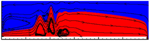
CFD results presented in figure 11 facilitate additional insights into the flow phenomena at the jump and in the upstream and downstream regions. The figure depicts streamline patterns, phase contours, interface profile and velocity distributions at different sections for typical parallel and opposite flow cases. A close observation of the velocity profiles (where the interface is marked by hollow circles) show that for co-current flow, the maximum liquid streamwise velocity occurs at the interface  $(z = h)$ while for counter-current flow, it is either at the interface or below it
  $(z \le h)$. This arises because co-current gas flow aids the liquid in overcoming viscous shear while counter-current gas flow as well as viscous drag at the conduit floor impede liquid flow in the latter case. Also in co-current flow, the maximum gas velocity occurs either at the interface or above it
  $(h \le z \lt H)$ while it lies at the interface
  $(z = h)$ for the counter-current case.
A close observation of figure 11 further reveals the presence of a recirculation zone in the gas phase near the conduit roof close to the inlet (streamline patterns in figure 11(a) and velocity profile in red dashed-dotted curve in figure 11(a 1)). In the velocity profiles presented in figure 11(a 1), the +ve and −ve gas velocities indicate flow separation i.e. flow reversal at an elevation (z) where the velocity is ‘zero’. While gas phase recirculation is expected in the counter-current case, the same in co-current flow is not anticipated and occurs when the interface velocity is large enough such that its effect is propagated upwards. In order to satisfy continuity across a vertical plane, flow reversal takes place above a particular elevation (z). Presence of flow reversal leads to recirculation flow of the gas, as displayed by closed streamlines in figure 11(a). Figure 12 shows that the recirculating gas flow disappears with further increase in gas velocity.
The streamwise velocity profiles as obtained from SWT and CFD simulations are superimposed in figure 13 for a comparative study. We note with interest the shallow water results, which display flow recirculation by +ve and −ve values of velocity across a vertical plane. This demonstrates that, although the analysis obtains a jump as a discontinuity, it can capture the physics of hydraulic jump under two phase laminar flow with much less computational expense and effort. The close agreement evident from the figure justifies the assumption of parabolic profile for both phases upstream and downstream of the jump in SWT.
6.3. Phase diagram
The influence of gas and liquid flow rates on jump types is summarised as a phase diagram in figure 14. The figure consolidates the influence of phase flow rates as obtained from theory. In the field of multiphase flow, phase diagrams are 2-D plots usually drawn with a superficial gas and liquid velocity as the coordinates. Accordingly, figure 14 demarcates the zones of existence for different jump types as a function of gas and liquid flow rates. In the figure, vertical dashed line AB corresponds to zero gas flow rate (i.e. stagnant air above a flowing liquid layer) and the regions to the right and left of AB denote co- and counter-current flow, respectively.
We observe that wavy jumps are favoured by counter-current flow and high liquid flow rate and the transition from a wavy to smooth jump occurs at a lower gas flow rate for higher liquid flows. Submerged jump occurs at low liquid flow rates and is favoured by counter-current flow.
7. Conclusion
We explore a new flow phenomenon – an internal, natural hydraulic jump in plane Poiseuille two-layer flow. The combined analytical, numerical and experimental study presents a comprehensive understanding of the flow singularity and also demonstrates the success of the approximate SWT in analysing a hydraulic jump under two phase flow conditions. SWT not only provides a satisfactory prediction of jump parameters but is also capable of capturing the gas phase recirculation region and jump type for shear induced thin film planar jump for both co- and counter-current gas–liquid flow. In addition, the analysis under limiting flow conditions reduces to the expression for single phase thin film flow.
The following can be concluded from the present investigation:
(i) Counter-current flow favours the formation of wavy jumps and higher phase flow rates are conducive to the formation of a smooth jump.
(ii) Submerged jump is favoured at low velocities and counter-current flow.
(iii) Recirculation region in the gas phase is noted not only for counter-current but also for co-current laminar two phase flow at low gas velocity.
(iv) Both theory and simulation suggest that a substantial increase of co-current gas flow can suppress but not eliminate a viscous shear induced planar jump.
(v) Similar to single phase flow results, the jump location exhibits a nearly linear scaling relationship with liquid flow rate raised to an index of 5/3 at constant gas rate, irrespective of the flow direction.
The present endeavour also suggests that SWT with suitable modifications can be extended to thin film planar jumps in liquid–liquid stratified flow.
Declaration of interests
The authors report no conflict of interest.


