1. Introduction
A causal link between emerging or submerging intracontinental palaeosurface regions with the vertical component of mantle convection has been proposed (Gurnis, Reference Gurnis1990; Burgess & Gurnis, Reference Gurnis1990; Şengör, Reference Şengör, Ernst and Buchan2001b; Heine et al. Reference Heine, Müller, Steinberger and Torsvik2008; Miall, Reference Miall2016). Many of the emerging regions also experienced flood-basalt volcanism, emplacement of giant radiating dyke swarms, radial erosion patterns and continental narrow rifting, followed by broad rifting or continental break-up, leaving numerous signals in the geological record (e.g. Cox, Reference Cox1989; Condie, Reference Condie2001; Şengör, Reference Şengör, Ernst and Buchan2001b; Ernst & Buchan, Reference Ernst and Buchan2001; Rainbird & Ernst, Reference Rainbird, Ernst, Ernst and Buchan2001; Burke & Gunnel, Reference Burke and Gunnel2008; Friedrich et al. Reference Friedrich, Bunge, Rieger, Colli, Ghelichkhan and Nerlich2018; DiCaprio et al. Reference DiCaprio, Gurnis, Müller and Tan2011). Most of these features are well documented and local or regional-scale models have been proposed to explain their formation. However, linking these geological observables to these global physical models of the long-wavelength, low-amplitude vertical motion of the Earth's surface (Steinberger & O'Connell, Reference Steinberger and O'Connell1997; Bunge et al. Reference Bunge, Richards, Lithgow-Bertelloni, Baumgardner, Grand and Romanowicz1998; Bunge, Hagelberg & Travis, Reference Bunge, Hagelberg and Travis2003; Ismail-Zadeh et al. Reference Ismail-Zadeh, Schubert, Tsepelev and Korotkii2004) is hampered by a lack of internally consistent compilation of geological observations at equally long wavelengths (i.e. thousands of kilometres). The gap between the physical models of the plume-mode of mantle convection and the numerous geological features can be closed by applying a unifying stratigraphic framework which translates the plume mode to the geological, geomorphological and stratigraphic records (Friedrich et al. Reference Friedrich, Bunge, Rieger, Colli, Ghelichkhan and Nerlich2018). This framework expresses distinct spatial and temporal relationships of the geological features listed above but requires an internally consistent reference frame to map them. The only reference frames available for such a purpose are interregional-scale or continent-scale geological maps, such as the International Geological Map of the World at 1:35 Million (Bouysse, Reference Bouysse2014), Commission of the Geological Map of the World (CGMW), or the 1:5 Million International Geological Map of Europe and Adjacent Areas (IGME; Asch, Reference Asch2003, Reference Asch2005; Fig. 1). Such maps have not been prepared with this purpose in mind, however.
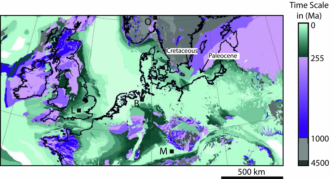
Figure 1. Visualization of hiatus on an exemplary interregional geological map based on the digital version of the 1:5 Million International Geological Map of Europe and Adjacent Regions (Asch, Reference Asch2003, Reference Asch2005). The original map (Asch, Reference Asch2005; Supplementary Fig. S1) has been recoloured as per the legend to emphasize the linearity of geological time across the map. Missing geological time (hiatus) is ubiquitous on this map, based on the missing colour ranges within each set of diverging colours (green, purple and grey). At the resolution of most geological maps, the time represented by hiatus is large; it spans many millions of years (systems) to a few millions of years (series). Higher time resolution (stages, spanning only 1–2 Ma of time) is available and typically compiled on chronostratigraphic charts. Given that landscapes change on scales of 1–2 Ma, hiatus maps at stage resolution would be ideal to capture palaeotopography at any given stage. Interregional geological maps serve as reference frames to document the vertical motion of the Earth's surface. B – Bremen; M – München; L –London; O – Oslo.
The purpose of this paper is to (1) present a simple technique to visualize and quantify long-wavelength vertical motion records by extracting quantitative information in the form of hiatus surfaces from geological maps; and (2) to explore their suitability of serving as an interregional reference frame for vertical surface motion and palaeotopography.
2. Materials and methods
2.a. Interregional unconformities and hiatal surfaces
Geodynamic, tectonic, isostatic, climatic and eustatic processes contribute to the formation of interregional-scale hiatal surfaces. In this way, uplifting surfaces erode over time until the process stops or reverts (inversion) and the region undergoes sedimentary deposition (e.g. Mazur, Scheck-Wenderoth & Krzywiec, Reference Mazur, Scheck-Wenderoth and Krzywiec2005; von Eynatten et al. Reference von Eynatten, Voigt, Meier, Franzke and Gaupp2008). The resulting discontinuity surfaces in the geological record are known as unconformities, preserving time missing (hiatus) from the geological record (e.g. Wheeler, Reference Wheeler1964; Blackwelder, Reference Blackwelder1909; Miall, Reference Miall2010, Reference Miall2016; Prothero & Schwab, Reference Prothero and Schwab2014). Hiatus surfaces are not limited to plate boundary systems, but also occur across continental interiors (Blackwelder, Reference Blackwelder1909; Levorsen, Reference Levorsen1933; Sloss, Krumbein & Dapples, Reference Sloss, Krumbein, Dapples, Longwell, Moore, McKee, Müller, Spieker, Wood, Sloss, Krumbein and Dapples1949; Burgess & Gurnis, Reference Burgess and Gurnis1995; Miall, Reference Miall2016). Such unconformable successions also are widespread at the time resolution of series as shown, for example, on the 1:5 Million International Geological Map of Europe and Adjacent Areas (Asch, Reference Asch2003, Reference Asch2005; Fig. 1).
The existence of such interregional unconformities has been well known for a long time (e.g. Suess, Reference Suess1883; Blackwelder, Reference Blackwelder1909; Stille, Reference Stille1924; Levorsen, Reference Levorsen1933; Sloss, Krumbein & Dapples, Reference Sloss, Krumbein, Dapples, Longwell, Moore, McKee, Müller, Spieker, Wood, Sloss, Krumbein and Dapples1949; Beloussov, Reference Beloussov1962; Sloss, Reference Sloss1963, Reference Sloss1992; Vail, Mitchum & Thompson, Reference Vail, Mitchum, Thompson and Payton1977; Şengör, Reference Şengör2001a, b, Reference Şengör2003; Miall, Reference Miall2010, Reference Miall2016), but few pointed out that physical process-based models are needed to interpret them in their geological context (e.g. Suess, Reference Suess1883; Stille, Reference Stille1924; Burgess & Gurnis, Reference Burgess and Gurnis1995; Şengör, Reference Şengör2016). Recent studies are typically based on quantitative analysis of sedimentary basins (e.g. Japsen et al. Reference Japsen, Chalmers, Green and Bonow2012; Kukla, Strozyk & Mohriak, Reference Kukla, Strozyk and Mohriak2018; Vibe et al. Reference Vibe, Friedrich, Bunge and Clark2018), landscapes (e.g. Green et al. Reference Green, Japsen, Chalmers, Bonow and Duddy2018; Guillocheau et al. Reference Guillocheau, Simon, Baby, Bessin, Robin and Dauteuil2018) or mountainous regions (Prenzel et al. Reference Prenzel, Lisker, Monsees, Balestrieri, Läufer and Spiegel2018; Sehrt et al. Reference Sehrt, Glasmacher, Stockli, Labour and Kluth2018), but need to be assimilated in vertical surface motion models at interregional scales (e.g. Baran, Friedrich & Schlunegger, Reference Baran, Friedrich and Schlunegger2014).
Numerous protocols exist to visualize interregional unconformities. Stille's (Reference Stille1924) time charts of transgressions and regressions were intended to seek global correlation, but today we understand why truly coeval global records cannot exist on the Earth (e.g. Sloss, Krumbein & Dapples, Reference Sloss, Krumbein, Dapples, Longwell, Moore, McKee, Müller, Spieker, Wood, Sloss, Krumbein and Dapples1949; Pitman & Golovchenko, Reference Pitman, Golovchenko, Müller, McKenzie and Weissert1991; Church et al. Reference Church, White, Coleman, Lambeck and Mitrovica2004; Şengör, Reference Şengör2016; Friedrich et al. Reference Friedrich, Bunge, Rieger, Colli, Ghelichkhan and Nerlich2018). Sloss, Krumbein & Dapples (Reference Sloss, Krumbein, Dapples, Longwell, Moore, McKee, Müller, Spieker, Wood, Sloss, Krumbein and Dapples1949) point out that sedimentary sequences are bounded by regional unconformities that are not coeval; neither globally coeval stratigraphy nor globally coeval episodicity in orogeny exists (Şengör, Reference Şengör2016). Wheeler (Reference Wheeler1958) constructed time–distance diagrams to visualize gaps in the sedimentary record. Sloss (Reference Sloss1963) defined stratigraphic sequences as ‘rock-stratigraphic units traceable over major areas of a continent and bounded by unconformities of interregional scope’.
2.b. Extracting palaeotopographic information from geological maps
Mapping the full extent of unconformities in time and space is a prerequisite for understanding their significance in the geological record (e.g. Sloss, Krumbein & Dapples, Reference Sloss, Krumbein, Dapples, Longwell, Moore, McKee, Müller, Spieker, Wood, Sloss, Krumbein and Dapples1949; Beloussov, Reference Beloussov1962; Sloss, Reference Sloss1963). Interregional-scale geological maps display unconformity- and succession-boundary surfaces as linear traces (Fig. 1). The distribution of geological formations at a particular datum in the past is shown as palaeogeological maps. Levorsen (Reference Levorsen1933) constructed such maps for the base datum of three series across North America, confirmed agreement between the mapped pattern and independently compiled structural information, and concluded that such maps – in conjunction with isopach maps – yield palaeotopographic highs and lows. Because comparison against physical models requires quantification of geological data, we go one step further here by plotting hiatus area as a quantifiable proxy for palaeotopography to visualize and explore dimensions, shapes, ages and duration of hiatus surfaces in millions of years.
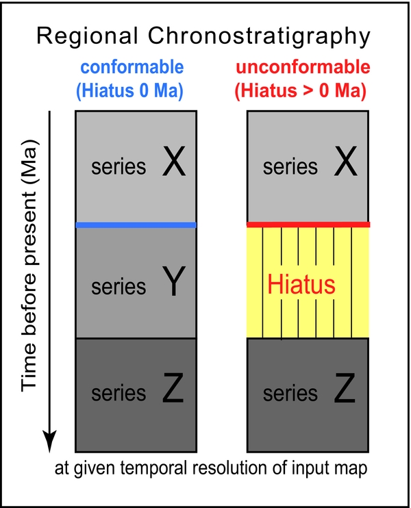
The lower boundary of a key or datum horizon (cf. Levorsen, Reference Levorsen1933) is either conformable or unconformable at the given temporal resolution (Fig. 2). For conformable contact surfaces, the hiatus duration is equivalent to zero at the resolution of the mapped units (e.g. systems, series or stages). Its nominal uncertainty is by definition zero. However, this does not imply that a succession is truly conformable in nature; rather, it simply means that it is conformable at the mapped temporal resolution (Fig. 3a, b). For unconformable contact surfaces, the hiatus duration (in millions of years, Ma) is equivalent to the geological duration of system(s), series or stage(s) that are missing below the datum horizon of a system, series or stage (Fig. 2). The temporal resolution of the geological map provides an uncertainty in hiatus duration that spans up to the duration of the next older and the next younger system, series or stage (Fig. 3c, d).

Figure 2. Schematic regional chronostratigraphic columns defining conformable (blue) and unconformable (red) succession boundaries as used in this study. Hiatus is defined as the missing geological record. The hiatus duration is defined by the upper and lower boundary of the missing series Y. For the purposes of this paper, there is no distinction made between degradational vacuity (erosion) and hiatus formed by non-deposition (Wheeler, Reference Wheeler1964); both are referred to as hiatus.

Figure 3. Diagrammatic chronostratigraphic sections to illustrate hiatus uncertainties and how hiatus duration (intensity) is calculated for conformable and unconformable boundaries. Input maps for (a) a conformable chronostratigraphic section and (c) an unconformable section. Real data for (b) a conformable chronostratigraphic section and (d) an unconformable section, in which a and b refer to the ages of the upper and lower boundary of the series, respectively. To obtain positive hiatus values, the age of the younger series (X) is subtracted from the age of the older series (Z). Despite apparent zero hiatus (XYZ) at the temporal resolution of series, in reality a hiatus of duration (Yb – Xa) may be hidden in the data (Equation (b)). Geological input data at the resolution of stages (b) will reveal and minimize this problem, but such digital maps do not yet exist at interregional scales.
2.c. Construction of hiatus surface contour maps
Hiatus surface area and contour maps can be produced for the base of the datum horizon of each succession shown on a geological map, and for the present day. Figure 4 illustrates the method on interregional scales, assuming a temporal resolution of series, but this concept applies equally to systems or stages. Consider the basal contact of series X, that is, the time represented by the boundary between series Y and series X (Figs 2, 3a, 4a). The uncertainty associated with this time is 0 Ma (Figs 2, 3a), but it is larger in reality depending on the age of successions exposed locally (Fig. 3). This boundary marks the idealized temporal reference frame of interest on a given geological map (Fig. 4c) to construct a hiatus surface and contour plot (Fig. 4d). The basal contact of series X on Figure 4c is mapped as either conformable (blue, colour online) or unconformable (red), depending on which succession directly underlies series X on the map.

Figure 4. Internally consistent schematic diagrams and maps displaying hiatus area information in time and space at the temporal resolution of geological series. (a) Interregional chronostratigraphic section showing the full temporal extent of hiatus duration. (b) Hiatus values are assigned to the conformable and unconformable boundaries based on missing series. Small circles filled in white (outer) represent anchor points between conformable and unconformable boundary segments and define the termination of a hiatus area. Small circles filled in black (inner) mark an increase in hiatus value. (c) Geological map derived from the information on the chronostratigraphic charts shown in (a) and (b). (d) Hiatus area map derived from the geological map constituting a proxy for palaeotopography. Blue represents the region where the base of series X rests conformably on older series, representing topographically lower regions; red highlights regions of hiatus area at the base of series X, representing topographically higher regions.
For example, in the centre of Figure 4c, basement is exposed adjacent to series X such that the hiatus along this contact segment is equivalent to the time represented by missing series Y and Z (Fig. 4a, b). Adjacent to the basement region, the basal contact of series X is exposed adjacent to series Z, corresponding to a hiatus duration equivalent to series Y. No hiatus (0 Ma) occurs on both the left- and right-hand side of the central region and is defined by continuity in successions Z, Y and X. Regions where series X successions are exposed mark regions of deposition and cover hiatus information in the subsurface (Fig. 4c). In such regions, additional data need to be integrated such that the width dimension of the hiatus surface, which arguably continues below series X, can be defined.
Of greatest importance in constructing the hiatus surface maps are the lateral termination lines that mark transitions from conformable to unconformable contact areas along the datum horizon (here series X). On Figure 4d, these are marked as white filled circles (anchor points). The distance between these anchor points defines the length dimension of the hiatal surface area within the spatiotemporal reference frame; along this direction, it relates to the maximum permissible wavelength of the causal process(es). The width of the hiatus area is not constrained on the conceptual map in Figure 4c, but in reality additional anchor points may be found on the map or may be inferred from subsurface data, thereby defining the maximally permissible shape of a hiatal area.
A plot of iso-hiatus duration in Ma (as defined by the temporal resolution of the mapped successions) is constructed by mapping areas of equal hiatus values (Fig. 4d). Hiatus area maps are opposite in sign and scope from isopach maps of sedimentary successions because hiatus surfaces represent the missing section, not the sedimentary record. The map is coloured in blue (colour online) where the basal contact of series X is conformable (hiatus value = 0), and in red where the hiatus value corresponds to series Y or series Y + Z in this example. The region marked in red is therefore the hiatus surface area that was affected by any combination of erosion and non-deposition, which on interregional scales is assumed to correspond to the vertical uplift of Earth's surface. Figure 4d shows one permissible hiatus surface area map consistent with the anchor points and distribution of conformable versus unconformable datum segments. At a higher temporal resolution of mapped successions for the same region, different patterns of hiatus surface intensity emerge, implying that this hiatus surface pattern is highly dependent upon scale.
Subtraction of an older hiatus datum surface from a younger one reveals temporal changes in the spatial hiatus pattern between two key datums (e.g. Fig. 5c). Such figures show areas that change from conformable to unconformable or vice versa. This step also serves to subtract hiatus from the datum surfaces that formed prior to the key datum of interest.
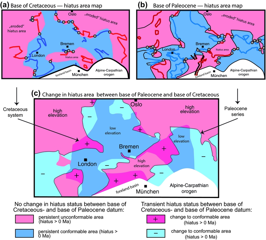
Figure 5. Palaeogeological hiatus area maps for (a) the base Cretaceous and (b) the base Paleocene datum and (c) their change over time based on the IGME 5000 of Asch (Reference Asch2003, Reference Asch2005). Construction of the maps is based on the procedure shown in Supplementary Figures S1 and S2. Thick black lines mark the trace of the younger Rhine Graben system that affected the hiatus areas only locally. The white region marks the alpine orogenic system and its foreland where plate boundary effects related to the plate mode dominate. (c) Differential hiatus map showing the superposition of the hiatus areas in (a) and (b) above. Black arrows point to the shape of the hiatus regions for the base Cretaceous and the base Paleocene, respectively, as shown in (a) and (b). A change from conformable to unconformable boundary is represented by dark red colours and a ‘+’ symbol, representing uplift. A change from unconformable to conformable boundary is represented by light blue colours and a ‘–’ symbol, representing topographically low regions and sediment accumulation across the time boundary at the mapped resolution. In general, regions in red colours are interpreted as having undergone steady or transient uplift and those in blue as having undergone steady or transient subsidence relative to their surroundings.
3. Example based on the 1:5 million IGME
3.a. Construction of palaeogeological hiatus maps
A portion of the IGME 5000 (Asch, Reference Asch2003, Reference Asch2005; Fig. 1) is used to illustrate the hiatus mapping method, and the base of the Cretaceous system is used as an exemplary datum (Supplementary Fig. S1a, b, available online at http://journals.cambridge.org/geo). Contact segments are marked as either conformable (blue) or unconformable (red) as shown in Figures 2 and 4 (cf. Supplementary Figs S1, S2). A hiatus duration in millions of years is assigned to each basal segment based on the difference in age between the datum and the age of the adjacent system or series (Fig. 4b). Assuming that, at a specific time interval and spatial scale, any landscape is in either erosion- or sediment-deposition-mode, the hiatus surface can be mapped (Supplementary Fig. S1b, c) and contoured (Fig. 6a; Supplementary Fig. S3a).
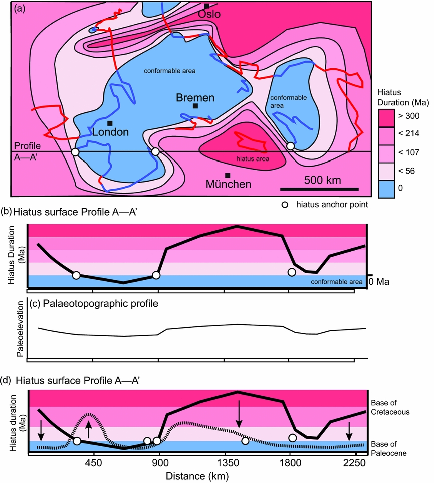
Figure 6. (a) Structural contour map showing the hiatus surface for the base of the Cretaceous system for central Europe and surroundings based on the digital version of the IGME 5000 (Asch, Reference Asch2005), with (b) hiatus profile revealing long-wavelength variations in hiatus duration, and (c) conversion to palaeotopography in a conceptual way. A quantitative conversion requires integration with other geological data, in particular those that yield rates of exhumation. (d) As for (b) but with curve for the base Paleocene. The arrows indicate the direction of change between the base of the Cretaceous datum and the base of the Paleocene datum. See also Supplementary Figure S3 for the construction of the base Paleocene curve.
The anchor points are marked at the transition from conformable to unconformable along the basal datum (Fig. 4b, c; Supplementary Fig. S1c, available online at http://journals.cambridge.org/geo). Major plate-boundary signals such as the Alpine–Carpathian orogen are excluded, and smaller, high-frequency signals such as those produced by the Rhine graben have only local significance. The procedure is then repeated for the key datum at the base of the Paleocene (Supplementary Fig. S2); profile A–A’ for both the base of the Cretaceous and the base of the Eocene are plotted in Figure 6d. Finally, the difference in hiatus surface area between the base of the Cretaceous (Fig. 5a) and the base of the Paleocene (Fig. 5b) is derived by subtracting the older from the younger hiatus areas (Fig. 5c). Figure 5c serves to visualize the size of the area that changed from being conformable to non-conformable and vice versa. Regions that changed from conformable to unconformable are marked in pink and with a plus sign (transient uplift), whereas those regions that changed from being unconformable at the base of the Cretaceous to being conformable at the Paleocene datum are marked in light blue with a minus sign (transient subsidence).
3.b. Results
The hiatus area maps illustrate spatial variations in time missing from the rock record based on the geological input map (here, IGME 5000; Asch, Reference Asch2003, Reference Asch2005). Both hiatal surface maps (Fig. 5a, b) yield large coherent conformable and non-conformable areas, but of different shape, location and dimension. The long dimension of a hiatus area for the basal Cretaceous datum is at c. 1000 km in an E–W-aligned direction, but its N–S direction is truncated by the alpine front (Fig. 5a, b). Two conformable surface areas of c. 1000×500 km and 800×200 km dominate the map and indicate that sedimentary deposition at the resolution of series was continuous across the Jurassic–Cretaceous system boundary at the resolution mapped on the IGME 5000 (Asch, Reference Asch2005). At the base of the Paleocene datum, a well-defined hiatus surface of >1000 km in dimension is oriented SW–NE and perhaps connects to the large hiatus area in NE Europe (Scandinavia and surrounding regions; Supplementary Fig. S2, available online at http://journals.cambridge.org/geo). Another large hiatus area occurs in a N–S direction between Ireland and England. The shape of the conformable area is elongated in a SW–NE direction between London and Bremen, but changes to a NNW-aligned direction following the long axis of the North Sea graben system.
The erosional area north of Munich persisted since prior to Cretaceous time but, based on the data shown on the IGME 5000 (Asch, Reference Asch2003), it decreased in intensity (Fig. 6d), changed its shape and doubled in size (Fig. 5c) compared with the base of the Paleocene datum. The direct comparison between the hiatal and depositional surfaces at the respective bases of the Cretaceous and the Paleocene reveals that about half of the region shown on the map underwent a transition from hiatus to conformity or vice versa (Fig. 5c). New hiatus areas (marked with a plus sign in Fig. 5c) formed SW and north of London as well as NW of Munich and to the east of Bremen, whereas over the same time interval a net surface area two times larger experienced a change to conformable boundaries (marked with a minus sign in Fig. 5c), yielding net subsidence of the region by the beginning of Paleocene time.
4. Meaning of the hiatal surface areas
To first order, the presence of hiatus areas below a geological base datum define the dimensions, shapes and duration of regions undergoing long-lasting and broad erosion and/or non-deposition, which at the scales invoked is a proxy for a combination of exhumation and surface uplift (cf. England & Molnar, Reference England and Molnar1990). The duration over which the hiatus area is defined relates to the magnitude of the underlying processes, but it depends strongly on the time resolution of the input geological map. Temporal changes in hiatus surface duration, which are obtained by subtracting the respective older from the younger surfaces, yield the evolution of palaeotopography averaged over large time and space scales (e.g. Fig. 5c).
On interregional scales, these palaeo-landscapes formed through a combination of plate-boundary processes and long-wavelength vertical motion of the Earth's mantle (dynamic topography). Shallow-marine regions and coastal plains are also sensitive to eustatic sea-level variations. The character and rate of source-to-sink sediment production, transport and deposition is additionally modulated by climatic effects. The sum of changes in vertical position of the Earth's surface caused by the abovementioned processes is further affected by isostatic adjustments to loading and unloading of the crust. The net elevation of any point on the Earth's surface is therefore determined by the integral of all physical and chemical processes acting on this point. Knowledge of the timing, magnitude and spatial dimension of the underlying processes will therefore guide any interpretation of the hiatus area maps (e.g. Friedrich et al. Reference Friedrich, Bunge, Rieger, Colli, Ghelichkhan and Nerlich2018; Vibe et al. Reference Vibe, Friedrich, Bunge and Clark2018).
By calibrating hiatus duration using independent geological data (kilometres per million years, km Ma–1) in context with physical models that supply the spatial and temporal boundaries, the hiatus surface maps (in millions of years) can be turned into quantitative maps of palaeotopography (in kilometre) across interregional scales. Hiatus areas and their changes over time are therefore proxies for palaeotopography and indicators of change in palaeo-elevation and vertical motion of the Earth's surface.
5. Discussion
5.a. Uncertainties and limitations in constructing hiatus surfaces
Hiatus surface maps are well constrained in dimension but not in amplitude, because this requires calibration using independent geological data such as thermochronological data. The true hiatus is likely longer than indicated by the missing system(s) or series because, at any one location, sedimentary successions represent only a small portion of a system or series (Fig. 3). For example, temporal uncertainties of up to nearly 100% may be encountered on currently available digital geological maps, even in cases where only one system or series is absent and the adjacent systems or series are not fully represented in the field (Fig. 3). Interregional geological maps at the resolution of stages (1–2 Ma) will reduce these uncertainties by displaying the true age and duration of deposition of a geological unit more precisely. In contrast, improved direct dating of stage boundaries through a combination of biostratigraphic and radiometric techniques and higher sampling density across hiatus surfaces reduces hiatus duration.
The spatial dimension of the hiatus surface duration (its wavelength) is also dependent upon scale. The true dimensions of the hiatus surface are not visible at series resolution; stages are required. Such information exists as chronostratigraphic charts (e.g. Menning & Hendrich, Reference Menning and Hendrich2002; Hopper et al. Reference Hopper, Funck, Stoker, Arting, Peron-Pinvidic, Doornenbal and Gaina2014), which include compilations of stratigraphic relationships for adjacent regions. Within the interregional hiatus mapping approach described here, the regional sections can be placed on laterally coherent maps by using the anchor point concept described above.
Some or all of a hiatus surface area may have formed at an earlier time. Older hiatus surfaces must therefore be subtracted from younger ones, which may introduce large uncertainties in the hiatus contouring. Calibration of hiatus area by assimilating independent geological data will minimize this problem. Hiatus areas may merge laterally with adjacent hiatus areas. Empirical determination of the underlying causes is therefore impossible. Process-based models that have clear initiation times and initiation centres must be invoked (e.g. Sengör, Reference Şengör2016; Friedrich et al. Reference Friedrich, Bunge, Rieger, Colli, Ghelichkhan and Nerlich2018).
The hiatus method has no resolving power in regions that experienced general conformable contact relationships, which correspond to depositional regions and hence regions that subside or remain at lower-than-average elevations than surrounding regions. Integration of geological data from basins with those from adjacent landscapes is required to complement mapping of the time-based surfaces.
A further bias in the compilation, visualization and interpretation of detailed geological data is that they most often are best preserved, resolved and accessible at the margins of uplifting or subsiding regions. There, even small changes in vertical motion of the Earth's surface lead to changing depositional environments, including a switch from deposition to erosion and vice versa. Because these marginal regions are generally sensitive recorders of all dynamic, tectonic, isostatic and climatic processes, the detangling of these effects is difficult and has resulted in the development of techniques to determine the underlying processes empirically (e.g. Vail, Mitchum & Thompson, Reference Vail, Mitchum, Thompson and Payton1977; Vail, Hardenbol & Todd, Reference Vail, Hardenbol, Todd and Schlee1984; Haq, Hardenbol & Vail, Reference Haq, Hardenbol and Vail1987; Geel, Reference Geel2000). Numerous studies have since then highlighted the limited value of empirical stratigraphy (e.g. Summerhayes, Reference Summerhayes1986; Christie-Blick, Mountain & Miller, Reference Christie-Blick, Mountain and Miller1990; Miall, Reference Miall1991; Şengör, Reference Şengör2016).
However, the maximum magnitude of the vertical-motion signal typically occurs far from the margins in the centres of uplifting or subsiding regions. This provides an opportunity to map the entire signals of vertical motion from centres to their margins, that is, from where the signal is largest to where it is within the noise. Data collection near the terminations of basins or mountains where (by definition) the signals converge to zero is therefore difficult, but required to build physically based observational models of the palaeotopographic evolution of the Earth's surface. The identification of large hiatus surfaces of geodynamic origin (epeirogeny in the sense of Stille, Reference Stille1919, Reference Stille1924) is hampered in particular by traditional geological studies of local records that are not known or mapped in their full dimensions and shape.
5.b. Palaeogeological hiatus maps versus chronostratigraphic charts and palaeogeographic maps
Because local geological records are rich in information, they have been compiled preferably as chronostratigraphic charts (e.g. Ziegler, Reference Ziegler1990, stratigraphic correlation charts, enclosures 44–52; Scotese & Golonka, Reference Scotese and Golonka1997; Evans, Reference Evans2003; Burke & Gunnell, Reference Burke and Gunnel2008; Doornenbal & Stevenson, Reference Doornenbal and Stevenson2010; Green et al. Reference Green, Lidmar-Bergström, Japsen, Bonow and Chalmers2013; Hopper et al. Reference Hopper, Funck, Stoker, Arting, Peron-Pinvidic, Doornenbal and Gaina2014; Kemnitz et al. Reference Kemnitz, Ehling, Elicki, Franzke, Geyer, Linnemann, Leonhardt, Plessen, Rötzler, Rohrmüller, Romer, Tichomirova and Zedler2017, figs 1, 2; Torsvik & Cocks, Reference Torsvik and Cocks2017). The temporal resolution of the charts is excellent, that is, on the same scale as the rates at which geodynamic and climatic processes occur (1–2 Ma or geological stages), but the spatial information is truncated by vertical lines to maximize the number of columns that fit on such charts side by side (e.g. Ziegler, Reference Ziegler1990, enclosures 44–52); true lateral interfingering of contact relationships is therefore sacrificed on such charts. Palaeogeological hiatus maps are well suited to visualize information compiled on chronostratigraphic charts in their true spatial dimension.
Another significant difference between palaeogeological hiatus area maps and palaeogeographic maps is that the latter focus on the wealth of data from sedimentary basins (Ziegler, Reference Ziegler1990; Scotese & Golonka, Reference Scotese and Golonka1997; Evans, Reference Evans2003; Burke & Gunnell, Reference Burke and Gunnel2008; Doornenbal & Stevenson, Reference Doornenbal and Stevenson2010; Hopper et al. Reference Hopper, Funck, Stoker, Arting, Peron-Pinvidic, Doornenbal and Gaina2014; Torsvik & Cocks, Reference Torsvik and Cocks2017), whereas the former focus on data from eroding regions. Principally, chronostratigraphic reference charts which form the basis for palaeogeological and palaeoenvironmental maps contain detailed records of hiatus, but the accompanying palaeogeographic maps only show the distribution of sedimentary facies and depositional environments (e.g. Ziegler, Reference Ziegler1990, enclosure 28 for the Jurassic–Cretaceous boundary), whereas regions of non-deposition are shown in uniform grey shades. Information about vertical motion is indicated on the correlation charts, marking hiatus, but their geometry and dimensions cannot be inferred from them. However, based on recent progress in understanding the plate- and the plume mode of mantle convection, a need has arisen to place all of the information available on traditional maps and charts (such as unconformities, fault systems, uplift, volcanic rocks, erosional hiatus versus non-depositional hiatus) back on appropriate maps (Ernst & Buchan, Reference Ernst and Buchan2001; Sengör, Reference Şengör2016; Friedrich et al. Reference Friedrich, Bunge, Rieger, Colli, Ghelichkhan and Nerlich2018). The anchor-point technique described above may serve to define the dimensions contained within chronostratigraphic charts.
5.c. Potential applications and future perspectives
The hiatus visualization tool may be applied to a wide range of problems and data. For example, compilation of a sequential global hiatus map at the temporal resolution of systems and series, plotted in the reference frame of Matthews et al. (Reference Matthews, Maloney, Zahirovic, Williams, Seton and Müller2016) using G-Plates (Boyden et al. Reference Boyden, Müller, Gurnis, Torsvik, Clark, Turner, Ivey-Law, Watson, Cannon and Keller2011; see fig. 5 in Friedrich et al. Reference Friedrich, Bunge, Rieger, Colli, Ghelichkhan and Nerlich2018), reveals transient long-wavelength signals across most continents since the break-up of Pangaea. In particular, the age and duration of hiatus surfaces within Africa and the Americas appears to be broadly coeval to the opening of the South Atlantic Ocean (e.g. Burke & Gunnel, Reference Burke and Gunnel2008; Colli et al. Reference Colli, Stotz, Bunge, Smethurst, Clark, Iaffaldano, Tassara, Guillocheau and Bianchi2014; Barnett-Moore et al. Reference Barnett-Moore, Hassan, Müller, Williams and Flament2017; R. Neofitu, unpub. MSc thesis, Ludwig-Maximilians-University of Munich, 2017; Bunge & Glasmacher, Reference Bunge and Glasmacher2018; Neofitu & Friedrich, Reference Neofitu and Friedrich2018). Although geodynamic models of global mantle convection predict such regions of dynamic topography in context with the plume-mode of mantle convection (e.g. Hager et al. Reference Hager, Clayton, Richards, Comer and Dziewonski1985; Davies, Reference Davies1999), rigorous testing of these models has not yet succeeded except on local and regional scales that document episodic uplift (e.g. Japsen et al. Reference Japsen, Chalmers, Green and Bonow2012; Green et al. Reference Green, Lidmar-Bergström, Japsen, Bonow and Chalmers2013, Reference Green, Japsen, Chalmers, Bonow and Duddy2018; Guillocheau et al. Reference Guillocheau, Simon, Baby, Bessin, Robin and Dauteuil2018). However, these spatial and temporal patterns are so complex that consensus over the direct causes has not yet been reached (for a summary see Bunge & Glasmacher, Reference Bunge and Glasmacher2018). A physical framework to tie the geodynamic predictions to the geological record is needed before such models can be tested rigorously. As a direct result of the sequential visualization of hiatus surfaces on the continent-scale, Friedrich et al. (Reference Friedrich, Bunge, Rieger, Colli, Ghelichkhan and Nerlich2018) developed a unified plume-stratigraphic framework and translated the effects of a rising mantle plume into dynamic topography and a detailed stratigraphic record; several hiatus surface areas are predicted to form solely due to a rising plume accompanied by dome uplift, erosion, inversion of the plume margin, and distal sedimentation (cf. Friedrich et al. Reference Friedrich, Bunge, Rieger, Colli, Ghelichkhan and Nerlich2018, figs 8, 9). At this scale, the hiatus maps derived from geological data may be useful for direct comparison with dynamic topography predicted by geodynamic models of mantle convection (e.g. Colli, Ghelichkhan & Bunge, Reference Colli, Ghelichkhan and Bunge2016; Bunge & Glasmacher, Reference Bunge and Glasmacher2018; Friedrich et al. Reference Friedrich, Bunge, Rieger, Colli, Ghelichkhan and Nerlich2018; Neofitu & Friedrich, Reference Neofitu and Friedrich2018).
Hiatus mapping may also be applied to subsurface data. Yildirim & Friedrich (Reference Yildirim and Friedrich2018) developed sequential hiatus surface areas for Palaeogene and Neogene series within the Northern Alpine foreland basin by extracting hiatus information from detailed geological maps, well logs and published stratigraphic sections. In seeking to compile chronostratigraphic data, it became clear that many sections contain lithostratigraphic facies information that may have been dated in one distant location, but not everywhere across the basin (E. Yildirim, unpub. MSc thesis, Ludwig-Maximilians-University of Munich, 2016). Because of the potential of temporal migration of lithofacies across a basin, it is impossible to assign age information to such units by techniques that rely on spatial correlation, such as tracing of seismic reflectors or gamma-ray logs (cf. Christie-Blick, Mountain & Miller, Reference Christie-Blick, Mountain and Miller1990; Miall, Reference Miall2010; Şengör, Reference Şengör2016). Such sections must be dated directly using biostratigraphic or radiometric methods. As in the interregional example discussed above, the hiatus method is very sensitive to temporal resolution; it is therefore currently hampered by a lack of such information.
Tectonic and climatic processes operate on overlapping scales, typically on the order of millimetres per year, metres per thousand years or kilometres per million years. Rates of horizontal and vertical motion of the Earth's surface through the plate mode, the plume mode and isostatic responses of the crust are also expected to range from millimetres to up to tens of centimetres per year (e.g. Davies, Reference Davies1999; Friedrich et al. Reference Friedrich, Wernicke, Niemi, Bennett and Davis2003; Kreemer, Holt & Haines, Reference Kreemer, Holt and Haines2003; Argus, Gordon & DeMets, Reference Argus, Gordon and DeMets2011; Colli, Ghelichkhan & Bunge, Reference Colli, Ghelichkhan and Bunge2016). In order to understand the effects of either mode, palaeotopographic reconstructions at a temporal resolution of 1–2 Ma (i.e. one to two stages) is needed to determine age and duration of hiatus surfaces at the rate of these natural processes. This information is generated based on a combination of radiometric age determination with biostratigraphic analysis of well logs and outcrop mapping (e.g. Gradstein et al. Reference Gradstein, Ogg, Schmitz and Ogg2012).
In order to visualize any vertical motion records at long wavelengths (a few thousands of kilometres) and low amplitude (1 to <3 km), geological maps need to be compiled at the scale of the continents and with the temporal resolution of stages. This can be accomplished by either using existing maps at scales of, for example, 1:200000, which currently contain a temporal resolution of stages, and connecting them on continent scales. Alternatively, a next generation of maps at intercontinental scales of, for example, 1:5 million need to be synthesized from detailed information. Ideally, hiatus surface mapping is achieved on a global scale by filling in regional information. This strategy is preferred over synthesizing information on detailed local or regional maps; the large amount of information on such maps is likely to contain data on a range of scales. Geological data can be added systematically to convert hiatus patterns into palaeotopography.
6. Conclusions
There is a need to interpret hiatus maps in conjunction with physical models of the vertical Earth surface motion, such as global mantle convection models. The construction of hiatus surfaces allows the visualization of the dimension, shape, pattern, age and duration of missing time in the geological record by applying a single manipulation to existing interregional-scale geological maps. The hiatus surface maps are laterally coherent beyond the dimension of individual sedimentary basins and mountains. It is necessary to compile geological maps at interregional scales and at the temporal resolution of stages, most of which span 1–2 Ma in duration, because the Earth's vertical surface motion changes on time scales of a few millions of years. Calibrated against other geological data, hiatus information may be quantified from which the relative vertical surface motion, hence the palaeotopography, can be derived. The palaeogeological hiatus maps must be corrected for hiatus that formed at local scales or at older time intervals. Future improvements of this technique require interregional-scale geological maps with higher temporal resolution (e.g. stages) to display the full temporal and spatial signal at which the Earth's surface moves vertically. The hiatus mapping method is a first-order technique that may be easily applied on any scale and is suitable to map any expression of vertical motion of the Earth's surface, ranging in scale from salt domes to mantle plumes. The wealth of geological data needs to be interpreted with the aid of physical models, not empirically. Geological mapping, radiometric dating and biostratigraphy remain essential tools of choice to identify time horizons of interregional significance.
Acknowledgements
This research received no specific grant from any funding agency, commercial or not-for-profit sectors. I thank Hans-Peter Bunge for asking me whether quantifiable information bearing on vertical surface motion may be extracted from geological maps, which prompted this paper. I also thank Vladimir Shipilin, who modified the colour scheme in the IGME 5000 using ArcGIS, and Kristine Asch, BGR Hannover, for providing the shape file for the IGME 5000 map. Constructive reviews by Christian Heine, Celal Şengör and Guido Meinhold helped to improve the manuscript.
Declaration of interest
None.
Supplementary material
To view supplementary material for this article, please visit https://doi.org/10.1017/S0016756818000560