Introduction
The wireless sensor networks are more and more widely used for different purposes, such as for electromagnetic spectrum monitoring [Reference Akyildiz, Su, Sankarasubramaniam and Cayirci1–Reference Liu, Dousse and Towsley6]. Many algorithms for spectrum sensing have been proposed. The main functionality of sensing algorithms is signal detection that is particularly challenging due to short observation time and low signal-to-noise ratio (SNR) requirements. In real-world applications, the suitability of sensing algorithms must be evaluated considering sensing algorithms practical implementation problems and it is also necessary to consider how sensing functionality can be integrated within the overall network [Reference Haykin7].
This paper presents the issue of deployment optimization of wireless sensors, with a limited area of coverage. To increase the monitored area, it is necessary to make use of a cooperating sensors network, where the monitoring nodes exchange information between each other, in order to achieve a common result. A key element is a global coverage area of all deployed sensors [Reference Huang and Tseng8, Reference Gupta, Kumar and Jain9]. The above issue is also useful for the cognitive radio network, to mitigate potential interferences [Reference Haykin7, Reference Marshall10]. It can increase their situation awareness functionality, and enable the creation of Radio Environment Map (REM) [Reference Yilmaz, Tugcu, Alagoz and Bayhan11]. The proposed criteria and methods enable also minimization of the nodes shadowing or hidden node problem [Reference Fette12], which are especially important in urban areas. In addition, the cooperative sensing gives more precise and realistic picture of the electromagnetic situation. To achieve the mentioned goals, it is necessary to exchange data between nodes which is particularly difficult in the case of wireless communication.
In [Reference Liu, Dousse and Towsley6] authors consider coverage in case of mobile sensor networks. In such cases, areas covered by sensors change over time and depends on the mobility behavior. Paper [Reference Shakkottai, Srikant and Shroff13] presents an unreliable wireless sensor grid-network with nodes placed in a square of unit area, however, authors assumed fixed sensing radius. There are also other papers e.g., [Reference Howard, Mataric and Sukhatme14, Reference Batalin and Sukhatme15] which address the problem of coverage sensor networks in an unknown environment without a priori global information about the interested area assuming that communication between sensors is already established.
Our proposed solution generates optimized sensor network configuration, taking into account digital terrain model, buildings, sensors parameters, and expected coverage redundancy of specified areas.
The previous work of the authors about the use of a wireless sensor network to monitor the spectrum in urban areas can be found in [Reference Malon, Skokowski and Łopatka16]. The other authors’ paper [Reference Skokowski, Malon, Kelner, Dolowski and Lopatka17] concerns the dedicated sensing scheme and implementation to enable adaptive channels selection for cognitive radio networks. Time division multiple access scheme, where dedicated time slots are assigned to sensing whereas others to communications, is proposed.
Problem definition
Let us define M and N variables to denote the number of sensors and the number of potential transmitters, respectively. For the above-mentioned groups of points, the path loss calculations were performed.
The attenuation symmetry between two points was assumed:
 $$pathLoss(m,n) = pathLoss(n,m),$$
where:
• pathLoss(m,n) – path loss between m and n points [dB].
The detection result of a signal received in point m, generated in point n, assuming 0 dBi antenna gains, was defined as:
 $$detRes{\rm (}m{\rm,} \,n{\rm )} = \left\{ {\matrix{ {1,\;{\rm for}\;rxLevel + pathLoss(m,n) \le txLevel,} \cr {0\;{\rm for}\;{\rm others},} \cr}} \right.$$
where:
• rxLevel – received signal level at the sensor input, which enables correct signal detection [dBm],
• txLevel – signal level at the detected transmitter output [dBm].
The detailed link budget analysis can be found in e.g. [Reference Marshall10] and for transceiver design and parameters description please refer to [Reference Bullock18].
Assuming that antenna gains of sensors are the same, and taking into account radio attenuation symmetry between sensors (1), the following relationship is also correct:
 $$detRes(m,n) = detRes(n,m).$$
The coverage of signal detection possibility for a specified area, calculated for a sensor located in point m, was determined as follows:
 $$detCov{\rm (}m) = \displaystyle{{\sum\nolimits_{n = 1}^N {detRes(m,n)}} \over N} \times 100\;[\% ],$$
 $$detCov(m) \in \left\langle {0,100} \right\rangle. $$
If in a given region there is more than one sensor (M > 1), the obtained outcome may be a cooperative detection result for the signal generated in point n:
 $$detResCoop{\rm (}n) = \sum\limits_{m = 1}^M {detRes(m,n)}, $$
 $$detResCoop(n) \in \left\langle {0,M} \right\rangle. $$
Due to the fading effect, reflections and interferences, there is a nonzero probability of missed detection by any individual sensor. This undesirable phenomenon can be minimized by redundancy, which means that the source of the signal should be in the range of more than one sensor, and that can be achieved by appropriate selection of sensors locations. Therefore, the coverage of signal detection possibility for a specified area calculated in all M points (sensors locations), is the cooperative result with the redundancy r and can be written as:
 $$\det CovCoop_r = \displaystyle{{ \vert \{ n \in N:detResCoop(n) \ge r\} \vert} \over N} \times 100\;[\% ],$$
 $$\det CovCoop_r \in \left\langle {0,100} \right\rangle, $$
 $$r \in \left\langle {1,M} \right\rangle. $$
For the particular redundancy r, the importance ratio (weighting factor) w r was proposed. It enables to determine the priority regions of special interest.
Using the above-defined values, the objective function was proposed:
 $$f = \sum\limits_{r = 1}^M {detCovCoop_r \times w_r}, $$
 $$f \in \left\langle {0,100} \right\rangle. $$
To keep the objective function scale, the sum of the coefficients for all redundancy values must meet the following relationship:
 $$\sum\limits_{r = 1}^M {w_r = {\rm 1}}. $$
These factors have an influence on the objective function value and define the importance of the signal detection possibility coverage for specific redundancy. It will be used in the optimization of sensors deployment, where w r ratios definition will affect the obtained sensors locations.
The assumed optimality criterion is the maximization of the objective function value f by appropriate sensors deployment:
 $$f \to \max. $$
In order to achieve the cooperative result in all sensors, in case of M > 1, it is necessary to exchange data between themselves. This assumption can be fulfilled with a wired connection, but in case of mobile sensor networks, it is difficult to achieve. Therefore, let us assume that sensors must be able to communicate wirelessly. In this way, the defined problem becomes an optimization with constraints.
The ability to obtain communication between two sensors (m 1 and m 2), assuming 0 dBi antenna gains, was defined as:
 $$\eqalign{& connectRes(m_1,m_2) = \cr & \quad \left\{ {\matrix{ {1,\;{\rm for}\;rxLevelUse + pathLoss(m_1,m_2) \le txLevelSensor} \cr {0\;{\rm for}\;{\rm others},} \cr } } \right.}\!. $$
where:
• rxLevelUse – received signal level at the sensor input, which enables correct signal demodulation [dBm],
• txLevelSensor – signal level at the sensor output [dBm].
Let us introduce a new parameter which includes both sensor parameters mentioned above:
 $$sensorGain = txLevelSensor - rxLevelUse.$$
Therefore, equation (15) takes the following form:
 $$connectRes{\rm (}m_1, \,m_2 {\rm )} = \left\{ {\matrix{ {1,\;{\rm for}\;sensorGain \ge pathLoss(m_1, m_2 ),} \cr {0\;{\rm for}\;{\rm others},} \cr}} \right.$$
consequently, the constraint in objective function maximization is as follows:
 $$\forall (m_1, m_2 \in M)(connectRes(m_1, m_2 ) = 1).$$
The proposed restriction applies to the worst case in which communication ranges between all sensors are required. In applying this solution to the mobile ad-hoc networks (MANET) it is possible to mitigate these limitations considering the retransmissions between nodes. Another approach is to designate only a few nodes which collect information from others and calculate a cooperative result.
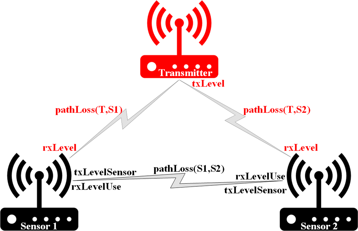
An example structure of sensors and transmitter is presented in Fig. 1.

Fig. 1. Example structure with parameters.
The principal objective in spectrum sensing is the detection of the transmitter signal in the observed band, that consist in a binary decision between a “signal present hypothesis”, named H 1 and a “signal absent hypothesis”, called H 0. The typical detector consists of the evaluation of a particular detection metric, that is computed starting from the observed data, and a threshold comparison which result is the detection decision. The performance of the detection is expressed in terms of probability of false alarm (P FA), that is the probability that the decision metric Λ(y) exceeds the threshold ξ in the hypothesis H 0
 $$P_{FA} = \Pr \{ \Lambda ({\bf y}) \gt \xi \vert H_0 \}, $$
and the probability of detection (P D), that is the probability that the decision metric exceeds the threshold in the hypothesis H 1
 $$P_D = \Pr \{ \Lambda ({\bf y}) \gt \xi \vert H_1 \}. $$
The probabilities P D and P FA are the standard metrics used to evaluate the performance of a detector. In addition, other useful characteristics are the number of samples collected required to reach a particular detection rate and requirements in terms of knowledge of system parameters, minimum SNR for a given performance, use of specific techniques (e.g., oversampling) or equipment (e.g., multiple antennas), etc.
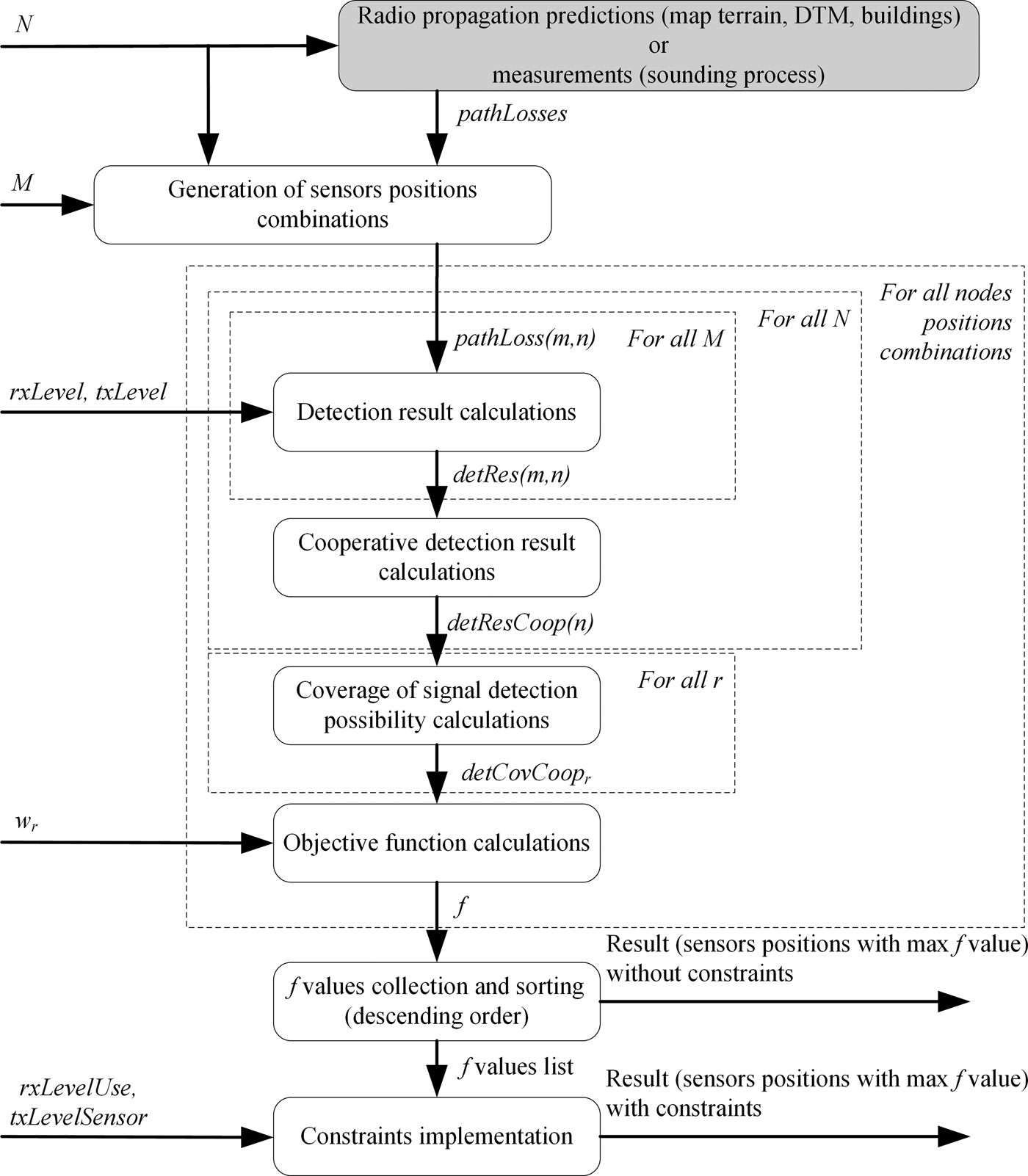
The algorithm of the proposed method is presented in Fig. 2. On the left side, there are input arguments which can be modified in order to investigate their influence on the obtained results (without or with constraints). In the first step, pathLosses values between all defined points should be predicted or measured. After that, all possible sensors positions are determined, depending on N and M. For all these combinations, objective function values f are calculated according to presented above equations (2)–(11) and then sorted in descending order.

Fig. 2. Algorithm of the proposed method.
Tests assumptions
For the purpose of the tests, the urban area with dimensions of 450 m × 420 m was selected (Fig. 3).

Fig. 3. Analyzed area.
Within this region, all potential sensors and radio transmitters locations with the step of 30 m were determined (N = 240 points). The path loss values between all points were calculated by the radio environment module REMO, which was developed within the CORASMA project [Reference Malon, Skokowski, Marszałek, Kelner and Łopatka19]. During the computations, this module takes into account digital terrain model (DTM) and shadowing effect introduced by buildings. Actually, commonly known prediction model (ITM) is used to generate pathLosses values. As a future work, it is planned to verify predicted values with real measurements (sounding campaign). In case of significant differences, adjustments should be added to actual model or another model could be used. It is worth to notice that used model should be selected according to the analyzed terrain.
The considered number of sensors was in the range 1–3.
Results
The conducted research was divided into three sections concerning the influence of:
• detection performance,
• w r coefficients,
• number of sensors and range of communications between them,
on received outcomes.
Influence of detection performance on the objective function values
Many algorithms are proposed for spectrum monitoring with different implementation complexity, detection performance etc. Therefore authors decided not to work out results for a particular method. Instead of that all findings are presented for threshold level (rxLevel) which is universal and transparent for any kind of sensor (matched filter (MF), energy detector (ED), featured based detector (FB), cyclostationary detector or other algorithms derived from the spectral analysis, based, e.g., on multitaper spectral analysis, wavelet transforms or filter banks receivers [Reference McCoy, Walden and Percival20–Reference Yucek and Arslan25]).
In this part objective function (11) values for one sensor is calculated and according to the optimality criterion (14), the maximum result is selected. Figure 4 presents these outcomes versus signal level at the transmitter output (txLevel) for the different received signal level at the sensor input, which enables proper signal detection (rxLevel). Depending on the txLevel and expected area coverage one can see which sensor meets those requirements.
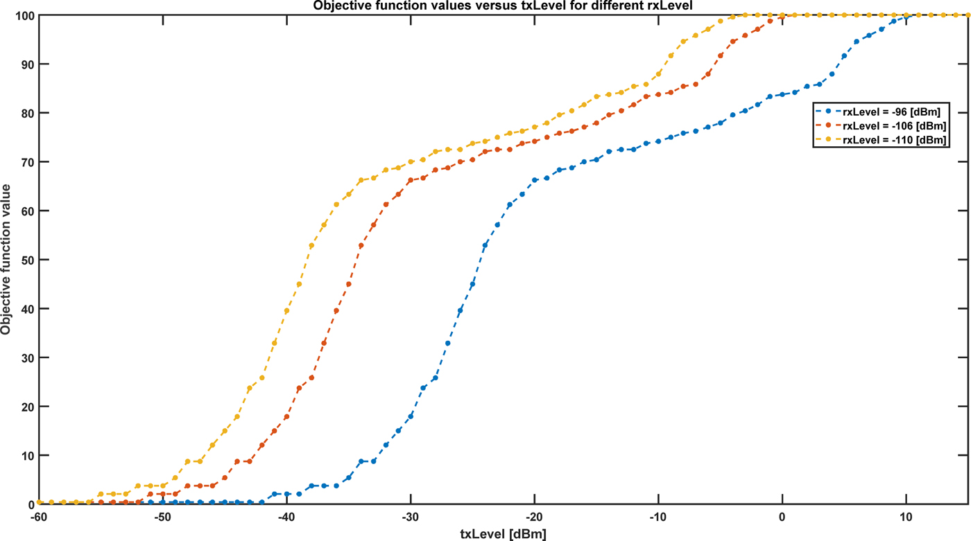
Fig. 4. Maximum objective function values versus txLevel for different rxLevel.
Objective function values for all potential sensors locations for selected rxLevel and txLevel parameters are presented in Fig. 5. Based on the shape of obtained surface authors decide to search the whole space of results to find out global extremum. Usage of other optimization methods might result in stuck in one of the local maxima.
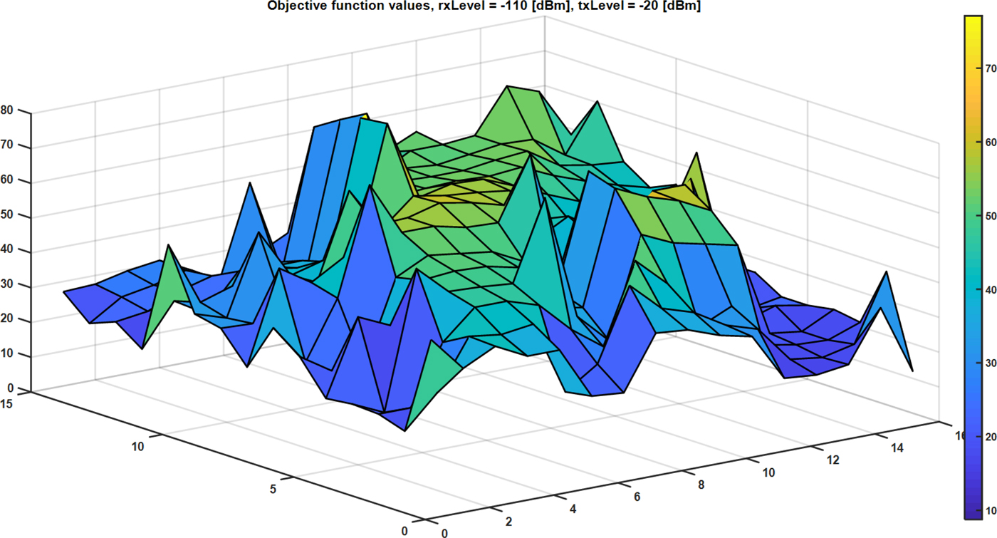
Fig. 5. Objective function values for rxLevel = −110 dBm and txLevel = −20 dBm.
Influence of w r coefficients on the objective function values and sensors deployment without constraints
Results presented in this part (Figs 6–9) show the influence of w r coefficients on objective function values and optimal sensors deployment (colors on the map define redundancy). In this case, constraints relating to the communication range between sensors are not considered. Depending on the demands it is possible to determine nodes locations which satisfy defined requirements. As an example, if it is desirable to maximize the area of detection coverage without redundancy exigency w 1 coefficient shall be set to 1 (Fig. 6). On the other hand, some cases need the higher reliability in spectrum monitoring. Proposed solution address this problem by setting w r coefficients (for r > 1) >0 e.g., w 3 coefficient equal to 1 (Fig. 7). As it can be seen as a consequence of the redundancy requirement some areas cannot be monitored. Those locations might be considered as black zones. Awareness about their existence and location is very important during the sensor network planning process. If such zones are located in critical areas, this knowledge might support the decision to use additional nodes for monitoring. Otherwise, it can be assumed as an acceptable risk.
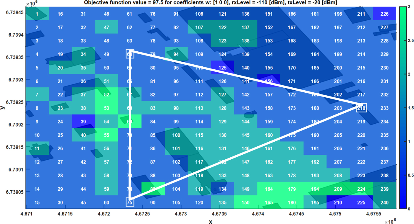
Fig. 6. Optimal sensors locations for coefficients w = [1 0 0], rxLevel = −110 dBm, txLevel = −20 dBm.

Fig. 7. Optimal sensors locations for coefficients w = [0 1 0], rxLevel = −110 dBm, txLevel = −20 dBm.

Fig. 8. Optimal sensors locations for coefficients w = [0 0 1], rxLevel = −110 dBm, txLevel = −20 dBm.
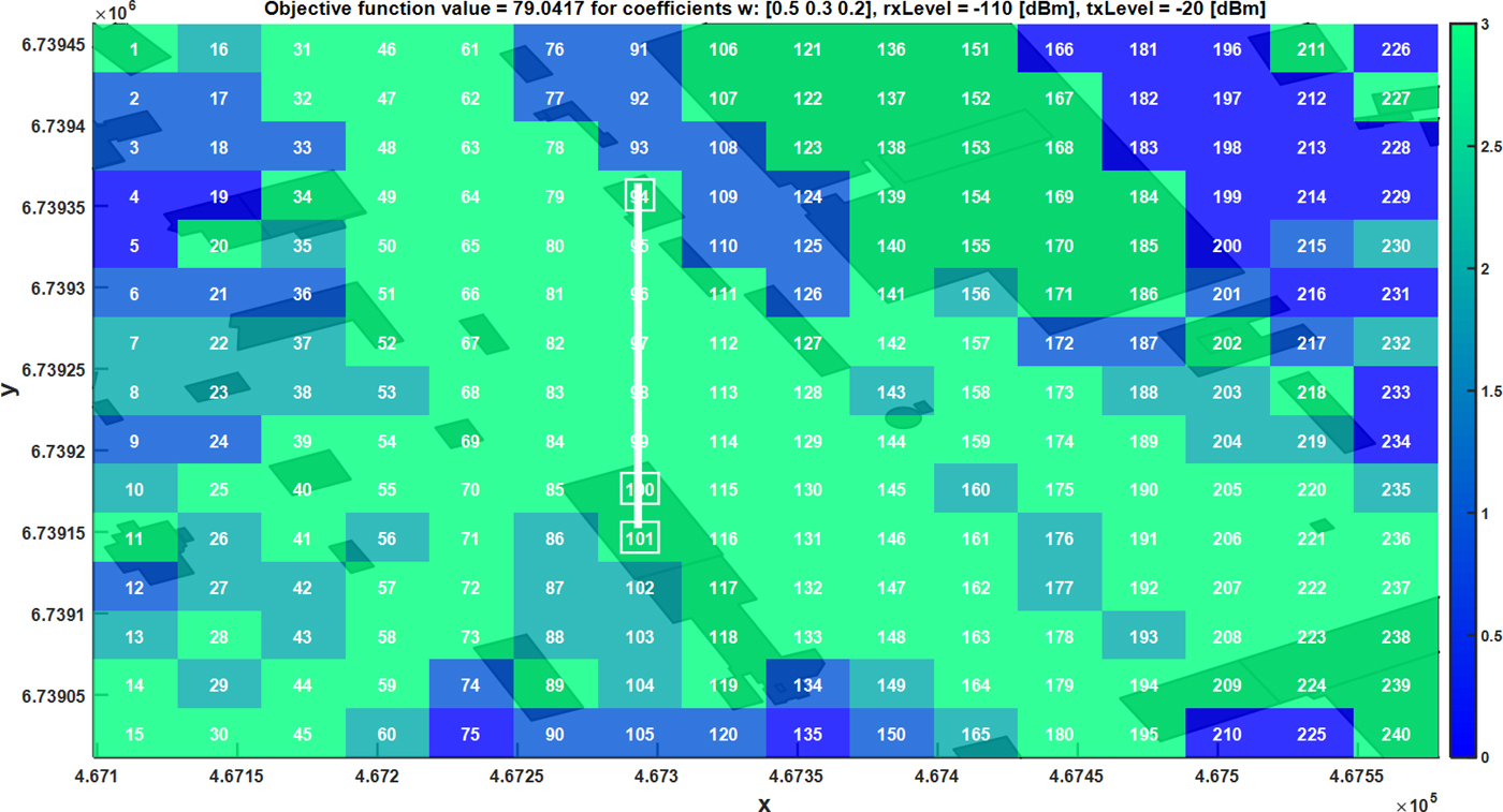
Fig. 9. Optimal sensors locations for coefficients w = [0.5 0.3 0.2], rxLevel = −110 dBm, txLevel = −20 dBm.
Influence of number of sensors on the objective function values without and with constraints
These tests illustrate the influence of sensors number and defined constraints (18) on objective function values. To examine the worst case, the w 1 is equal to 1 and the remaining w r coefficients equal zero. In this case, problems with communication range between sensors are the most probable. Figure 10 presents f function values versus sensorGain defined in (16). As expected, for the case without constraints, increasing the number of sensors results in area coverage growth (f ≈ 77% for one sensor and f ≈ 97% for three sensors). Taking into account limitations specified by formula 18 one can see that f function value depends on sensorGain. Depending on the required area coverage and available number of sensors one can see which receiving and transmitting parameters (sensorGain) meets those expectations. For sensorGain from 54 dB to 60 dB f function curve for two sensors overcome f function curve for three sensors. This is a consequence of the worst case assumption in which communication ranges between all sensors are required. Obviously, it is more difficult to fulfill this condition for a bigger number of sensors.
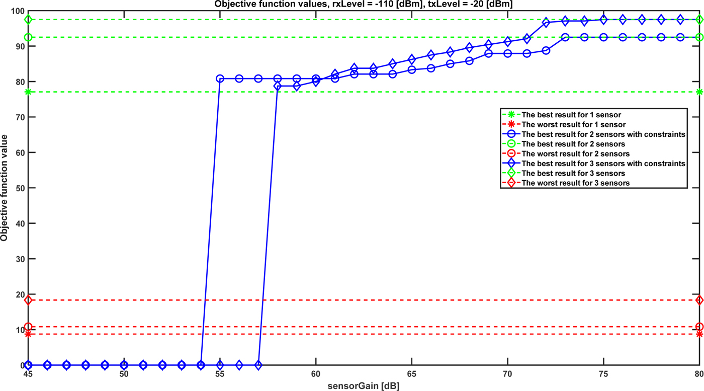
Fig. 10. Objective function values versus sensorGain for rxLevel = −110 dBm, txLevel = −20 dBm.
Conclusion
This paper is devoted to optimization of wireless sensor networks coverage for the purposes of radio spectrum monitoring. It can be also used for electromagnetic situation awareness in cognitive radio networks. Authors propose the methods and criteria to assess the possibility of radio emissions detection by the individual sensors and using the cooperative sensing performed by the group of monitoring nodes. Obtained results depend on terrain shape and assumed propagation model accuracy which are the input data for the presented algorithms.
Influence of the detector performance has been considered as an important factor for monitoring purpose. The area of individual sensors effective operation with limited radio coverage was solved by the use of sensor networks, where the monitoring nodes cooperate with each other in order to elaborate a common result. The problem of finite radio communications range between monitoring nodes is also addressed, with the worst case under consideration.
Elaborated method and metrics have been used for optimal (referring to the f function) nodes deployment which limits the negative effects, such as shadowing or the hidden node problem. Conducted research provides to the conclusion that depending on the demands it is possible to determine zones with various redundancy and to point out priority locations. The advantage of this approach is manifested by an increase in the knowledge of the detection coverage of selected areas which can be adopted for the mission planning process.
Acknowledgment
This work was partially supported by PBS 23-932 project.
 Krzysztof Malon received his MSc degree in Electronics from the Military University of Technology in 2011. He has been participating in many national and international research projects. Currently, he is finishing his Ph.D. degree. His main research interests are wireless communications, cognitive radios, dynamic spectrum access, and radio spectrum monitoring.
 Paweł Skokowski received his MSc degree from the Military University of Technology in 2007. From 2007 has been working at the Telecommunications Institute of MUT as a research assistant. His main research interests are digital signal processing, wireless communications, software-defined and cognitive radio, and electronic warfare. The focus of his work is research, algorithm development and implementation of cognitive and electronic warfare systems. He has been participating in many national and international research projects related to wireless communications and electronic warfare. Currently, he is finishing his Ph.D. degree.
 Jerzy Lopatka received his MSc, Ph.D., and D.Sc. degrees from the Military University of Technology in 1985, 1994, and 2007, respectively. From 2007 has been working at the MUT as a professor. From 2012 until 2016 he was a director of the Telecommunications Institute of MUT. His main research interests are digital signal processing, radio networks, spectrum monitoring, and software defined radio. The focus of his work is design, development and implementation of cognitive radio systems, and electronic warfare systems. He was participating in many national research projects and international EDA projects (ESSOR, ICAR, WOLF, CORASMA) related to wireless communications and electronic warfare. He was also involved in NATO working groups related to cognitive radios and spectrum sharing.