


1. INTRODUCTION
Galileo, Europe's Global Navigation Satellite System (GNSS), was created with the aims of providing positioning, navigation and time services. It was initiated by the European Space Agency (ESA) and the European Commission in the early 1990s, and thereafter, has been a topic of considerable interest within research groups (Furthner et al., Reference Furthner, Moudrak, Konovaltsev and Denks2003; Lindström and Gasparini, Reference Lindström and Gasparini2003; Rodriguez et al., Reference Rodriguez, Hein, Irsigler and Pany2004). The system has been well-maintained in recent years. As of December 2016, the Galileo constellation comprised 18 satellites: four In-Orbit Validation (IOV) satellites, ten Full Operational Capability (FOC) satellites, and four satellites under in-orbit testing (Steigenberger and Montenbruk, Reference Steigenberger and Montenbruck2016). Thus, the preliminary objectives of its establishment have been met. The Galileo system offers one dedicated signal, the broadband signal E5, which is superior to all other available GNSS signals (Simsky et al., Reference Simsky, Mertens, Sleewaegen, Hollreiser and Crisci2008; Diessongo et al., Reference Diessongo, Schüler and Junker2014). However, it is unclear as to how Galileo's time transfer performance may be improved. Additionally, previous studies on Galileo have mainly focussed on positioning and navigation (Angrisano et al., Reference Angrisano, Gaglione, Gioia, Borio and Fortuny-Guasch2013; Diessongo et al., Reference Diessongo, Schüler and Junker2014; Paziewski and Wielgosz, Reference Paziewski and Wielgosz2014).
With respect to precise time transfer, Galileo is comparable to other GNSS, such as the BeiDou navigation system (BeiDou), the Global Positioning System (GPS), and Russia's version of GPS (GLONASS). The Common View (CV) with code measurement is operated frequently in Galileo time transfer, because it can disregard the common errors between the two ground GNSS stations. Previously, simulations of Galileo CV demonstrated a slight performance improvement compared to GPS (Furthner et al., Reference Furthner, Moudrak, Konovaltsev and Denks2003), but the conditions governing the use of CV are greatly limited by the geodetic distance between the two time transfer stations. Compared to the CV technique, the GNSS Carrier-Phase (CP) time transfer technique is able to provide superior results (Schildknecht et al., Reference Schildknecht, Beutler and Rotacher1990; Defraigne et al., Reference Defraigne, Bruyninx and Guyennon2007; Jiang and Lewandowski, Reference Jiang and Lewandowski2012). However, few studies have focused on time transfer based on Galileo CP for one major reason, namely, the lack of available precise Galileo satellite orbit and clock products for CP development since the 1990s. Fortunately, this situation has improved considerably in recent years. In 2012, the International GNSS Service (IGS) began operating the Multi GNSS Experiment (MGEX), which supports newly developed GNSS such as Galileo, BeiDou and the Quasi-Zenith Satellite System (QZSS) (Deng et al., Reference Deng, Ge, Uhlemann and Zhao2014; Uhlemann et al., Reference Uhlemann, Gendt, Ramatschi and Deng2015; Gioia et al., Reference Gioia, Borio, Angrisano, Gaglione and Fortuny-Guasch2015). Several analysis centres, including the European Space Agency (ESA), Deutsches GeoForschungsZentrum Potsdam (GFZ), Centre National d'Etudes Spatiales (CNES), and Center for Orbit Determination in Europe (CODE) provide regular updates of Galileo precise products (Li et al., Reference Li, Ge, Dai, Ren, Fritsche, Wickert and Schuh2015). Therefore, the difficulty posed by the lack of precise orbit and clock products has been overcome, and the prerequisite of time transfer based on the Galileo CP technique can be fulfilled. On the other hand, although the current Galileo constellation consists of 18 available satellites, some, such as satellite E20, still lack measurements in the broadband signal E5. Hence, the number of available Galileo satellites is usually less than four at any observation epoch in many places, which seriously affects the provision of a continuous time transfer service. As shown in Figure 1, the number of available Galileo satellites at every observation epoch during time transfer experiments typically ranges from two to four. Figure 2 presents a typical example of the epoch percentage (65%) of available Galileo satellites (less than four). Thus, the time transfer application based on the Galileo CP technique is hampered by the shortage of available satellites.

Figure 1. The 24 hour ground tracks of the Galileo satellite navigation system on 14 August 2016.

Figure 2. The epoch percentage of available Galileo satellites counted at station NTS1 in China (latitude 34·4°N and longitude 109·22°E) during 14–20 August 2016.
In order to improve the performance of the time and frequency transfer, a new algorithm based on prior information constraints is proposed. A Precise Time Transfer Solution (PTTSol) software package was developed using the algorithm. We have collected a priori information from the station coordinate and troposphere zenith delay, and specific constraint methods have been established. Several experiments were carried out to validate the algorithm in real-time mode and post-processed mode for short baseline and long baseline observations.
The remainder of this manuscript is organised as follows. Section 2 describes the principle of Galileo CP time transfer. Section 3 discusses prior information collection from different aspects in Galileo CP data processing. The details of prior constraint information on the Galileo CP approach, including the mathematical terms and processing strategies, are illustrated in Section 4. Section 5 presents the experimental design used to assess the constraint approaches for Galileo time transfer, and the corresponding results appear in Sections 6, 7 and 8. Section 9 provides discussion and conclusions.
2. THE PRINCIPLE OF GALILEO CP TIME TRANSFER
2.1. Galileo system time
With regard to time and frequency transfer based on Galileo, receivers at different time laboratories are connected to their time and frequency reference points, using one Pulse Per Second (PPS) and 5/10 MHz frequency signals. At each station, the receiver clock is determined by the CP technique, which is the clock difference between the local time scale and Galileo System Time (GST). Therefore, the GST is a bridge between those stations. The GST is a continuous time scale generated by the Galileo Precise Timing Facility (PTF), and the PTF subsystem is equipped with two active hydrogen atomic clocks and four high-performance caesium atomic clocks. The hydrogen atomic clock is characterised by better short-term frequency stability, thus guaranteeing the short-term frequency stability of the GST, as well as frequency stability at the seconds scale for magnitudes of 10−12~10−13. The long-term frequency stability of GST is mainly determined by calculating synthetic atomic time (Hlaváč et al., Reference Hlaváč, Lösch, Luongo and Hahn2006; Hahn et al., Reference Hahn, Achkar, Tuckey, Jones and Pieplu2007).
2.2. The Galileo CP observation model
In general, the ionosphere-free combination can be used for dual-frequency carrier phase and pseudo-range observations in the Galileo CP technique for precise time transfer. They can be expressed as follows:
 $$\left\{\matrix{P = \rho + c(dt_r - dt_s) + T + \varepsilon_P \hfill \cr \Phi = \rho + c(dt_r - dt_s) + T + \lambda N + \varepsilon_\Phi \hfill}\right.$$
where indices s and r refer to the satellite and receiver, respectively; P and Φ denote pseudo-range and CP observations for the ionosphere-free combination, respectively; λ is the wavelength; N is the carrier phase ambiguity; ρ denotes the geometric distance between the phase centre of the satellite and the receiver antenna; c is the velocity of light in vacuum; dt s refers to the satellite clock; and dt r denotes the receiver clock offset, which is the difference between the actual receiver's time system and the GST scale. Considering the existence of hardware delays in the receiver, antenna and cables which convey the internal electrical signal, the receiver clock offset usually contains these hardware delays. Since the delays are stable for a period of time, they can be calibrated with the techniques of relative calibration and link calibration in the area of the time and frequency transfer (Rovera et al., Reference Rovera, Torre, Sherwood, Abgrall, Courde, Laas-Bourez and Uhrich2014; Jiang et al., Reference Jiang, Matsaklis, Zhang, Hector, Dirk and Shinn-Yan2016). T denotes the tropospheric delays, which are independent of the Galileo signal frequency, while εP and εΦ are the multipath effect and measurement noise for pseudo-range and carrier phase observations, respectively.
Tropospheric delay T is usually expressed as the sum of dry and wet components, which can be expressed by their zenith delays and corresponding mapping function. The dry component is usually well corrected by its empirical model, while in the case of the wet component, the zenith delay T wet is set as a parameter to be estimated.
 $$T = {mf}_{dry} \cdot T_{dry} + mf_{wet} \cdot T_{wet}$$
where T dry and T wet denote the dry and wet components of tropospheric zenith delay, respectively, while mf dry and mf wet denote their corresponding mapping functions.
Therefore, the observation equation can be transformed, linearized and given the compact format in Equation (3), and then the parameters to be estimated are summarised in Equation (4):
 $$V = AX - L$$
 $$X = [x, y, z, dt_r, T_{wet}, N]$$
where A is the coefficient matrix of the parameters to be estimated; L denotes “observed minus computed” pseudo-range and carrier phase observations with the ionosphere-free combination; V is the residual vector; X is the parameter vector to be estimated from observations and contains coordinates (x, y, z), receiver clock difference (dt r), tropospheric zenith delay (T wet) and carrier phase ambiguity (N).
3. CURRENT CONSTRAINT INFORMATION FOR TIME TRANSFER
3.1. Station coordinates
For GNSS time transfer, the station remains stationary over a specific time period. Hence, the coordinates of the station can be determined in advance, before the process of time transfer. The positioning accuracy of the station is generally in the centimetre to millimetre range, which does not significantly affect the precise time transfer performance. Therefore, this study introduces precise coordinates for constraint Galileo time transfer, which also allows for a certain amount of errors. The formula can be expressed as follows:
 $$L_c = H_c X_c + e_c$$
where H c is the coefficient matrix of the coordinate, X c is the coordinate vector to be estimated (it contains a three-dimensional component), e c is the corresponding errors vector, and L c is the value of the prior coordinates constraint.
3.2. Troposphere zenith delay
The GNSS signals collected by the GNSS receivers are always affected by the troposphere, by the so-called troposphere delay. This delay is a key issue that affects the validity of time transfer between remote stations, particularly in the CP technique.
From the perspective of atmospheric science, troposphere delay is closely related to environmental temperature, pressure, relative humidity and geodetic height around the station. Fortunately, it is irrelevant to the frequency of remote signals and different GNSS. In this respect, troposphere delay can be set as prior constraint information, which can be determined by other techniques, such as International GNSS Service (IGS) products for troposphere zenith delay. Therefore, the prior constraint mathematical term can be expressed as
 $$L_t = H_t X_t + e_t$$
where H t is coefficient matrix of the troposphere zenith delay, X t is the troposphere parameter to be estimated, e t is corresponding errors vector and L t is the value of the prior troposphere zenith delay constraint.
4. THE MATHEMATICAL MODEL OF THE CONSTRAINT ALGORITHM
The constraint conditions formed by prior information, such as station coordinates and/or troposphere zenith delay, can be used with the original Galileo measurements to estimate the continuous receiver clock. These constraint conditions are equivalent to fixing the value of a station's coordinates and/or troposphere zenith delay to the prior value within a certain range, hence increasing the number of effective observations. When the two a priori pieces of information are applied, the comprehensive mathematical term can be expressed as:
 $$\left[\matrix{L_k \cr L_i} \right] = \left[\matrix{H_k \cr H_i} \right] X + \left[\matrix{e_k \cr e_i} \right]$$
where L k denotes the observation quantity; H k is the coefficient matrix of the observation equation; i denotes the type of constraint, such as station coordinates and/or troposphere zenith delay; L i is the prior value of the constraint information; H i is the coefficient matrix of prior constraints and e k and e i are the corresponding noise errors.
During the data process, the cycle slip of the carrier phase is detected by the geometry-free and Melbourne-Wübbena (Hatch, Reference Hatch1982) model. In the case of coordinates constraint, the initial tropospheric dry delay is corrected by the Saastamoinen (Reference Saastamoinen1972) model, and the wet component is estimated by a random walk process. In the case of the tropospheric delay constraint, the constraint information is formed by IGS tropospheric products. The details of observation models and data processing strategies are listed in Table 1 (Petit and Luzum, Reference Petit and Luzum2010). Here, the interesting parameter of receiver clock offset is estimated by combining pseudo-range and carrier phase observation with a white noise stochastic process (Li et al., Reference Li, Ge, Dai, Ren, Fritsche, Wickert and Schuh2015). In brief, the receiver clock offsets at adjacent epochs are uncorrelated, which is utilised based on the characteristic of atomic clock free running.
Table 1. Observation models and Galileo RINEX data processing strategies.

5. EXPERIMENT DESIGN
In order to assess the performance of precise time transfer by the CP approach with prior constraint information, it is preferable to devise an experiment focused on the time link length. Stations USN8 and USN9 (located at the United States Naval Observatory (USNO)) are equipped with the common UTC (USNO), while Station NTS1 (located at the National Time Service Center (NTSC)) is linked to the UTC (NTSC). The details of these three stations are listed in Table 2. In this case, two time links can be established. The first time link, USN9-USN8, is equipped with the common UTC (USNO) and antenna at the short baseline. In this situation, the clock difference only contains some hardware delays that are stable in the short term and this can also provide an external reference to verify the time transfer performance. The second is the NTS1-USN8 link spanning over 10,232 km, which presents a long baseline time link.
Table 2. Detailed information of the three stations used for the experiments in this study.

Considering that poor accuracy of the prior constraint's information will distort the performance of the CP constraint approach, the corresponding accuracy must be guaranteed. Therefore, the prior coordinate's information is used from the post Precise Point Positioning (PPP) solution, because it is superior to the real-time solution when the convergence arc is removed by a backward and forward Least Squares (LSQ) estimator in sequential modes. Then, the three stations’ coordinates were provided by GPS three-day PPP solutions, and the accuracy was found to be better than 1 cm in the horizontal component and 2 cm in the vertical component. In the following sections, “Coord” denotes the approach of combining only the coordinate information and observations. With respect to the troposphere zenith delay, it is also determined by GPS post PPP solutions. The accuracy of the troposphere is superior to 2 cm for the three stations. In approach “Trop”, only the troposphere zenith delay constraint is used. “C+T” refers to constraining the prior information of both the station coordinates and troposphere zenith delay. “Raw” denotes the Galileo classical CP transfer approach, in this, prior constraint information is not used.
Two different data processing modes (real-time and post-processed) are explored in this study of precise time transfer improvements. Note that the prior constraint information is determined in post mode, which is only used for the sake of ensuring its accuracy. When the two processing modes are referred to the CP constraint approach, we assume that the different performance between the two modes can only come from the CP constraint approach. Regarding the analysis of time transfer in real-time mode, the convergence criterion is defined as a positioning error of less than 0·1 m. In the post-processed mode, the parameters are estimated by backward and forward LSQ in sequence, in which the convergence arc can be removed.
6. RESULTS FOR THE SHORT BASELINE TIME LINK
The time link is usually equipped with two different external time and frequency references at the two ends of the time link. However, since the two references have different characteristics, it is difficult to assess the performance of the approach that is employed to determine the clock difference. Meanwhile, the clock difference contains not only the values of time transfer but also the hardware delays from Galileo receivers, antennae and cables. In order to assess the accuracy of the time transfer approach, a short baseline time transfer scheme is employed, in which a common external time and frequency reference is used. Therefore, the time transfer value only contains hardware delays of the Galileo receivers and antennae, and this component is used to assess if the proposed approach is theoretically relatively stable in the short term. The Receiver Independent Exchange Format (RINEX) data of USN8 and USN9 were obtained on 14 August 2016 from the MGEX network. Considering the close distance between USN8 and USN9, Figure 3 presents the available number of satellites that were tracked by NTS1 and USN8 on that day.

Figure 3. The available number of satellites that were tracked by NTS1 and USN8.
6.1. Real-time mode
Figure 4 shows the real-time clock difference between USN8 and USN9 for the four approaches based on Galileo carrier phase observations. The statistical information on real-time clock difference is listed in Table 3, and the Allan deviation is given in Figure 5 and Table 4. It can be seen that the approaches with prior constraint information have obviously ameliorated the issues with time transfer. For the standard CP, the convergence time is much longer than the approaches with prior constraint information. Compared with the standard Galileo CP for precise time transfer, the Standard Deviation (STD) improved by 51·4% for the troposphere zenith delay constraint, 47·6% for the station coordinates constraint, and 49·5% when considering both constraints simultaneously.

Figure 4. The real-time clock difference between USN8 and USN9 for the four approaches in real-time mode.

Figure 5. Comparison of the Allan deviations for the four approaches in real-time mode for USN8-USN9.
Table 3. The statistical results of the short baseline time link in real-time mode (unit: ns).

Table 4. Value of the Allan deviations for the four methods in real-time mode for USN8-USN9.

6.2. Post-processed mode
Figure 6 illustrates the post-processed mode clock difference between USN8 and USN9 for the four approaches. The statistical information of the post-processed mode clock difference is listed in Table 5, and the Allan deviation is given in Figure 8 and Table 6. An accuracy of 0·023 ns can be achieved for the standard Galileo CP time transfer in the short baseline time link, which is comparable to GPS. As the backward and forward LSQ in a sequential estimator is employed in post-processed Galileo time transfer, the unknown parameters can be estimated accurately. Therefore, the superiority of prior information approaches is not significant, and in some cases, even the prior information may introduce certain errors in accuracy levelling. The results of the “Trop” approach are in agreement with that of the “Raw” approach. A comparison of “Coord,” “T+C,” and “Raw” shows that the station coordinates constraint could cause a certain slope in clock difference, a finding that is in accordance with previous studies on GPS CP time transfer (Yao and Levine, Reference Yao and Levine2012). In order to investigate the sensitivity of how the stations’ coordinate components affect the performance, a short analysis was employed. When an additional 1 m error was added to the station coordinate components (x, y, z), the corresponding average values of the clock differences were temporarily determined and could be compared with the coordinate constraint solution without the extra 1 m error. The relative average distortion percentages of these coordinate components are shown in Figure 7. It can be seen that the y-component has the most distorted clock difference slope. Therefore, we can conclude that the accuracy of y-components is more important in time transfer when the station coordinate constraints are used.

Figure 6. The clock difference between USN8 and USN9 for the four approaches in the post-processed mode.

Figure 7. The distortion percentages of the three coordinate components.

Figure 8. Comparison of the Allan deviations for the four approaches in post-processed mode for USN8-USN9.
Table 5. The statistical results of the short baseline time link in post-processed mode (unit: ns).

Table 6. Value of the Allan deviations for the four methods in post-processed mode for USN8-USN9.
7. RESULTS FOR THE LONG BASELINE TIME LINK
Long baseline time link requirements usually need to be met in applications of precise time transfer. Thus, it is necessary to test the effectiveness of the proposed method for such cases. The RINEX data of NTS1 and USN8 were obtained on 14 August 2016. The time link for USN8-NTS1 is about 10,232 kilometres apart. Similarly, the two data processing modes of Galileo CP are also used for determining the clock difference for the time links. Given the clock difference between the two stations (which are equipped with different external time frequencies), it is crucial to ascertain the accuracy/suitability of the proposed approaches with regard to the time frequency information. Thus, Allan deviation is employed to assess the performance of time transfer for different average times.
7.1. Real-time mode
Figure 9 shows the real-time clock difference for link USN8-NTS1 for the four approaches. It is obvious that three approaches with prior constraint information show less variation than the standard Galileo CP technique in real-time mode, especially before the full convergence of the standard Galileo GP. Regarding the “Coord” and “T+C” approaches, the station coordinates could also contribute to the slope in time transfer. Since the clock difference series is not fully convergent from epoch 500 onward, the Allan deviation from epoch 500 backward is given in Figure 10 and Table 7, which is at different time intervals for each CP approach for the USN8-NTS1 time link in real-time mode. Note that the approaches with prior constraint information show findings similar to the standard CP at time intervals of 30 s, 60 s, 120 s, 240 s, 480 s and 960 s. However, once the time interval exceeds 1,000 s, the approaches become superior to the standard CP time transfer. At the 10,000 s time interval, in comparison to the standard CP, the three constraint approaches show stable results as well as improvements of nearly an order of magnitude.

Figure 9. The real-time clock difference for link USN8-NTS1 for the four approaches.

Figure 10. Comparison of the Allan deviations for the four approaches in real-time mode for USN8-NTS1.
Table 7. Value of the Allan deviations for the four methods in real-time mode for USN8-NTS1.

7.2. Post-processed mode
Figure 11 shows the clock difference for link USN8-NTS1 for the four approaches in post-processed mode. It can be seen that the clock differences determined by the four approaches agree well with one another. The station coordinates constraint still leads to the slope from the ‘Coord’ and the ‘T+C’ approaches. In addition, the ‘Coord’ and ‘T+C’ are highly correlated, and then correlation coefficient reaches 0·99 for the USN8-NTS1 link in post-processed mode. This correlation can be attributed to the accuracy estimation of troposphere zenith delay in post-processed mode. Figure 12 and Table 8 illustrate the Allan deviation values at different time interval for each of the four CP approaches for time link USN8-NTS1 in post-processed mode. It can be seen that the values obtained from any constraint approaches at every time interval have slight improvements compared to the standard Galileo CP.
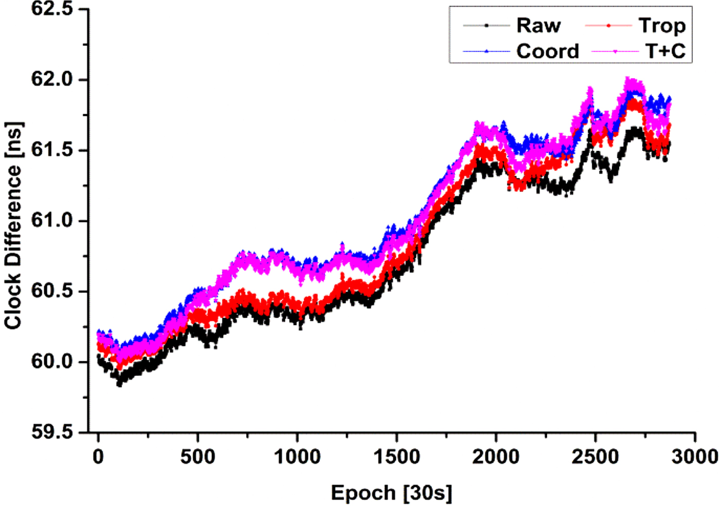
Figure 11. The clock difference for link USN8-NTS1 for the four approaches in post-processed mode.

Figure 12. Comparison of the Allan Deviations for the four approaches in post-processed mode for USN8-NTS1.
Table 8. Value of the Allan Deviations for the four approaches in post-processed mode for USN8-NTS1.

8. RESULTS FOR FIVE-DAYS’ TIME TRANSFER
In Sections 6 and 7, we have indicated that the CP approaches with prior constraint information can improve the performance of time transfer, particularly in real-time mode. In order to further verify the performance, the new approach was validated by an additional five days’ data in real-time mode, from 18–22 August 2016. Both the short and long baseline links were tested. Figure 13 shows the clock difference of the short baseline time link; the corresponding statistical information after full convergence is given in Table 9, and the Allan deviation is shown in Figure 14 and Table 10. With respect to the long baseline time link, the corresponding clock difference is shown in Figure 15 and the Allan deviation is given in Figure 16 and Table 11. It also can be seen that the CP approaches with prior constraint information can improve the time transfer performance.

Figure 13. The clock difference of five days' time transfer for link USN8-USN9 by four different approaches.

Figure 14. Comparison of the five days' Allan deviations for link USN8-USN9 by four different approaches.

Figure 15. The clock difference of five days' time transfer for link USN8-NTS1 by four different approaches.

Figure 16. Comparison of the five days' Allan deviations for link USN8-NTS1 by four different approaches.
Table 9. The five days' statistical results of the short baseline time link (unit: ns).

Table 10. Value of the five days' Allan deviations by four different approaches for USN8-USN9.

Table 11. Value of the five days' Allan deviations by four different approaches for USN8-NTS1.

9. DISCUSSION AND CONCLUSIONS
This study developed the approaches for improving Galileo CP time transfer by applying station coordinates and tropospheric zenith delay information, which are determined by the GPS post-processed solution. Then, the approaches were applied to real-time and post-processed modes for short baseline and long baseline time links. The validations lead to the following conclusions.
In terms of real-time and precise time transfer, the prior constraint information CP approaches showed significant improvement compared to standard Galileo CP. For the short baseline time link, the constraint approaches obviously exhibited less variation than standard CP with regard to clock difference. In addition, the standard deviation improved by 51·4% when considering the troposphere zenith delay constraint, and 47·6% and 49·5%, respectively, when considering the station coordinates constraint and both constraints. Regarding the long baseline time link, the constraint approaches showed less variation, and the Allan deviations indicated significant improvements when the time interval was longer than 10,000 s. These results indicate that the time transfer performance can be significantly improved by these constraint approaches in the real-time mode; the same conclusion can also be reached from the five days’ time transfer experiment.
For the post-processed and precise time transfer, the STD value of standard Galileo CP time transfer is 0·023 ns for the short baseline time link when the sampling period is 30s, which is comparable to that of GPS. Because the convergence session of the standard CP approach was removed in the post-processed mode, and the unknown parameters were estimated consistently, the superiority of the constraint CP approach was not obvious. For the short baseline time link, a standard deviation of 0·025 ns was achieved with the troposphere zenith delay constraint, and the corresponding values were 0·056 ns for the station coordinates constraint and 0·057 ns for both constraints. With respect to the long baseline time link, the Allan deviations showed a similar trend and there was little difference among the approaches at different time intervals. Therefore, the constraint approaches exhibited significant improvement in real-time mode Galileo CP time transfer compared to the post-processed mode.
Different constraint information elements showed distinctive performance with regard to time transfer. Although the method employed only one constraint condition for troposphere zenith delay and three constraint conditions for station coordinates, the real-time result of the approach showed that the standard deviation was in agreement with that of the station coordinates approach. Meanwhile, in the post-processed mode, the troposphere zenith delay constraint resulted in a 0·025 ns standard deviation for a short baseline time link, which is superior to the corresponding station coordinates constraint approach (0·056 ns). This finding can be attributed to the fact that the station coordinates constraint easily leads to the slope in clock difference. Moreover, the results for the short baseline time link showed that when the troposphere zenith delay parameter was constrained, the extra station coordinates constraint approach could not significantly improve the results in both the real-time and post-processed modes. Therefore, the troposphere zenith delay constraint was more capable of achieving precise CP time transfer than the station coordinates constraints.
Given the rapid developments with the Galileo satellite navigation system, it is likely that the pace of research on this topic will increase. As the accuracy and stability continue to be improved, use of the Galileo time link will eventually be expanded to computing Coordinated Universal Time (UTC).
ACKNOWLEDGEMENTS
We are very grateful to MGEX for providing Galileo data. The work was partly supported by the program of National Key Research and Development Plan of China (Grant No. 2016YFB0501804), National Natural Science Foundation of China (Grant No. 41504006, 41674034) and Chinese Academy of Sciences (CAS) programs of “Pioneer Hundred Talents”, Light of the west joint scholar” (Grant No. Y507YR1201) and “The Frontier Science Research Project” (Grant No. QYZDB-SSW-DQC028), National Time Service Center (NTSC) programs of “Young creative talents” (Grant No. Y824SC1S06).


