I. Introduction
The modern presentation of the law of one price (LOOP) is credited to Cassel (Reference Cassel1918) and has sometimes been called the “second law of economics” (Biondo, Reference Biondo2010; Lamont and Thaler, Reference Lamont and Thaler2003). LOOP is often seen as a reflection of market efficiency. After transaction cost, arbitrage should ensure price convergence between different markets. Deviation from LOOP can be due to various factors, such as trade barriers, institutional differences, producers' or sellers' strategic behavior, and so forth. However, such deviations are expected to be small on financial markets, because financial assets are homogenous and immediately tradable, at nearly no cost, and arbitrageurs can correct prices differences instantaneously. However, even in financial markets, some anomalies can occur, raising the question of the validity of the price signal sent to investors (Lamont and Thaler, Reference Lamont and Thaler2003). In general, distorted price signals can lead to misallocations of investments and thus destabilize financial asset markets, including fine wines.
The emergence of fine wine as an alternative asset class during the 2000s gives rise to shedding light on wine-portfolio valuation and investor information. Liv-ex provides several fine-wine indices based on a mix of current transaction prices (from affiliated merchants and auction prices), which are frequently used by investment funds and researchers (for a literature survey, see Storchmann, Reference Storchmann2012). Wine-investment funds often disregard potential price dispersion as well. For instance, the Luxembourg-based fund Grands Crus simply calculates the end-month price of any bottle in its portfolio as the average of four prices from a list of sixty wine merchants and ten auction houses. If prices were systematically skewed and did not follow LOOP, such a pricing method may convey incorrect signals to investors.
This paper is aimed at identifying deviations from LOOP in the fine-wine market and assessing their origins and magnitudes.
Several methods have been used to test LOOP in various contexts, such as financial markets, commodity markets, final-consumption goods,Footnote 2 retail prices,Footnote 3 production prices, and so forth. We distinguish two LOOP versions. The strong version postulates perfect price equality for the same good/asset sold in two different places at the same time (taking into account transaction costs). The strong version holds only if arbitrage is immediate and is thus often rejected. The weak version requires only convergence, or at least a co-movement in prices, of identical goods sold in different markets. Co-integration analysis is then often used to verify the weak version of LOOP. Even this weak version receives only mixed support in the extensive literature on LOOP (Lamont and Thaler, Reference Lamont and Thaler2003).
For alternative investments, especially in art markets, several authors find deviation from LOOP (e.g., Ashenfelter and Graddy, Reference Ashenfelter and Graddy2003; Pesando, Reference Pesando1993; Pesando and Shum, Reference Pesando and Shum2007).
Only a few studies have analyzed LOOP on the wine market. Ashenfelter (Reference Ashenfelter1989) finds LOOP deviations in wine auctions,Footnote 4 mainly due to the “declining price anomaly.” Ginsburgh (Reference Ginsburgh1998) investigates this anomaly over four wine auctions at Christie's London. Both authors identify buyers' risk perception as the reason for the price-decrease phenomenon during auctions. More recently, Jaeger and Storchmann (Reference Jaeger and Storchmann2011) draw on a large database of U.S. retail wine prices and find significant deviations from LOOP, especially for expensive wines.
Our analysis examines the strong version of LOOP on the global auction market for fine wine. We draw on a large international auction-price database taken from numerous auction houses with worldwide auctions held between 2000 and 2012. Our analysis focuses on the five Bordeaux first-growth wines that are included in the Liv-ex 50 index (i.e., Haut-Brion, Lafite Rothschild, Latour, Margaux, and Mouton Rothschild). These wines are among the most-traded and sought-after wines by many investors. If LOOP is violated for these relatively liquid wines, the effect is likely to be more pronounced for less liquid/traded wines (Roll, Schwartz, and Subrahmanyam, Reference Roll, Schwartz and Subrahmanyam2007). Finally, auction data are commonly used for wine-related academic research (e.g., Burton and Jacobson, Reference Burton and Jacobsen2001; Fogarty, Reference Fogarty2010; Jones and Storchmann, Reference Jones and Storchmann2001; Masset and Weisskopf, Reference Masset and Weisskopf2010; Sanning, Shaffer, and Sharratt, Reference Sanning, Shaffer and Sharratt2008; for a literature survey, see Storchmann, Reference Storchmann2012). Auction-house data are also less sensitive to pricing-to-market behavior than are national-merchant data. The fine-wine auction market is global, with few actors and similar settlement fees. Thus, compared to merchant data, wine-auction data resemble conventional financial data.
We find that the price ranges for most wines far exceed the transaction costs, suggesting the existence of substantial price dispersion, which is only partially explained by the heterogeneity of some sales. Running a hedonic quantile regression model with various regional interactions, we find that auction prices in Hong Kong are significantly higher than elsewhere. In particular, young wines with high critical scores attain higher prices in Hong Kong than elsewhere. In addition, there are higher premiums for sales of full cases of twelve bottles and for wines by Château Lafite Rothschild, indicating some orientation toward prestige wines. Our results also suggest the existence of Hong Kong price premiums for wines that are deemed counterfeit suspects on the Internet and sell at discounted prices in Europe and the United States.
The remainder of this paper is organized as follows: Section II presents the data and the methodology. Section III compares price ranges and transaction costs of certain wines to isolate wines that potentially violate LOOP. Section IV includes our hedonic model and our results. The final section concludes.
II. Data and Methodology
A. Descriptive Statistics
We draw on price data for all five Bordeaux first growths from the Wineprices website.Footnote 5 Prices are per bottle (750mL) in U.S. dollars (USD). We convert sales in other currencies to USD using the sale date's exchange rate. We only consider uniform lots with identical wines (same producer and vintage) and disregard mixed lots. All prices include the respective buyer premiums but exclude sales taxes or value-added tax (VAT). Auction results come from several auction houses over the period from 2000 to 2012, representing almost the entire fine-wine auction market by volume and number of transactions.Footnote 6 Our original dataset comprises 79,661 wine transactions, representing 662,652 standard bottles (750mL) with a total sales value of US$457 million.
Like in the Liv-ex 50, we consider the five grands crus châteaux of Bordeaux (Haut-Brion, Lafite Rothschild, Latour, Margaux, and Mouton Rothschild). However, and in contrast to the Liv-ex 50, which includes only the last ten vintages, we also include older wines and draw on most vintages from 1945 to 2009. Figure 1 shows that most auction sales focus on only a few vintages (particularly 1982, 1986, 1989, 1990, 1995, 1996, and 2000), which gives rise to two problems. First, price differences are statistically significant only if we compare sufficiently large sub-samples for different locations. Second, weakly traded vintages are unattractive for investors seeking a liquid market.

Figure 1 Number of Transactions by Vintage
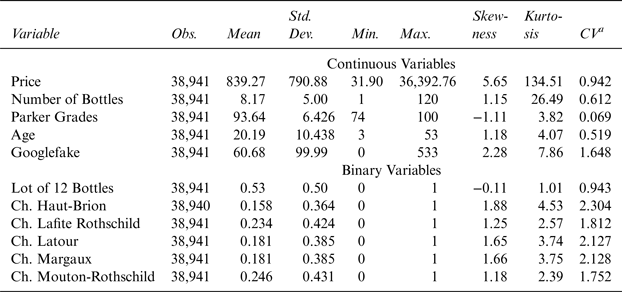
Due to limited availability, we find significantly fewer transactions of wines from vintages prior to 1982. To also include older vintages from before 1982, we proceed as follows. First, we divide our sample into two periods, Period 1 (vintages 1945–1981) and Period 2 (vintages 1982–2008). Employing Fischer's algorithm, we then partition each sub-period into three classes (Appendix Table A1) and retain only the ten most frequently traded vintages (which are part of the third interval of each period). This sub-sample comprises 38,941 observations. Table 1 provides the descriptive statistics of the continuous variables; Figure 2 through 7 show the number of transactions over time, by company, by location, and by château.
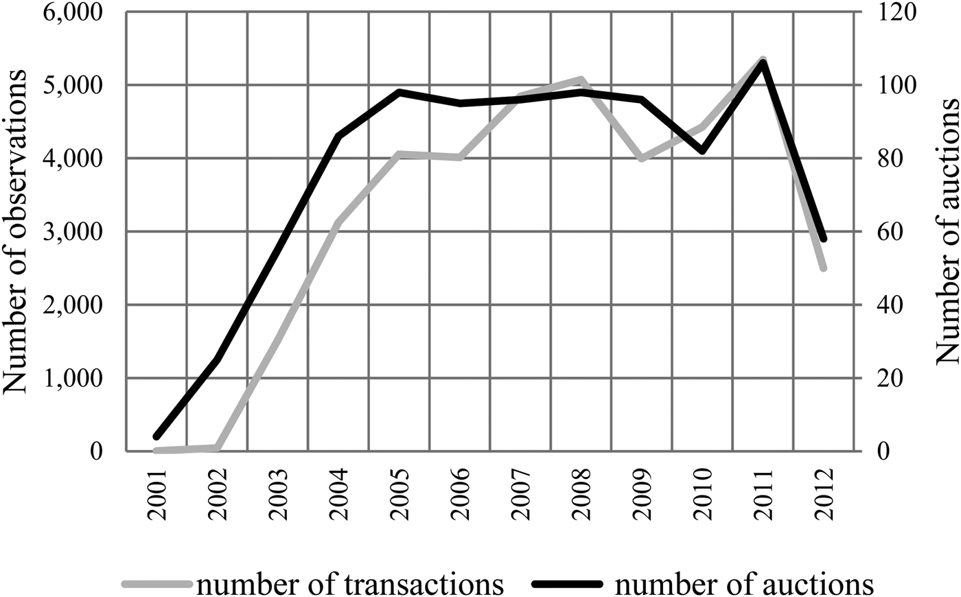
Figure 2 Number of Auctions and Transactions by Year
Table 1 Descriptive Statistics of Selected Variables

a The Coefficient of Variation (CV) is defined as the standard deviation divided by the mean
![]() $CV = \displaystyle{\sigma \over \mu} $
.
$CV = \displaystyle{\sigma \over \mu} $
.
Figure 2 shows the take-off of the fine-wine auction market in the early 2000s. The rise is mainly due to an increase in the number of auctions and of independent auction houses, while the number of transactions per auction remains relatively stable.
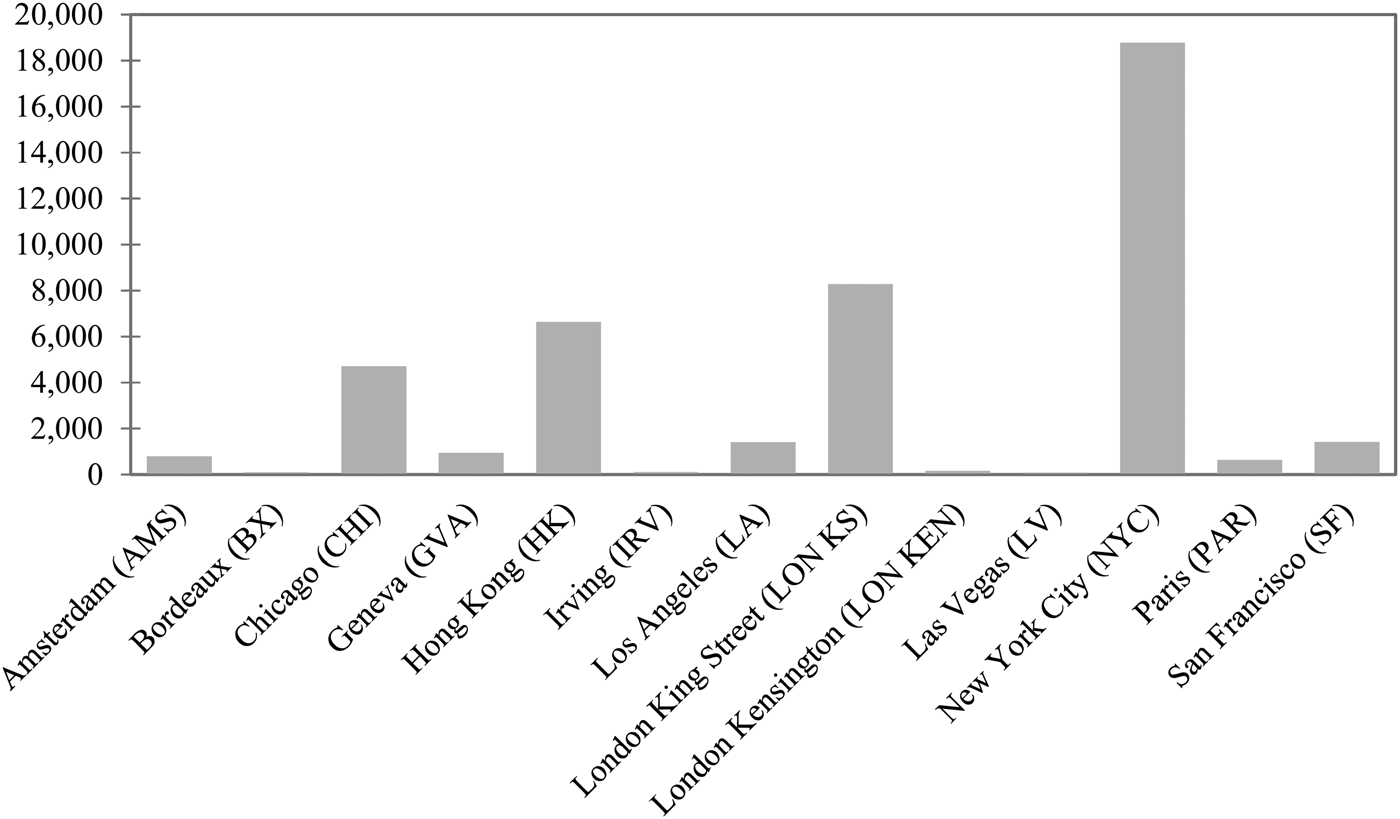
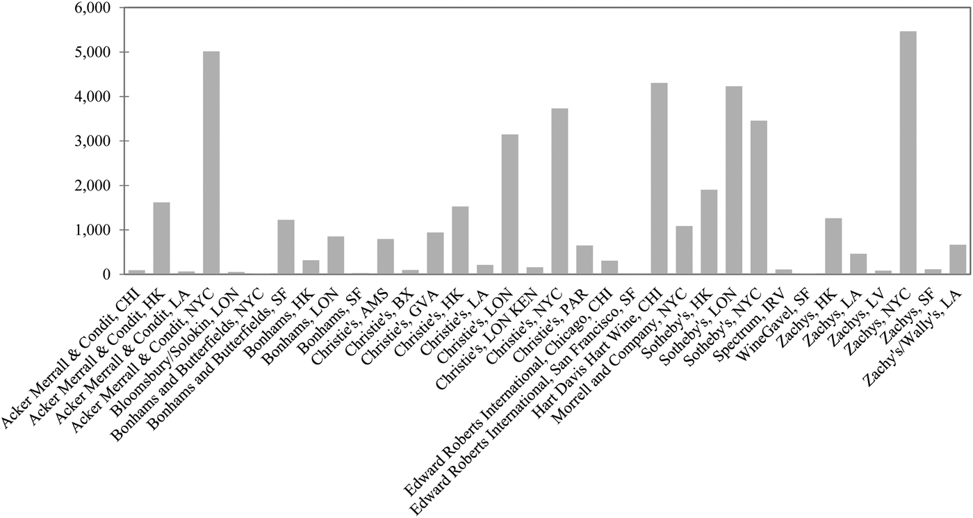
Of the auction companies in our sub-sample, the largest four (i.e., Christie's, Sotheby's, Zachys, and Acker Merrall & Condit) account for approximately 80 percent of all transactions (Figure 3). These companies sell in ten cities (i.e., Amsterdam, Bordeaux, Chicago, Geneva, Hong Kong, London, Los Angeles, New York, Paris, and San Francisco). Figure 4 shows the predominance of New York, ahead of London and Hong Kong; the latter has become a major market only since 2008. Combining companies and places allows us to identify numerous auctions of differing weights in the global auction market (Figure 5). Finally, Figure 6 reports the number of transactions by château and shows a slight predominance of the “two Rothschilds,” Lafite and Mouton.
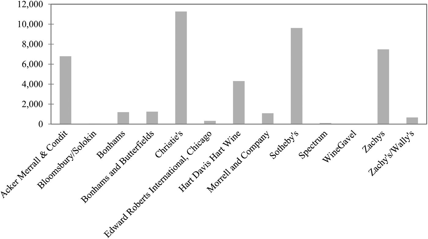
Figure 3 Number of Transactions by Auction Company

Figure 4 Number of Transactions by Location

Figure 5 Number of Transactions by Auction Company and Location
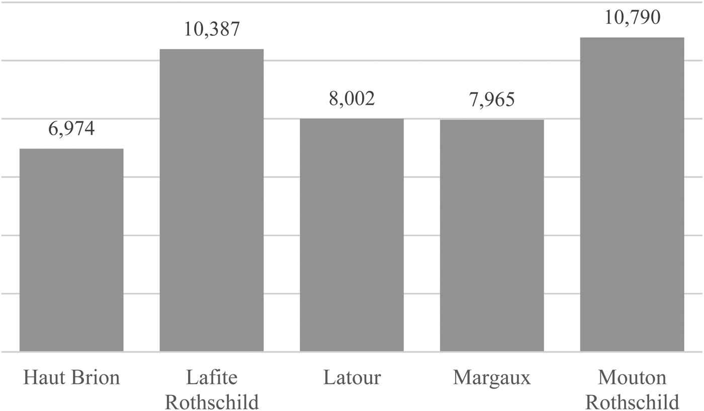
Figure 6 Number of Auctions by Château
B. LOOP and Methodology
Various methods have been used in the literature to test the strong and weak versions of LOOP. Suppose two marketplaces, A and B, trade the same good/asset. Assuming arbitrage, the strong version implies that contemporaneous prices of this good/asset are equal after controlling for transaction costs:
where
![]() $P_t^A $
(
$P_t^A $
(
![]() $P_t^B $
) is the price of the good/asset in market A (B) at time t, and
$P_t^B $
) is the price of the good/asset in market A (B) at time t, and
![]() $C_t^B $
represents the transaction cost in market B at time t.
$C_t^B $
represents the transaction cost in market B at time t.
The weak form only requires some degree of price convergence (i.e., a price change in A should induce a price change in B). Consider equation (2):
where ΔP
t
= P
t
− P
t−1, and u
t
is the i.i.d. error term. LOOP is confirmed if α = 0 and β = 1. The weak form of LOOP requires only the long-term convergence of
![]() $P_t^A $
and
$P_t^A $
and
![]() $P_t^B $
and does not stipulate strict price equality.
$P_t^B $
and does not stipulate strict price equality.
We approach our research object from various angles. First, we compare the price ranges for certain wines with their corresponding transaction costs at various auction places and time periods. Ideally, we want to compare sales at different locations that occur at the same time. However, compared to stock prices, the database for wine-auction prices is rather thin. We thus designate quarters as the time unit.
We then examine whether auction mechanisms or wine heterogeneity may be a possible price-dispersion driver.
Finally, we augment the analysis with an annual hedonic quantile regression panel model that includes various country interactions of the most relevant variables to examine the existence of regional price dispersion.
III. Average-Price and Transaction-Cost Analyses
This paper analyzes château-vintage price dispersion within and between auctions. To ensure the comparability of each auction company's sub-sample, some data restructuring is required. We only retain the most liquid vintages (1982, 1986, 1989, 1990, 1995, 1996, and 2000) and nine auctions (accounting for about 80 percent of all transactions) at Acker Merrall & Condit (New York), Christie's (Hong Kong, London, and New York), Hart Davis Hart Wine Co. (Chicago), Sotheby's (Hong Kong, London, and New York), and Zachys Wine Auctions (New York).
To examine differences, prices should ideally be observed at the same time. However, in contrast to financial markets, fine-wine auctions do not produce enough data points to warrant an analysis based on daily price data. Therefore, as a compromise between data availability and comparability, we choose to work with quarterly data and cover the time from the first quarter (Q1) of 2003 to the third quarter (Q3) of 2012.
We use a dispersion indicator comparing the maximum and minimum prices observed within each individual auction (
![]() $m_w^{ij} $
) or among all the auction companies considered (
$m_w^{ij} $
) or among all the auction companies considered (
![]() $m_b^i $
) for each château vintage i:
$m_b^i $
) for each château vintage i:
 $$m_w^{ij} = \; \displaystyle{1 \over K}\; \mathop \sum \nolimits_{k = 1}^K \left( {\displaystyle{{P_{max_j}^k} \over {P_{min_j}^k}}} \right)\,{\rm and}\,\,m_b^i = \; \displaystyle{1 \over N}\; \mathop \sum \nolimits_{t = 1}^N \left( {\displaystyle{{P_{max}^t} \over {P_{min}^t}}} \right).$$
![]() $P_{max_j}^k $
is the maximum price observed in the single auction k in auction company j;
$P_{max_j}^k $
is the maximum price observed in the single auction k in auction company j;
![]() $P_{min_j}^k $
is the minimum price observed in the single auction k in auction company j;
$P_{min_j}^k $
is the minimum price observed in the single auction k in auction company j;
![]() $P_{min}^t $
is the minimum price observed during quarter t,
$P_{min}^t $
is the minimum price observed during quarter t,
![]() $\forall j$
;
$\forall j$
;
![]() $P_{max}^t $
is the maximum price observed during quarter t,
$P_{max}^t $
is the maximum price observed during quarter t,
![]() $\forall j$
;
$\forall j$
;
![]() $m_w^{ij} $
is the within auction indicator, where k = 1,…,579 represents the individual auction (579 is the total number of auctions during the Q1 2003 to Q3 2012 period for the eleven auction companies we have selected); i denotes the château-vintage pair (i = 1,…,35); and j stands for the auction company (j = 1,…,11).
$m_w^{ij} $
is the within auction indicator, where k = 1,…,579 represents the individual auction (579 is the total number of auctions during the Q1 2003 to Q3 2012 period for the eleven auction companies we have selected); i denotes the château-vintage pair (i = 1,…,35); and j stands for the auction company (j = 1,…,11).
![]() $m_w^{ij} $
measures the average maximum price dispersion within a single auction over the entire period, for any château-vintage pair i. This indicator (within) is then calculated for each auction house j (see Appendix Table A2 and A3).
$m_w^{ij} $
measures the average maximum price dispersion within a single auction over the entire period, for any château-vintage pair i. This indicator (within) is then calculated for each auction house j (see Appendix Table A2 and A3).
![]() $m_b^i $
is the between auction house indicator and measures the average maximum price dispersion between auctions during a quarter when the maximum and minimum prices occur.
$m_b^i $
is the between auction house indicator and measures the average maximum price dispersion between auctions during a quarter when the maximum and minimum prices occur.
Table 2 provides the descriptive statistics on quarterly average price ratios within (
![]() $m_w^{ij} $
) and between (
$m_w^{ij} $
) and between (
![]() $m_b^i $
) auction houses. The resulting asymmetric and leptokurtic distributions of the ratios shed doubt on the existence of LOOP.
$m_b^i $
) auction houses. The resulting asymmetric and leptokurtic distributions of the ratios shed doubt on the existence of LOOP.
Table 2 Descriptive Statistics of Within and Between Dispersion Indicators

Within dispersion indicator
![]() $m_w^{ij} \; \; $
and between dispersion indicator
$m_w^{ij} \; \; $
and between dispersion indicator
![]() $m_b^i $
; see also equation (1).
$m_b^i $
; see also equation (1).
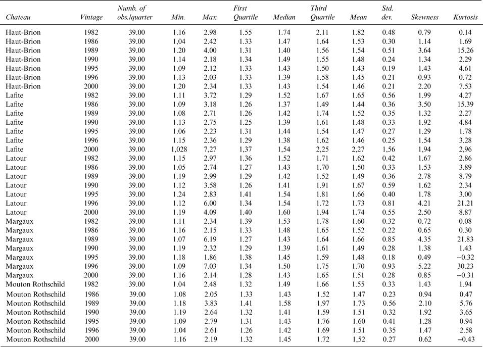
Appendix Tables A2 and A3 suggest the existence of strong price volatility for all auction houses and château-vintage pairs. Table A2 shows the average maximum and minimum price ratios within each auction over the entire period for each auction house and château-vintage pair. Column 1 in Table 2 exhibits an average value of the within indicator of 1.402, suggesting intra-auction price dispersions of more than 40 percent on average. Examining the wines in our sample and taking the mean value for all auction houses suggest that, with an average ratio of 1.14 (Table A2, last column), Mouton Rothschild 2000 exhibits the lowest average price volatility. In contrast, Lafite Rothschild 1982 displays the highest average price volatility, with an average ratio of 2.07.
Quarterly average maximum and minimum price ratios between auction houses for each châateau-vintage pair exhibit different spreads (Table A3). With the exception of Lafite Rothschild 2000 (with a mean ratio of 2.27) and the 1982 vintages, the means of ratios for almost all wines lie within a narrow interval [1.45; 1.55], which is significantly different from 1. These results confirm a high price volatility between (Table A3) and even within (Table A2) auction houses.
However, arbitrage strategies are profitable only if transaction costs are not prohibitively high. Therefore, we need to specify the arbitrage conditions to compare the ratios in Tables A2 and A3 with the arbitrage break-even point.
We define the break-even point value R and express it as a percentage of the château-vintage price. Denoting the price of the same châateau vintage in two different locations as j and j′, we can state the arbitrage profitability condition as follows:
![]() $P_B^j \; and\; P_S^{{j}^{\prime}} $
are the buyer price of the considered château vintage in the place j and the seller price of this château vintage in j′, respectively. This is the case when the arbitrage operation consists of buying in j and selling in j′ with
$P_B^j \; and\; P_S^{{j}^{\prime}} $
are the buyer price of the considered château vintage in the place j and the seller price of this château vintage in j′, respectively. This is the case when the arbitrage operation consists of buying in j and selling in j′ with
LT j , the local tax paid in j (expressed in %);
WE j , the wine-specific local tax (wine excise tax expressed in %);
![]() $TC_{jj^{\prime}}$
, the transport cost from j to j' (expressed in % of the buyer price in j in the case of twelve bottles per box transported by plane from Bordeaux to j');
$TC_{jj^{\prime}}$
, the transport cost from j to j' (expressed in % of the buyer price in j in the case of twelve bottles per box transported by plane from Bordeaux to j');
![]() $I_{jj{\prime}}$
, the insurance cost associated with transport (expressed in % of the buyer price in j); and
$I_{jj{\prime}}$
, the insurance cost associated with transport (expressed in % of the buyer price in j); and
![]() $T_{jj^{\prime}}$
, the tariff to enter j' country (expressed in % of the buyer price in j).
$T_{jj^{\prime}}$
, the tariff to enter j' country (expressed in % of the buyer price in j).
For simplicity, let us assume that
Because our database only provides buyer prices, we have to express the seller price
![]() $P_S^{{j}^{\prime}} $
as a function of the buyer price
$P_S^{{j}^{\prime}} $
as a function of the buyer price
![]() $P_B^{{j}^{\prime}} $
. Denoting
$P_B^{{j}^{\prime}} $
. Denoting
![]() $BP_{j^{\prime}}$
as the buyer premium of auction house j′ (expressed in %) yields
$BP_{j^{\prime}}$
as the buyer premium of auction house j′ (expressed in %) yields
![]() $P_B^{j^{\prime}} = P_S^{{j}^{\prime}} \left( {1 + BP_{{j}^{\prime}}} \right)$
.
$P_B^{j^{\prime}} = P_S^{{j}^{\prime}} \left( {1 + BP_{{j}^{\prime}}} \right)$
.
Thus, the arbitrage profitability condition can be rewritten as
 $P_A^{{j}^{\prime}} \gt R.P_A^j \; or\; \displaystyle{{P_A^{{j}^{\prime}}} \over {P_A^j}} \gt \; R$
, with
![]() $R = \left( {1 + X_{j{j}^{\prime}}} \right)\; \left( {1 + BP_{{j}^{\prime}}} \right)$
. Apparently, the value of R depends on j and j′. Table 4 offers calculations of R based on information on 2012 transaction costs shown in Table 3 (when the twelve-bottle case of wine is transported from Bordeaux to j′ by plane, i.e., in the most expensive way). Due to the rising buyer premiums over the last decade, 2012 exhibits the highest transaction costs.
$R = \left( {1 + X_{j{j}^{\prime}}} \right)\; \left( {1 + BP_{{j}^{\prime}}} \right)$
. Apparently, the value of R depends on j and j′. Table 4 offers calculations of R based on information on 2012 transaction costs shown in Table 3 (when the twelve-bottle case of wine is transported from Bordeaux to j′ by plane, i.e., in the most expensive way). Due to the rising buyer premiums over the last decade, 2012 exhibits the highest transaction costs.
Table 3 Transaction Costs on International Fine-Wine Auction Markets

a Significant lots are defined according to their scarcity, prestige, etc. The first five growths are all significant lots at the lowest confidence level (for very significant lots like the 1945 vintage, seller commission is 0 percent). Tariffs come from the World Trade Organization (http://tariffanalysis.wto.org/default.aspx); their value depends on the exporters' nationalities. Transport costs refer to Balguerie Transport (the biggest logistics firm in the Bordeaux wine trade).
Table 4 Transaction Cost (R) Calculation as % of Buyer Price in j in 2012

Calculation are based on data in Table 3. Auction Companies: ACM (Acker Merrall & Condit), HDH (Hart Davis Hart); Cities: NYC (New York City), HK (Hong Kong), LON (London), CHI (Chicago)
We can now compare the R-values provided in Table 4 with the maximum and minimum ratios of the between auction house prices reported in Appendix Table A3. If the ratios in Table A3 are larger than the values in Table 4, arbitrage opportunities may exist. According to Table 4, the maximum transaction cost is 1.566, and the average transaction cost is 1.363. Table A3 reports that the average maximum and minimum spread between two auction houses equals 1.571; the median of this maximum and minimum spread is 1.452. Both values are larger than the average transaction cost. Table A3 indicates that for some wines (e.g., Lafite Rothschild), the average maximum and minimum spread over the period is much larger than the average transaction cost of 1.363. Therefore, on average, the wine-auction market is characterized by a certain degree of price dispersion and offers some arbitrage opportunities.
IV. Hedonic Analysis
A. OLS Model
Hedonic functions relate the prices of differentiated goods to their attributes (e.g., Triplett, Reference Triplett2004). Wine prices are determined by such factors as appellation, vintage, expert opinion, reputation, and so forth. To control for time-invariant firm-specific characteristics, such as appellation, production techniques, and reputation, we also include château fixed effects. In addition, we add expert quality assessments (i.e., Parker points) for each château-vintage combination.
If LOOP holds, the location of the auction should be irrelevant, and marketplace or auction-house dummies should not be significant in a hedonic regression.
To increase the number of observations per time-unit we aggregate our quarterly data to annual data and run the following pooled model:
 $$\eqalign{ lnP_{it} =& \alpha _0 + \alpha _1Year_t + \alpha _2Age_{it} + \; \alpha _3Grade_{it} + \alpha _4Number_{it} + \alpha _5Case12 + \cr& \beta \mathop \sum \nolimits_{i = 1}^{65} Vintage_{it} + \gamma \mathop \sum \nolimits_{i = 1}^5 Chateau_i + \delta \mathop \sum \nolimits_{i = 1}^6 Country_{it} + \theta \mathop \sum \nolimits_{i = 1}^{14} City_{it} + \cr & \tau \mathop \sum \nolimits_{i = 1}^{13} Company_{it} + \; \varphi \mathop \sum \nolimits_{i = 1}^{33} Auction_{it} + \varepsilon _{it.}} $$
P it is the price of a château-vintage combination i sold at date t. α 0 is a constant, Vintage denotes vintage fixed effect, Year denotes year fixed effect, and Age controls for the wine's age at the date of sale; it is defined as Year-Vintage. Grade stands for critical scores (i.e., Parker points). Given the endogeneity of Parker points, Grade is only assumed to proxy a wine's quality and is not aimed at quantifying the price effect of Parker points. We assume a strong positive effect of Grade on a wine's price.
Number stands for the number of bottles per lot and tests the existence of price discounts for larger lots. However, even if there is a quantity discount, there might still be a premium for complete cases of twelve bottles, which, in the case of Bordeaux grand cru wines, are original wooden boxes, captured by the binary variable Case12. Against the background of rampant wine fraud (e.g., Hellman, Reference Hellman2017; Wallace, Reference Wallace2008),Footnote 7 particularly on the Bordeaux grand cru market, we hypothesize that lots with complete cases may lend some credibility toward the wine's authenticity and therefore demand a premium. In addition, a complete case of twelve bottles in a wooden box may also have a trophy value. We complete the equation with the inclusion of various additional fixed effects for Château, auction Company, auction City, and the specific Auction (which is the combination of Company and City, e.g., Christie's New York or Christie's Hong Kong).
Tables 5a and 5b display the hedonic regression results of five variants of equation (5). In column 1 of Table 5a, we report the results for equation (5) without any Country, City, Company, and Auction fixed effects. We find significantly positive effects of Age, Grade, and Case12 on the price. The marginal age effect of approximately 8.3 percent, which denotes the nominal rate of return to holding Bordeaux grand cru wine, appears high compared to past analyses. However, note that our study period is between 2001 and 2012, which includes the peak of the fine-wine pricing curve. The quantity discount of about 0.3 percent per additional bottle in the lot appears to be very small (although statistically significant), the full case premium of approximately 9.5 percent across all wines and auctions more than offsets the quantity discount.
Table 5a Hedonic Model for Auction Prices, 2000–2012
Country, City, and Company Dummies; Dependent Variable ln(price)
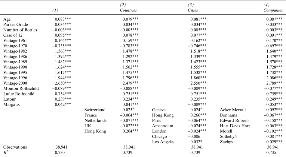
The reference variables for the dummy variables are 1959 (vintage), Haut Brion (wine), Christie's (company), New York (city), and United States (country); all equations contain an intercept and year fixed effects (not reported here). Significance levels 1% (***), 2% (**), 5% (*), and 10% (+) are based on robust standard errors.
Table 5b Hedonic Model for Auction Prices, 2000–2012
Auction Dummies; Dependent Variable ln(price)
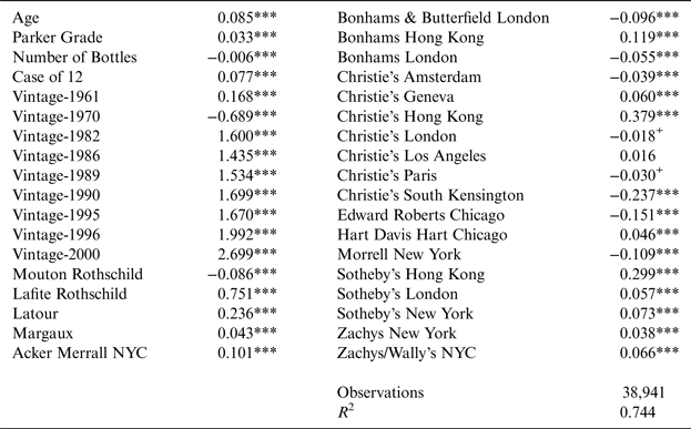
The reference variables for the dummy variables are 1959 (vintage) Haut Brion (wine), and Christie's New York (auction); all equations contain an intercept and year fixed effects (not reported here). Significance levels 1% (***), 2% (**), 5% (*), and 10% (+) are based on robust standard errors.
We further notice substantial vintage effects that appear to favor recent over past vintages. In addition, compared to the reference Haut-Brion, our results suggest the existence of a 75 percent premium for Château Lafite Rothschild, even after controlling for quality.
Columns 2, 3, and 4 of Table 5a as well as Table 5b display variants of this base model. Alternating, we add fixed affects for Countries, Cities, auction Companies, and specific Auctions. Overall, the coefficient of the basic appear to remain fairly robust across all variants. However, we do find significant differences between auction locations. When we add country dummies (Table 5a, column 2), we find statistically significant but small discounts compared to the reference country (i.e., the United States), in the Netherlands (–7.1 percent), France (–6.4 percent) and the United Kingdom (–2.2 percent). In contrast, China demands a surcharge of 26.4 percent. This pattern remains unchanged in all other variants. Prices at most European auctions are below the U.S. levels, but prices in Hong Kong are substantially higher. For instance, Christie's Hong Kong prices are approximately 37.9 percent above those of Christie's New York.
B. Quantile Regression Model
To analyze regional price differences and the respective marginal effects of certain wine attributes, we run interacted variables. Our model is similar to the one described in column 2 of Table 5a (i.e., we employ country dummy variables).
There are only two distinctions to the model shown in Table 5a. First, to detect possible regional differences, we interact the variables Age, Points, Case12, and Lafite Rothschild with all country dummy variables (i.e., Switzerland, France, the Netherlands, the United Kingdom, and Hong Kong). The United States is not interacted and serves as reference. The coefficients for the interactions indicate whether the respective variable's price impact is significantly different from the reference.
Second, and in contrast to equation (5), we also test the hypothesis that wine buyers in Hong Kong are less concerned about counterfeit wines and do not demand discounts for suspicious bottles. We generate a new variable called GoogleFake that draws on data from Google Trends. For each wine-vintage combination, we track the term “fake wine” and its translations into French (faux vin) and Chinese (假洋酒) and count the mentions over time. Table 6 reports the 2005 and 2012 GoogleFake values for various château-vintage combinations. GoogleFake values tend to grow over time but vary significantly among châteaux and vintages, resulting in a range of 0 to 533.Footnote 8 A first glimpse, provided in Table 6, suggests that 1986 is a low GoogleFake value vintage and that Haut-Brion exhibits fewer mentions than its competitors. In contrast, Mouton Rothschild, Lafite, and some Latour wines receive more Google mentions.
Table 6 GoogleFake Mentions of Selected Wines in 2005 and 2012
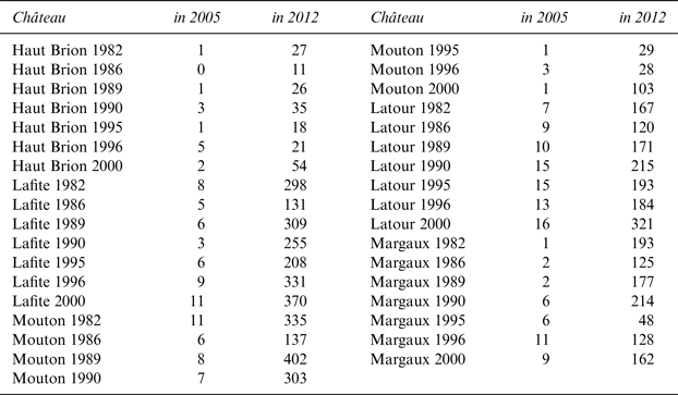
We hypothesize that GoogleFake mentions reflect “chatter” in the wine community; a high GoogleFake value for “fake wine,” therefore, displays higher awareness (and a higher counterfeit probability for this wine).
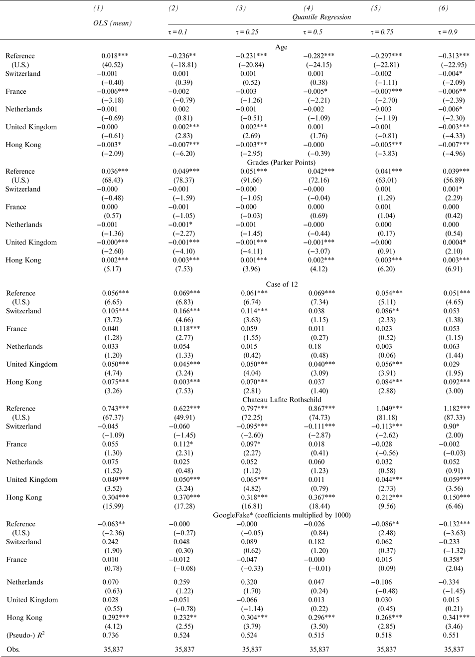
Due to the high degree of skewness in our price data (see also Table 1) and potentially varying marginal effect in different price brackets, we run various quantile regressions. The results are reported in Table 7, where columns 2 to 6 show the effects for the quantiles τ = 0.1, 0.25, 0.5, 0.75, and 0.9. For the sake of comparison, we report the corresponding ordinary least squares (OLS) coefficients in column 1.
Table 7 Quantile Regressions of Country Interactions with Age, Grades, Case12, and Lafite-Rothschild
Dependent Variable ln(price)

All equations include a constant term and a control variable for number of bottles per lot and dummy variables for vintage, year of sale, and château. The United States is the reference for all non-interacted terms. Significance levels are 1% (***), 2% (**), and 5% (*), respectively.
First, in contrast to the OLS results reported in column 1, the Age variable exerts a negative effect on prices; the price discount appears to increase in higher price brackets. Hong Kong exhibits a slightly more pronounced negative price effect in all quantiles.
Second, similar to the OLS results, wine prices are positively affected by Parker scores. However, the effect peaks in the 25 percent quantiles and decreases thereafter. Again, Hong Kong's Parker-score effects are statistically significantly stronger in every quantile, although at minimal levels.
Third, although the Case12 variable has a significantly positive effect in all markets, its effect in Hong Kong is more than twice as high as in the reference (i.e., the United States); this result is true for almost all price quantiles. We observe similar positive deviations from the reference in Switzerland and in the United Kingdom.
Fourth, like the OLS regression, the quantile regression shows Lafite effects that increase with the price quantiles. For the references, the Lafite coefficient grows from 0.622 for τ = 0.1 to 1.182 for τ = 0.9. Hong Kong exhibits significantly stronger Lafite effects, especially within the lower quantiles. For instance, Hong Kong's Lafite effect equals 0.992 (i.e., 0.622 + 0.370) in quantile τ = 0.1 and 1.332 (i.e., 1.182 + 0.150) in quantile τ = 0.9. Other than Hong Kong, only the United Kingdom shows a Lafite effect that is significantly higher than the reference.
Fifth, the GoogleFake variable seems to exert a negative price effect only in the highest price quantile and remains insignificant for less-expensive wines on almost all markets. However, Hong Kong's wine prices display strong positive deviations from the reference. Not only are the deviations significant at the 1-percent level in all quantiles; their size more than offsets the negative reference effect. For instance, the GoogleFake coefficient for the reference (i.e., the United States) equals –0.132, but it is + 0.209 (i.e., –0.132 + 0.341) in Hong Kong. Counterfeit suspect wines are less expensive on most markets, yet they fetch a premium in Hong Kong. Whether this difference is due to a higher status value of certain wines or less experience, as claimed in the documentary Red Obsession (Roach and Ross, Reference Roach and Ross2013), we cannot answer.
Overall, the wine-auction market in Hong Kong is significantly different from most other established auction markets in several ways. Hong Kong buyers seem to prefer younger wines that are highly critically acclaimed and sold in full cases of twelve. They are also willing to pay a higher premium for Château Lafite Rothschild wines and, interestingly, for wines that are deemed counterfeit suspects on the Internet.
V. Conclusion
We analyze a large set of fine-wine prices from numerous auctions held between 2000 and 2012 in six countries. We find that the price ranges for most wines far exceed transaction costs, suggesting the existence of substantial price dispersion, which is only partially explained by the heterogeneity of some sales. A hedonic analysis suggests that auction prices in Hong Kong are significantly higher than in the other locations, such as New York, London, or Paris.
We find that wine prices in Hong Kong auctions are substantially more sensitive to certain wine characteristics than in other established auction markets. In particular, young wines with high critical scores attain higher prices than elsewhere. In addition, there are higher premiums for sales of full cases of twelve bottles and for wines by Château Lafite Rothschild, indicating some orientation toward prestige wines. Our results also suggest the existence of a price premium for wines that are deemed counterfeit suspects on the Internet and sell at discounted prices in Europe and the United States.
Nevertheless, our results suffer from several limitations.
First, the possibility that seemingly identical lots may, in fact, be heterogeneous suggests the inclusion of additional variables, such as ullage, quality of label, cork, and capsule.
Second, when comparing price ranges and transaction costs in Section III, we use average quarterly prices instead of contemporaneous prices. Due to the illiquidity of the fine-wine market, perfectly contemporaneous prices are virtually unavailable. Simultaneous wine auctions where an arbitrageur could simultaneously (by phone or Internet) buy in one auction house and sell in another are virtually nonexistent. Due to the time differences between auctions, our test of the strong version of LOOP is not conclusive.
Third, our analysis only focuses on the strong version of LOOP. We have not analyzed its weak form (i.e., any systematic price convergence of certain wines sold at different locations).
In fact, it is not a priori clear whether some arbitrage has been happening and the weak form of LOOP applies. In future research, one may examine whether wines that are particularly appreciated in Hong Kong (i.e., highly rated, counterfeit-suspect cases of Lafite) have been systematically moved from Europe and the United States to China. The burst of the Lafite bubble and the following retreat of fine-wine prices in Hong Kong and later Shanghai may be an indication of some ongoing arbitrage (Roach and Ross, Reference Roach and Ross2013).
Appendix
Table A1 Breakdown of Transactions by Vintages

Table A2 Means of Maximum/Minimum Price Ratios within Individual Auctions
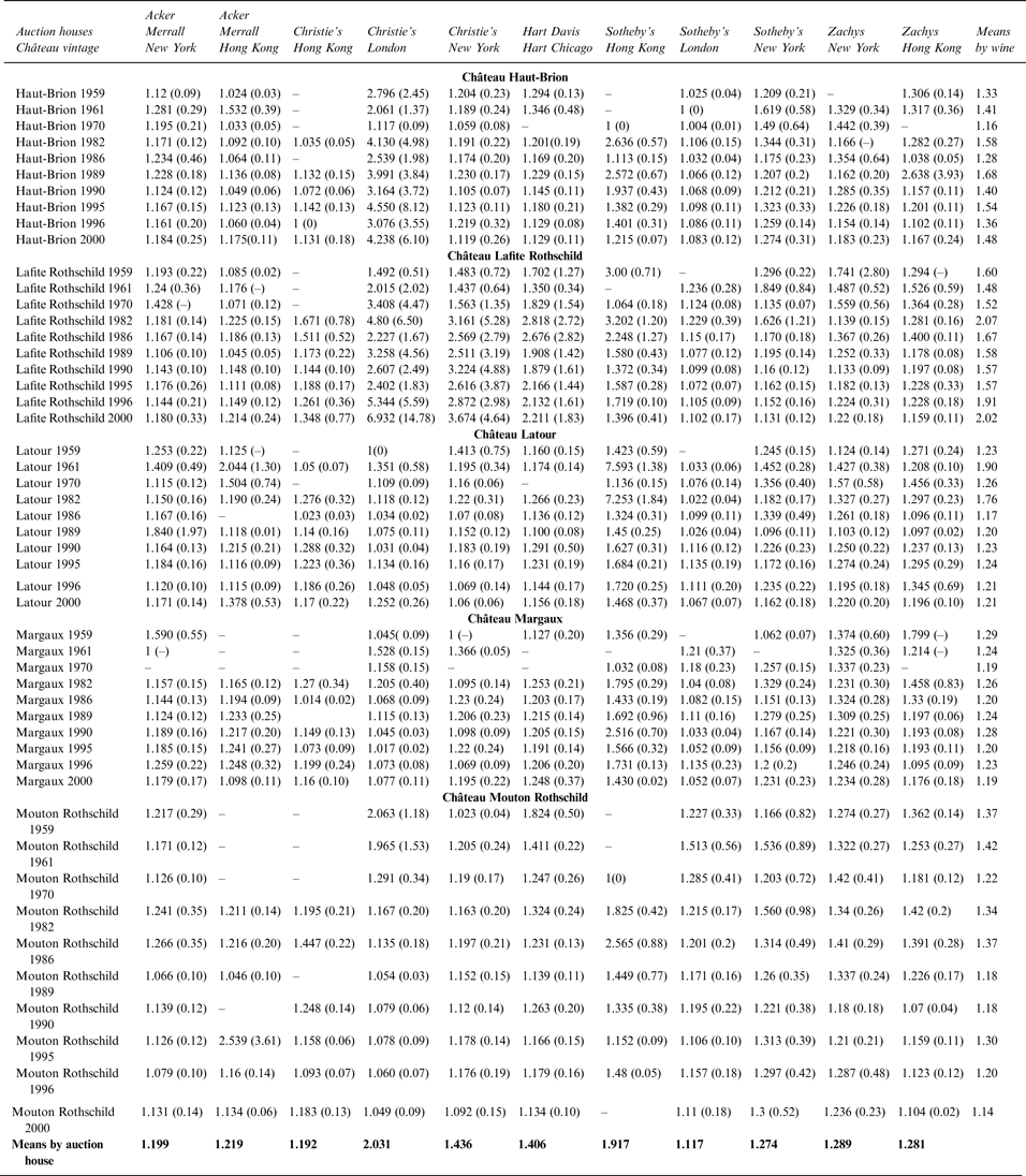
Table A3 Means of Quarterly Maximum/Minimum Price Ratios between Auction Houses


