


1. Introduction
Free-surface turbulence is a ubiquitous phenomenon encountered in very diverse natural systems, such as rivers, lakes, oceans, etc. The presence of the free surface affects the underlying turbulence by both dynamic and kinematic boundary conditions (Shen et al. Reference Shen, Zhang, Yue and Triantafyllou1999). The former requires zero tangential stresses at the free surface and produces the surface layer, which is a thin region adjacent to the free surface characterized by fast variations of horizontal vorticity components. The latter requires no vertical mass flux passing through the free surface and produces the blockage (or ‘source’) layer with a thickness of the order of the macroscale/outer lengthscale (for the open channel flows considered in this study, the macroscale/outer length scale corresponds to the water depth).
The two boundary conditions introduce some unique turbulence features near the free surface. One well-known phenomenon is the redistribution of turbulent kinetic energy (TKE) in the blockage layer, namely the increase of horizontal velocity fluctuations at the expense of reduction of the vertical component, which has been reported in different flows with a free surface (Nezu & Rodi Reference Nezu and Rodi1986; Handler et al. Reference Handler, Swean, Leighton and Swearingen1993; Pan & Banerjee Reference Pan and Banerjee1995; Nagaosa Reference Nagaosa1999; Shen et al. Reference Shen, Zhang, Yue and Triantafyllou1999; Lee et al. Reference Lee, Suh, Sung and Pettersen2012; Zhong et al. Reference Zhong, Li, Chen and Wang2015).
Owing to the fact that velocity fluctuations result from the passing and evolution of turbulence structures, the TKE redistribution phenomenon indicates that turbulence structure features in the near-free-surface region of these free-surface turbulence flows (e.g. the open channel flow (OCF) considered herein) are different from those at equivalent positions in other wall flows without a free surface (e.g. turbulent boundary layer (TBL), pipe flow and closed channel flow (CCF)). Perot & Moin (Reference Perot and Moin1995) and Walker, Leighton & Garza-rios (Reference Walker, Leighton and Garza-Rios1996) reported that the horizontal parts of vortex filaments induce splat and anti-splat events at the free surface when they approach the free surface. These splat and anti-splat events play decisive roles on the TKE redistribution in OCFs via the pressure–strain effect (Nagaosa Reference Nagaosa1999). The reduction of vertical length scales and increase of horizontal length scales in the near-free-surface region of OCFs make vortex filaments more pancake-like structures (Handler et al. Reference Handler, Swean, Leighton and Swearingen1993). It has been demonstrated that the horizontal parts of vortex filaments are dissipated quickly near the free surface, while the quasi-vertical parts connected to the free surface are persistent and decay slowly (Pan & Banerjee Reference Pan and Banerjee1995; Nagaosa Reference Nagaosa1999; Shen et al. Reference Shen, Zhang, Yue and Triantafyllou1999; Nagaosa & Handler Reference Nagaosa and Handler2003).
Some recent studies further revealed differences of large turbulence structures in OCFs when compared to other wall flows. For instance, Peruzzi et al. (Reference Peruzzi, Poggi, Ridolfi and Manes2020) showed that the large-scale and very-large-scale motions (LSMs and VLSMs) are detectable over a much larger wall-normal extent in OCFs, and VLSMs can appear at friction Reynolds number  $Re_\tau$ as low as 725, which is much lower than that normally required in other wall flows. Duan et al. (Reference Duan, Chen, Li and Zhong2020) demonstrated that the strength of VLSMs in OCFs is higher than that in other wall flows. And this strength difference of VLSMs is closely related to the phenomenon of TKE redistribution, i.e. the higher streamwise turbulence intensity in the near-free-surface region of OCFs is mainly contributed by the higher strength of VLSMs therein.
Though these studies have promoted our understandings of unique turbulence structures in the near-free-surface region of OCFs, most of them mainly focused on the turbulence structure statistics of geometrical shapes, length scales, strengths/intensities, etc. Besides these features, another feature that is significant is population densities. However, the question of how the free surface would affect the population densities of turbulence structures remains open.
To fill this gap, the population densities of spanwise vortices in smooth-walled OCFs were investigated in this paper. Instead of rough-walled OCFs, smooth-walled OCFs were considered to ensure that the only difference between OCFs and other wall flows (such as CCFs and TBLs) is the outer boundary condition. Then comparisons between OCFs and other wall flows are possible and the resulting difference would directly reflect the unique outer boundary effect of the free surface on the population characteristics of spanwise vortices in OCFs.
2. Datasets and methodology
Throughout this paper, the streamwise, wall-normal and spanwise directions are denoted by  $x$,
$x$,  $y$ and
  $z$, respectively. For the wall-normal coordinate, the location
  $y=0$ is right at the wall. The mean velocities along
  $x$,
$x$,  $y$ and
  $z$ directions are denoted as
  $U$,
$U$,  $V$ and
  $W$, with corresponding fluctuating velocities denoted as
  $u$,
$u$,  $v$ and
  $w$, respectively. The root mean square is denoted by a prime and ensemble average is indicated by
  $\langle {~}\rangle$. The superscript ‘
 $^{+}$’ denotes an inner-scale normalization using kinematic viscosity
  $\nu$ and friction velocity
  $u_\tau$, e.g.
  $U^{+}=U/u_\tau$,
  $y^{+}=y/l_*$ (where
  $l_*=\nu /u_\tau$ is the inner length scale), etc. For the convenience of descriptions,
  $h$ will be used to generally refer to the water depth of OCF, the channel half height of CCF and the boundary layer thickness of TBL. The definition of the friction Reynolds number
  $Re_\tau$ for all the three flow scenarios (OCF, CCF and TBL) is
  $Re_\tau =u_\tau h/\nu$.
2.1. Open channel flow datasets
Four experimental and numerical OCF cases were considered in this study, with the friction Reynolds number  $Re_\tau$ ranging from 950 to 2407 (see table 1). The first three experimental OCF cases (
 $Re_\tau =1030$, 1903 and 2407, hereafter denoted as OCF1030, OCF1903 and OCF2407) correspond to the flow cases in the authors’ previous study (Duan et al. Reference Duan, Chen, Li and Zhong2020), among which the experiment of the OCF1030 case was performed in a 20 m long and 0.3 m wide flume, while the experiments of the OCF1903 and OCF2407 cases were conducted in a longer and wider flume (31 m long and 0.56 m wide). The friction velocity
  $u_\tau$ in all three cases was determined by fitting the mean velocity profile with the log law
  $U^{+}=({1}/{\kappa })\ln (y^{+})+A$ (with
  $\kappa =0.412$ and
  $A=5.29)$ (Nezu & Nakagawa Reference Nezu and Nakagawa1993). The channel slope
  $S$ values for the OCF1030, OCF1903 and OCF2407 cases are 0.002, 0.0018 and 0.0018, respectively, and the uncertainties of
  $S$ are estimated to be less than 2.5 % of
  $S$. In all cases, the aspect ratio
  $B/h$ (with
  $B$ the channel width and
  $h$ the water depth) is greater than 7.2, which is large enough to ensure two-dimensional (2-D) flow conditions in the central region of the flow according to the classical threshold of 5 (Nezu & Nakagawa Reference Nezu and Nakagawa1993; Nezu Reference Nezu2005). The water depth
  $h$ was measured by ultrasonic level sensors with measurement uncertainty of 0.2 mm.
Table 1. A summary of the open channel flow (OCF), closed channel flow (CCF) and turbulent boundary layer (TBL) datasets:  $Re_\tau$, friction Reynolds number;
  $B$, channel width;
  $h$, water depth/channel half height/boundary layer thickness;
  $U_\infty$, free-surface velocity/channel centreline velocity/boundary layer free-stream velocity;
  $L_x$,
  $L_y$ and
  $L_z$, velocity field dimensions along streamwise, wall-normal and spanwise directions;
  $\Delta x^{+}$,
  $\Delta y^{+}$ and
  $\Delta z^{+}$, inner-scale normalized velocity vector spacings along corresponding directions; and
  $N_{F3D}$ in numerical cases, the number of three-dimensional (3-D) velocity fields.

The velocity measurement section was located 12 m and 16.5 m downstream of the flume entrance in the short and long flumes, respectively. The distances (greater than  $210h$) are sufficiently long – much longer than the criterion of
  $76h$ Kirkgöz & Ardiçliolu (Reference Kirkgöz and Ardiçliolu1997) – to ensure that the flow is fully developed at the measurement location. The 2-D particle image velocimetry (PIV) measurements were performed in a streamwise–wall-normal (
 $xy$) plane at the channel spanwise centre to obtain velocity fields. The measurement plane was illuminated by a 1.5 mm thick laser sheet and a high-speed complementary metal oxide semiconductor (CMOS) camera (
 $1920 \times 1080$ pixels) was used for the particle image acquisition. Hollow glass spheres with a density of
  $1.06\times 10^{3}\ \textrm {kg}\ \textrm {m}^{-3}$ and mean diameter of
  $10\ \mathrm {\mu }\textrm {m}$ were used as tracer particles.
For each of the three experimental flow cases, two kinds of PIV velocity fields were obtained. The first is a time-resolved velocity field with a small field of view (FOV; streamwise  $\times$ wall-normal velocity field dimension
  $L_x\times L_y = 0.09h\times h$), and this kind of velocity field was adopted in Duan et al. (Reference Duan, Chen, Li and Zhong2020) for the spectrum analysis of the characteristics of VLSMs in OCFs. The second is independent velocity fields with larger FOV (
 $L_x\times L_y=0.8h\times h$), which was adopted in this study for investigating the characteristics of spanwise vortices. For each flow case, 4999 independent particle image pairs (corresponding to 4999 independent velocity fields) were acquired to allow statistical quantifications. The particle images were post-processed in an in-house PIV software using a multi-pass and multi-grid window deformation method (similar to that of Scarano Reference Scarano2002) to get velocity fields. The interrogation window sizes were adjusted case by case to obtain similar inner-scale normalized vector spacings (
 $\Delta x^{+} = \Delta y^{+} =10.8 - 13.9$) due to the fact that spanwise vortices can be scaled by the inner length scale (Carlier & Stanislas Reference Carlier and Stanislas2005; Chen et al. Reference Chen, Adrian, Zhong, Li and Wang2014).
Based on the consideration that the above independent velocity field data have not been presented in Duan et al. (Reference Duan, Chen, Li and Zhong2020), the data accuracy needs to be discussed herein for completeness and such data accuracy verification is presented in the Appendix by showing typical turbulence statistics as well as the uncertainties.
In addition to the three experimental OCF cases, one direct numerical simulation (DNS) OCF case ( $Re_\tau =950$, denoted as OCFDNS950) from Wang & Richter (Reference Wang and Richter2019) (see case 8 therein) was further considered. The 3-D velocity field dimension (streamwise
  $\times$ wall-normal
  $\times$ spanwise) is
  $L_x\times L_y \times L_z = 10.8h\times h \times {\rm \pi}h$. The original inner-scale normalized vector spacing
  $\Delta x_o^{+}\times \Delta y_o^{+}\times \Delta z_o^{+}$ is
  $10\times (1, 6.4)\times 5.8$. Here the two values of
  $\Delta y_o^{+}$ correspond to the vector spacing at the wall and outer boundary, respectively. Streamwise–wall-normal and spanwise–wall-normal planes (i.e.
  $xy$ and
  $yz$ planes) were extracted from the 3-D velocity fields to investigate spanwise vortices and streamwise vortices, respectively (the reasons for investigating streamwise vortices will be explained in § 3.3). Successive planes were separated by a distance roughly equal to
  $100l_*$ and
  $500l_*$ for
  $xy$ planes and
  $yz$ planes, respectively. The number of 3-D velocity fields
  $N_{F3D}$ is 48, based on which 1488
  $xy$ planes and 1008
  $yz$ planes were obtained. Following Herpin, Stanislas & Soria (Reference Herpin, Stanislas and Soria2010), to avoid the effect of non-uniform wall-normal velocity spacing on vortex identifications, the extracted
  $xy$ and
  $yz$ planes were interpolated on a regular mesh using 2-D bicubic spline interpolations. The final inner-scale normalized vector spacing in the
  $xy$ plane is
  $\Delta x^{+}=\Delta y^{+}=\Delta x_o^{+}$, while the vector spacing in the
  $yz$ plane is
  $\Delta y^{+}=\Delta z^{+}=\Delta z_o^{+}$.
2.2. Closed channel flow and turbulent boundary layer datasets for comparison
For comparison purposes, six experimental and numerical CCF and TBL cases at comparable Reynolds numbers with that of OCF cases were considered (as summarized in table 1). The first four experimental CCF and TBL cases (CCF1185, CCF1760, TBL1400 and TBL2350) are from Wu & Christensen (Reference Wu and Christensen2006). As that in experimental OCF cases, similar  $xy$ plane 2-D PIV measurements were performed in these CCF and TBL cases (see table 1 for detailed parameters). Owing to the lack of raw velocity field data, all the vortex results of the four CCF and TBL cases shown in this study were based on the results presented in Wu & Christensen (Reference Wu and Christensen2006).
The last two CCF and TBL DNS cases – CCFDNS934 with  $Re_\tau =934$ (del Álamo et al. Reference del Álamo, Jiménez, Zandonade and Moser2004) and TBLDNS1000 with
  $Re_\tau =1000$ (Sillero et al. Reference Sillero, Jiménez and Moser2013) – were adopted mainly for comparison with the OCF DNS case at comparable Reynolds number (i.e. OCFDNS950 case). The raw 3-D velocity fields can be freely accessed from https://torroja.dmt.upm.es/turbdata/. For the CCFDNS934 case, the 3-D velocity field dimension
  $L_x\times L_y \times L_z = 8{\rm \pi} h\times 2h \times 3{\rm \pi} h$ (only the bottom half of the full channel was considered herein). For the TBLDNS1000 case, the velocity fields were extracted from the raw TBL DNS velocity fields of the
  $BL_{6600}$ case in Sillero et al. (Reference Sillero, Jiménez and Moser2013) (
 $Re_\tau$ ranges from 981 to 2025 as the boundary layer develops along the streamwise direction) at a streamwise location where
  $Re_\tau$ equals 1000. The extracted 3-D velocity field dimension
  $L_x\times L_y \times L_z$ of the TBLDNS1000 case is
  $2h\times h \times 16h$. Here the streamwise dimension
  $L_x$ is chosen to be
  $2h$ to ensure that
  $Re_\tau$ is not much different from 1000 (
 $Re_\tau =988 - 1011$). Similar to the OCFDNS950 case,
  $xy$ planes and
  $yz$ planes were extracted from the 3-D velocity fields of CCFDNS934 and TBLDNS1000 cases and interpolated on regular meshes. The vector spacings were chosen to be identical to that of OCFDNS950 cases to allow comparisons, i.e.
  $\Delta x^{+}=\Delta y^{+}=10$ in the
  $xy$ plane, while
  $\Delta y^{+}=\Delta z^{+}=5.8$ in the
  $yz$ plane. Detailed parameters for these extracted planes are summarized in table 1 and will not be discussed herein for brevity.
2.3. Vortex identification method
The same  $\lambda _{ci}$-criterion-based vortex identification method as in Wu & Christensen (Reference Wu and Christensen2006) was employed to facilitate comparisons. The method utilizes the imaginary part of the complex eigenvalue of the local velocity gradient tensor, namely the swirling strength
  $\lambda _{ci}$, to identify vortices. Given that
  $\lambda _{ci}$ does not yield the sense of rotation direction, a signed swirling strength
  $\varLambda _{ci}$ was adopted. Taking the identification of spanwise vortices in the
  $xy$ plane as an example,
  $\varLambda _{ci}(x,y)$ can be defined as
 \begin{equation} \varLambda_{ci} (x, y)=\lambda_{ci} (x, y)\dfrac{\omega_z(x, y)}{|\omega_z(x, y)|}, \end{equation}
where  $\omega _z$ is the instantaneous fluctuating spanwise vorticity. Then a normalized form of
  $\varLambda _{ci}(x,y)$,
 \begin{equation} \tilde{\varLambda}_{ci}(x, y)=\dfrac{\varLambda_{ci} (x, y)}{\varLambda_{ci}^{\prime} (y)}, \end{equation}
was taken as a basis for defining a universal threshold for vortex identifications. Following Wu & Christensen (Reference Wu and Christensen2006), the same universal threshold of  $|\tilde {\varLambda }_{ci}(x,y)|=1.5$ was adopted. Then regions with at least three points satisfying
  $|\tilde {\varLambda }_{ci}(x,y)|\geqslant 1.5$ in both
  $x$ and
  $y$ directions were identified as spanwise vortices, among which regions with
  $\tilde {\varLambda }_{ci}(x,y)\geqslant$1.5 and
  $\tilde {\varLambda }_{ci}(x,y)\leqslant -1.5$ correspond to retrograde and prograde ones, respectively.
For the identification of streamwise vortices in the  $yz$ plane, the procedures are similar, and
  $\varLambda _{ci}$ and
  $\tilde {\varLambda }_{ci}$ can be given by
 \begin{equation}
\left.\begin{aligned} \varLambda_{ci} (z,
y)=\lambda_{ci} (z, y)\dfrac{\omega_x(z, y)}{|\omega_x(z,
y)|}, \\ \tilde{\varLambda}_{ci}(z,
y)=\dfrac{\varLambda_{ci} (z, y)}{\varLambda_{ci}^{\prime}
(y)}, \end{aligned}\right\} \end{equation}
\begin{equation}
\left.\begin{aligned} \varLambda_{ci} (z,
y)=\lambda_{ci} (z, y)\dfrac{\omega_x(z, y)}{|\omega_x(z,
y)|}, \\ \tilde{\varLambda}_{ci}(z,
y)=\dfrac{\varLambda_{ci} (z, y)}{\varLambda_{ci}^{\prime}
(y)}, \end{aligned}\right\} \end{equation}
with  $\omega _x$ denoting the instantaneous fluctuating streamwise vorticity. Then the regions with at least three points satisfying
  $|\tilde {\varLambda }_{ci}(z,y)|\geqslant 1.5$ in both
  $z$ and
  $y$ directions were identified as streamwise vortices. It is worth mentioning here that streamwise vortices are analysed only in § 3.3 and thus all vortices discussed elsewhere refer to spanwise vortices.
3. Results and discussions
3.1. Population trends of spanwise vortices
The population density of prograde (or retrograde) vortices  $\varPi _p(y)$ (or
  $\varPi _r(y)$) can be quantified once individual spanwise vortices are extracted. Following Wu & Christensen (Reference Wu and Christensen2006),
  $\varPi _{p(r)}(y)$ is defined as the ensemble-averaged number of prograde (retrograde) spanwise vortices,
  $N_{p(r)}(y)$, whose centres reside in a non-dimensional rectangular area of wall-normal height
  $3\Delta y/h$ and streamwise extent
  $L_x/h$ centred at
  $y$. Here a wall-normal height of
  $3\Delta y/h$ is used to decrease the profile scatter. Hence,
  $\varPi _{p(r)}(y)$ is given as
 \begin{equation} \varPi_{p(r)}(y)=\frac{N_{p(r)}(y)}{\,\dfrac{3\Delta y}{h} \dfrac{L_x}{h}\,}=\frac{N_{p(r)}(y)}{3\Delta y L_x}h^{2}. \end{equation}
 Similar to other wall flows, both prograde and retrograde vortex population densities in OCFs show a  $Re_\tau$ dependence as
  $\varPi _{p(r)}\propto Re_\tau ^{n}$. Wu & Christensen (Reference Wu and Christensen2006) reported
  $\varPi _{p}\sim Re_\tau ^{1.17}$ and
  $\varPi _{r}\sim Re_\tau ^{1.5}$ in TBLs and CCFs. The present four OCF cases yield
  $\varPi _{p}\sim Re_\tau ^{1.25}$ and
  $\varPi _{r}\sim Re_\tau ^{1.51}$, as shown in figure 1(a) and 1(b), respectively. Error bars are also presented to show the uncertainties. The almost invisible error bars indicate that the uncertainties are negligible. Therefore, error bars are no longer shown in the following figures unless it is necessary. Retrograde vortices exhibit a higher
  $n$ in all flow types, indicating that they are more sensitive to Reynolds number.

Figure 1. Reynolds-number scaling of the population of spanwise vortices in OCFs: ( $a$)
$a$)  $\varPi _{p}\sim Re_\tau ^{1.25}$ and (
 $b$)
$b$)  $\varPi _{r}\sim Re_\tau ^{1.51}$. Error bars are included to show the uncertainty.
3.2. Additional spanwise vortices in open channel flows
Comparisons of the population densities of spanwise vortices among different flow types (OCFs, TBLs and CCFs) will be performed to reveal the phenomenon of additional spanwise vortices in OCFs.
Given the fact that many factors (such as spatial resolution, noise level and processing procedures of the velocity fields) will directly affect the number of identified vortices, the vortex population density  $\varPi _{p(r)}$ values obtained from different data sources generally do not allow direct comparisons. In this study, the vortex population density
  $\varPi _{p(r)}$ is normalized by the value at
  $y/h=0.2$ to facilitate comparisons among different flow types:
 \begin{equation} {\rm \pi}_{p(r)}(y/h)=\dfrac{\varPi_{p(r)}(y/h)}{\overline{\varPi_{p(r),0.2}}},\quad \overline{\varPi_{p(r),0.2}}=10 \int_{y/h=0.15}^{y/h=0.25}\varPi_{p(r)}(y/h) \,\mathrm{d}(y/h). \end{equation}
 Figure 2 compares the  ${\rm \pi} _{p(r)}$ profiles for different flow types (OCFs, TBLs and CCFs). It can be seen from figure 2(a) that
  ${\rm \pi} _p$ displays a monotonic decrease in the entire flow for all flow types (except the OCFDNS950 case, where a dramatic increase appears in the near-free-surface region
  $y/h>0.95$; this phenomenon will be explained later). The decreasing trend of
  ${\rm \pi} _p$ is understandable since most vortices are generated near the wall and they continue to dissipate and merge with each other when they grow away from the wall. The three flows produce very similar
  ${\rm \pi} _p$ in the region
  $y/h<0.2$, which is also unsurprising because the same factors, no-slip boundary condition and viscosity, dominate this region in all three flow types. Beyond
  $y/h=0.2$, however, the results from different flow types gradually separate. Comparisons of the experimental results of the three flow types reveal the highest
  ${\rm \pi} _p$ in OCFs compared to TBLs and CCFs (especially in the near-free-surface region, e.g.
  $y/h>0.9$).

Figure 2. Comparison of the normalized vortex population density  ${\rm \pi} _{p(r)}$ among different flow types: (
 $a$)
$a$)  ${\rm \pi} _p$ and (
 $b$)
$b$)  ${\rm \pi} _r$. Lines and symbols are used to distinguish DNS and experimental cases.
Comparisons of the DNS results of the three flow types at  $Re_\tau \approx 1000$ (i.e. OCFDNS950, TBLDNS1000 and CCFDNS934 cases) indicate that
  ${\rm \pi} _p$ in TBL can be higher than that of OCF and CCF cases below
  $y/h=0.8$. While in the region
  $y/h>0.95$,
  ${\rm \pi} _p$ in the OCF DNS case exhibits a dramatic increase and tends to be significantly higher than that in TBL and CCF DNS cases. The difference between the experimental and DNS results may be caused by the boundary condition difference between experiments and DNS. For instance, the OCF DNS case used a rigid and free-slip boundary condition to model the free surface, which is somewhat different from the freely fluctuating free surface in experiments. The free-surface fluctuations in experiments could lead to a wider redistribution of the spanwise vortices and thus the dramatically increasing trend of
  ${\rm \pi} _p$ in the OCF DNS case is flattened in the experimental OCF cases. This speculation is well supported by the more flat
  ${\rm \pi} _p$ profiles in experimental OCF cases compared to that in the OCFDNS950 case. Even though the experimental and DNS results exhibit differences, both of them demonstrate that
  ${\rm \pi} _p$ in OCFs is higher than that in TBLs and CCFs, at least in the near-free-surface region.
Now let us focus on retrograde vortices (i.e.  ${\rm \pi} _r$, see figure 2b). In the region
  $y/h\lesssim 0.2$,
  ${\rm \pi} _r$ in all three flows monotonically increases. This can be explained by the variation of mean shear, i.e. the strong mean shear near the wall suppresses the development of retrograde vortices, while, moving away from the wall, the mean shear declines rapidly, based on which more retrograde vortices can be observed. Beyond
  $y/h\approx 0.2$,
  ${\rm \pi} _r$ shows totally different trends and magnitudes in different flows. In TBLs
  ${\rm \pi} _r$ reaches its maximum at
  $y/h\approx 0.2$ and then continuously decreases, while in experimental OCF cases
  ${\rm \pi} _r$ shows no obvious decreases and maintains a higher magnitude throughout the region
  $y/h>0.2$. Even for the OCF DNS case (OCFDNS950 case),
  ${\rm \pi} _r$ also only slightly decreases beyond
  $y/h=0.2$ accompanied by a higher magnitude than that in TBLs, and then rapidly increases beyond
  $y/h=0.9$. In terms of
  ${\rm \pi} _r$ in CCFs, it is also higher than that in TBLs and shows an increasing trend beyond
  $y/h=0.8$. Despite the fact that
  ${\rm \pi} _r$ in both OCFs and CCFs is higher than that in TBLs, the reasons are absolutely different. For CCFs, higher
  ${\rm \pi} _r$ value and its increasing trend near the channel centre region result from the supplemental vortices from the opposite wall. While for OCFs, such a vortex supplementing mechanism does not exist and higher
  ${\rm \pi} _r$ values are mainly the result of the free-surface effects.
In summary, higher  ${\rm \pi} _{p}$ and
  ${\rm \pi} _{r}$ in OCFs than that in TBLs indicate that there are amounts of additional prograde and retrograde spanwise vortices in OCFs compared to TBLs. To give a more direct demonstration for the additional spanwise vortices in OCFs compared to TBLs, the normalized density of additional spanwise vortices (denoted as
  $\Delta {\rm \pi}_p$ and
  $\Delta {\rm \pi}_r$ for prograde and retrograde vortices, respectively) in OCFs compared to TBLs is shown in figure 3. Here
  $\Delta {\rm \pi}_{p(r)}$ is obtained by subtracting
  ${\rm \pi} _{p(r)}$ in OCFs with
  ${\rm \pi} _{p(r)}$ in TBLs at identical Reynolds numbers. The CCFs are not included because the supplemental vortices from the opposite wall will affect the density trend when they pass through the channel centre and such a vortex supplementing mechanism does not exist in OCFs and TBLs, based on which meaningful comparisons between CCFs and OCFs/TBLs cannot be made.

Figure 3. The normalized density of additional spanwise vortices,  $\Delta {\rm \pi}_{p(r)}$, in OCFs compared to TBLs.
As can be seen in figure 3, both experimental and DNS results reveal noticeable additional retrograde spanwise vortices in OCFs throughout the region  $y/h>0.2$ and the normalized density of additional retrograde spanwise vortices
  $\Delta {\rm \pi}_r$ increases with
  $y/h$ and reaches its maximum at the free surface. As for prograde vortices, experimental results indicate that additional prograde vortices in OCFs exist throughout the region
  $y/h>0.4$, while DNS results indicate that additional prograde vortices in OCFs can only be observed in the near-free-surface region (
 $y/h>0.8$). Hence, the solid and conservative conclusions that can be made herein are: (1) there are amounts of additional retrograde spanwise vortices in OCFs throughout the region
  $y/h>0.2$; and (2) there are amounts of additional prograde spanwise vortices at least in the near-free-surface region of OCFs (
 $y/h>0.8$).
Furthermore, the fact that noticeable additional retrograde spanwise vortices exist throughout the region  $y/h>0.2$ prompts us to re-examine the wall-normal extent that the free-surface effect can reach, which was currently considered to be within the surface and blockage layers (
 $y/h>0.7$) (Bauer Reference Bauer2015).
3.3. Possible mechanisms
Since the only difference between OCFs and TBLs is that a free surface is present in OCFs, the above observed phenomenon of additional spanwise vortices in OCFs must result from the free-surface effects. This speculation is supported by the dramatic increase of  ${\rm \pi} _p$ and
  ${\rm \pi} _r$ in the near-free-surface region (
 $y/h>0.95$) of the OCFDNS950 case.
Possible mechanisms for the phenomenon of additional spanwise vortices in OCFs will be presented. As known to us, the mechanical equilibrium of fully developed, 2-D and uniform OCFs requires a linear distribution of the total shear stress. As the viscous shear stress is negligible in the outer region, the Reynolds shear stress approximately follows a linear variation:  $-\langle uv \rangle =u_\tau ^{2}(1-{y}/{h})$. Taking a derivation of this linear variation along the
  $y$ direction yields
 \begin{equation} \dfrac{\partial \langle uv \rangle }{\partial y} =\left\langle u\dfrac{\partial v}{\partial y} \right\rangle +\left\langle v\dfrac{\partial u}{\partial y} \right\rangle =\dfrac{u_\tau^{2}}{h}>0. \end{equation}
If the free surface is absolutely flat without fluctuations in elevation (as in the free-slip boundary condition used in OCF DNS), the vertical fluctuating velocity at the free surface is exactly zero (i.e.  $v=0$). Then according to (3.3),
  ${\partial \langle uv \rangle }/{\partial y}$ at
  $y=h$ can be obtained as
 \begin{equation} \left.\dfrac{\partial \langle uv \rangle }{\partial y}\right|_{y=h} =\left\langle u\dfrac{\partial v}{\partial y}\right\rangle +\left\langle 0\times\dfrac{\partial u}{\partial y}\right\rangle =\left\langle u\dfrac{\partial v}{\partial y}\right\rangle>0. \end{equation}
Based on the continuity equation (i.e.  ${\partial u}/{\partial x}+{\partial v}/{\partial y}+{\partial w}/{\partial z}=0$), (3.4) can be further written as
 \begin{equation} \left.\dfrac{\partial \langle uv \rangle }{\partial y}\right|_{y=h} =\left\langle u\dfrac{\partial v}{\partial y} \right\rangle ={-}\left\langle u\left( \dfrac{\partial u}{\partial x} + \dfrac{\partial w}{\partial z}\right) \right\rangle ={-}\left\langle\dfrac{1}{2}\dfrac{\partial u^{2}}{\partial x}\right\rangle -\left\langle u \dfrac{\partial w}{\partial z} \right\rangle>0. \end{equation}
Given the fact that the flow is homogeneous along the  $x$ direction, the mean value of the derivation of any quantities with respect to
  $x$ is zero, i.e.
  $\langle \tfrac {1}{2} ({\partial u^{2}}/{\partial x})\rangle =0$ . Then (3.5) can be rewritten as
 \begin{equation} \left.\dfrac{\partial \langle uv \rangle }{\partial y}\right|_{y=h} =\left\langle u\dfrac{\partial v}{\partial y} \right\rangle ={-}\left\langle u\dfrac{\partial w}{\partial z}\right\rangle>0. \end{equation}
Equation (3.6) can be equivalently expressed as
 \begin{equation}
\left.\begin{aligned} \displaystyle \left.\left\langle
u\dfrac{\partial v}{\partial y}
\right\rangle\right|_{y=h}>0, \\
\displaystyle \left.\left\langle u\dfrac{\partial
w}{\partial z} \right\rangle\right|_{y=h}<0,
\end{aligned} \right\} \end{equation}
\begin{equation}
\left.\begin{aligned} \displaystyle \left.\left\langle
u\dfrac{\partial v}{\partial y}
\right\rangle\right|_{y=h}>0, \\
\displaystyle \left.\left\langle u\dfrac{\partial
w}{\partial z} \right\rangle\right|_{y=h}<0,
\end{aligned} \right\} \end{equation}
based on which it can be shown that in the near-free-surface region the fluctuating velocities statistically satisfy the following relations:
 \begin{equation}
\left.\begin{aligned} \displaystyle \dfrac{\partial
v}{\partial y}>0 \ \mathrm{and} \ \dfrac{\partial
w}{\partial z}<0, & \mathrm{when} \ u>0, \\
\displaystyle \dfrac{\partial v}{\partial y}<0 \
\mathrm{and} \ \dfrac{\partial w}{\partial z}>0, &
\mathrm{when} \ u<0.
\end{aligned} \right\} \end{equation}
\begin{equation}
\left.\begin{aligned} \displaystyle \dfrac{\partial
v}{\partial y}>0 \ \mathrm{and} \ \dfrac{\partial
w}{\partial z}<0, & \mathrm{when} \ u>0, \\
\displaystyle \dfrac{\partial v}{\partial y}<0 \
\mathrm{and} \ \dfrac{\partial w}{\partial z}>0, &
\mathrm{when} \ u<0.
\end{aligned} \right\} \end{equation}
Readers may also refer to Duan et al. (Reference Duan, Zhong, Wang, Zhang and Li2021) for a similar derivation of (3.8). The streamwise-rotating motions satisfy the above relations in (3.8). This can be explained in detail by taking the clockwise streamwise-rotating motions (as schematically depicted in figure 4a) as an example. On the left upwelling rotation side where low-momentum fluid at lower  $y$ positions is pumped upwards to the free surface, the streamwise fluctuating velocity is
  $u<0$ (see regions marked in blue in figure 4a). Correspondingly,
  $v$ and
  $w$ on this side are gradually decreasing and increasing, respectively, when approaching the free surface, meaning that
  $\partial v /\partial y<0$ and
  $\partial w /\partial z>0$. On the right downwelling rotation side where high-momentum fluid at the free surface is pumped downwards to lower
  $y$ positions, the streamwise fluctuating velocity is
  $u>0$ (see regions marked in red in figure 4a), so that
  $\partial v /\partial y>0$ and
  $\partial w/\partial z<0$. Analogously, for anticlockwise streamwise-rotating motions, the same relationships for upwelling (
 $u<0$,
  $\partial v/\partial y <0$ and
  $\partial w /\partial z>0$) and downwelling (
 $u>0$,
  $\partial v/\partial y>0$ and
  $\partial w /\partial z<0$) sides can be derived (not presented herein for brevity). All these flow features of streamwise-rotating motions exactly satisfy the theoretically derived relations in (3.8).

Figure 4. Possible mechanisms for the presence of additional spanwise vortices in OCFs. ( $a$) Generation of streamwise-rotating motions near the free surface. (
 $b$) The 3-D representations of streamwise vortices. (
 $c$) Comparison of the normalized vortex population density of streamwise vortices among the OCFDNS950, CCFDNS934 and TBLDNS1000 cases.
Based on the discussions above, it can be stated that the generation of streamwise-rotating motions in the near-free-surface region of OCFs is mainly due to the restrictions of vertical motions by the free surface. These streamwise-rotating motions can develop into different sizes of near-free-surface streamwise vortices (see figure 4(b) for example). It should be mentioned here that, although these streamwise vortices also persist near the outer boundary of other wall flows, they are expected to be less populated and weaker than that in OCFs because of the absence of outer boundary restrictions on the vertical motions in other wall flows (such as TBLs and CCFs). This can be verified by checking the population density of streamwise vortices in the three flows. Figure 4(c) shows the normalized population density of streamwise vortices,  ${\rm \pi} _s$, for the OCFDNS950, CCFDNS934 and TBLDNS1000 cases (similar to the normalization used for spanwise vortices, here the normalization for streamwise vortices is also performed using (3.2a,b)). It can be readily seen that
  ${\rm \pi} _s$ in the near-free-surface region of the OCFDNS950 case is higher than that in the CCFDNS934 and TBLDNS1000 cases, thus providing direct support for the above statement that more streamwise vortices persist in OCFs. In other words, additional streamwise vortices are present in OCFs, especially in the near-free-surface region. Therefore, ‘near-free-surface (additional) streamwise vortices’ is used in figure 4(b) to describe all near-free-surface streamwise vortices (either additional or not).
On the basis of above background descriptions, possible mechanisms for the presence of additional spanwise vortices in OCFs could be explained as follows:
(i) The restrictions of the free surface on the vertical motions give rise to streamwise rotation motions (see figure 4a) which can develop into streamwise vortices.
(ii) The near-free-surface (additional) streamwise vortices will inherently distort during their life cycle and can be randomly oriented in space because of the transportation roles of surrounding large and meandering flow structures. When observed in the
 $xy$ plane, these randomly oriented streamwise vortices can be identified as spanwise vortices (see figure 4b). These additional streamwise vortices are responsible for additional spanwise vortices in OCFs.

Although the above explanations only provide possible mechanisms for the presence of additional spanwise vortices in OCFs, and further work needs to be done to confirm these speculations, a conservative conclusion that can be made without doubts herein is that the phenomenon of additional spanwise vortices in OCFs results from the free-surface effects.
4. Conclusions
Population trends of spanwise vortices in OCFs were investigated based on PIV measurement and DNS data, and the results were compared with those in TBLs and CCFs. The main findings can be summarized as follows.
(i) The three flow types exhibit very similar vortex population trends in the near-wall region; while in the region beyond
$y/h=0.2$, the vortex population trends in different flows differ greatly. There are additional spanwise vortices in the near-free-surface region ($y/h>0.8$) of OCFs compared to TBLs.(ii) Given the fact that the only difference between OCFs and TBLs is the presence of a free surface in OCFs and the number of additional spanwise vortices in OCFs increases with
$y/h$ and reaches its maximum at the free surface, it can be concluded that additional spanwise vortices in OCFs are related to free-surface effects.(iii) The fact that additional retrograde vortices are present throughout the region
$y/h>0.2$ in OCFs prompts us to re-examine the wall-normal extent that the free-surface effect can reach, which is classically expected to be limited within the surface and blockage layers.


Acknowledgements
The authors would like to thank Professor R.J. Adrian (Arizona State University) for his valuable guidance and suggestions in the early stages of this study. We express our sincere gratitude to: Professor D.H. Richter (University of Notre Dame) for sharing the OCF DNS data; the research group of Professor J. Jiménez (Universidad Politécnica Madrid) for making their CCF and TBL DNS data publicly available, and Professor C. Pan (Beihang University) for sharing the DNS processing code.
Funding
The authors acknowledge financial support from the National Natural Science Foundation of China (grant nos 51879138 and 51836010) and the Shuimu Tsinghua Scholar Program.
Declaration of interests
The authors report no conflict of interest.
Author contributions
Y.D. and Q.Z. contributed equally to this work and should be considered as co-first authors.
Appendix. Data accuracy verification for the experimental OCF cases
A brief data verification for the experimental OCF cases is presented in figure 5 by depicting the profiles of typical turbulent statistical quantities (mean streamwise velocity, turbulence intensities and Reynolds shear stress) against theoretical/empirical functions and DNS results (OCFDNS950 and CCFDNS934). All profiles are in good agreement with OCF DNS results and classical results, i.e. the mean velocity follows the classical log law and velocity-defect law (von Kármán Reference von Kármán1931; Nezu & Nakagawa Reference Nezu and Nakagawa1993; Kirkgöz & Ardiçliolu Reference Kirkgöz and Ardiçliolu1997) in the log region and outer region, respectively (see green lines in figure 5a). Turbulence intensities follow the empirical functions proposed in Nezu & Rodi (Reference Nezu and Rodi1986) and the Reynolds shear stress follows the linear distribution in the outer region (see figure 5b). Differences of turbulence intensities between CCFs and OCFs in the near-free-surface region indicate the long documented TKE redistribution phenomena in OCFs.

Figure 5. Wall-normal profiles of turbulent statistical quantities: ( $a$) mean velocity and (
 $b$) turbulence intensities and Reynolds shear stress. In (
 $a$), the log law (von Kármán Reference von Kármán1931)
  $U^{+}=\ln (y^{+})/0.412+5.29$ is from Nezu & Nakagawa (Reference Nezu and Nakagawa1993) and the velocity-defect law
  $U_\infty ^{+}-U^{+} = -2.44\ln ({y}/{h})+0.488\cos ^{2} ({{\rm \pi} y}/{2h})$ is from Kirkgöz & Ardiçliolu (Reference Kirkgöz and Ardiçliolu1997). Green lines in (
 $b$) represent empirical functions for corresponding quantities.
Following the method in Sciacchitano & Wieneke (Reference Sciacchitano and Wieneke2016), uncertainties of these statistical quantities will be quantified to give a further verification of the data accuracy. The uncertainties of mean velocity (denoted as  $\delta U$ and
  $\delta V$ for streamwise and wall-normal components, respectively) can be given by
  $\delta U = {u'}/{\sqrt {N_{eff}}}$ and
  $\delta V={v'}/{\sqrt {N_{eff}}}$, where
  $u'$ and
  $v'$ are streamwise and wall-normal turbulence intensities, and
  $N_{eff}$ represents the effective number of independent velocity samples (for all the experimental OCF cases,
  $N_{eff}=4999$). The uncertainties of turbulence intensities (
 $\delta u'$ and
  $\delta v'$) can be quantified as
  $\delta u' = {u'}/{\sqrt {2(N_{eff}-1)}}$ and
 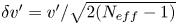 $\delta v'={v'}/{\sqrt {2(N_{eff}-1)}}$, while the uncertainty of the Reynolds shear stress
  $\delta \langle uv \rangle$ is given by
  $\delta \langle uv \rangle = u'v'\sqrt {{1+\rho _{uv}^{2}}/{N_{eff}-1}}$ with
  $\rho _{uv}={\langle uv \rangle }/{u'v'}.$ The uncertainties of the above turbulence statistics at each
  $y$ location have been quantified for all the experimental OCF cases. In summary, the inner-scale normalized uncertainties are very small (
 $\delta U^{+}<0.04$,
  $\delta V^{+}<0.02$,
  $\delta u'^{+}<0.03$,
  $\delta v'^{+}<0.01$ and
  $\delta \langle uv \rangle ^{+}<0.04$).


