2.1. Physical cases

To verify the performance of critical indicators in different flow scenarios and study the influence of parameters, a large number of pitching cases are obtained here. The cases in this study are mainly divided into three groups, namely the cases obtained by the present numerical simulation (Cases 1, 2 and 3), the numerical cases of Narsipur et al. (Reference Narsipur, Hosangadi, Gopalarathnam and Edwards2020) (Cases A, B, C, D and other cases, a total of 115 cases) and a wind tunnel experimental case of Mulleners & Raffel (Reference Mulleners and Raffel2012, Reference Mulleners and Raffel2013) (Case E). The typical motion forms and airfoils of these cases are shown in figure 1, with their motion parameters listed in table 1. Here and below, $\alpha $ is the angle of attack, c is the chord length of the airfoil, x_p/c is the dimensionless pivot location and Re represents the chord-length-based Reynolds number. Parameter ${\omega ^ + }$ is the dimensionless angular velocity $({\omega ^ + } = \omega c/{U_\infty })$, $\omega $ is the dimensional angular velocity of pitch motion and ${U_\infty }$ represents the free-stream velocity. Also, K is the dimensionless pitching rate $(K = \dot{\alpha }c/2{U_\infty })$ and $\dot{\alpha }$ is the dimensional pitching rate. Parameters K and ${\omega ^ + }$ have the same physical meaning, but their values are twice as different. As both expressions are used in different references, both expressions are retained here to be consistent with the references. Parameter k is the reduced frequency, $k = {{\rm \pi} }fc/{U_\infty }$, and f is the frequency of sinusoidal pitching motion.

Figure 1. Variations in the angle of attack with convective time and airfoils of different cases. (a) Case 1, Case 2 and Case 3. (b) Representative cases selected from database N (Narsipur et al. Reference Narsipur, Hosangadi, Gopalarathnam and Edwards2020). (c) Case E (Mulleners & Raffel Reference Mulleners and Raffel2012, Reference Mulleners and Raffel2013).

Table 1. Parameter list of the cases used in this study.

Case 1 has the same motion and parameters as the wind tunnel experimental case of Gupta & Ansell (Reference Gupta and Ansell2018). In this case, a NACA 0012 airfoil experiences a ramp-up motion (figure 1a) from $\alpha = - 6^\circ $ to $\alpha = 30^\circ $ with a constant dimensionless angular velocity of ${\omega ^ + } = 0.05$ and a Reynolds number of $Re = 5 \times {10^5}$. Visbal (Reference Visbal2014), Visbal & Benton (Reference Visbal and Benton2018) and Benton & Visbal (Reference Benton and Visbal2019) also carried out three-dimensional LES studies on cases that have very similar parameters to those of Case 1. Therefore, the basic flow situation of this case is well understood. The motions and parameters of Case 2 and Case 3 are similar to those of Case 1, except that their ${\omega ^ + }$ values are equal to 0.1 and 0.2, respectively.

The database of Narsipur et al. (Reference Narsipur, Hosangadi, Gopalarathnam and Edwards2020) contains a total of 115 numerical cases, all of which adopt pitch-up-return motion (figure 1b). The parameter range includes two Reynolds numbers ($Re = 3 \times {10^4}$ and $Re = 3 \times {10^6}$), two airfoils (NACA 0012 and SD7003m), eight different pitching rates (varying from K = 0.005 to K = 0.6) and five different pivot locations (x_p/c = 0.00, 0.25, 0.50, 0.75 and 1.00, denoted as LE, QC, MC, TQ and TE, respectively). The database of Narsipur et al. (Reference Narsipur, Hosangadi, Gopalarathnam and Edwards2020) provides a very wide parameter envelope, which can be used to widely verify the influence of different parameters on critical indicators. For more details of this database, the reader is referred to the published work of Narsipur et al. (Reference Narsipur, Hosangadi, Gopalarathnam and Edwards2020). In the following, this database is called database N. Cases A, B, C and D are four representative cases selected from database N. Their principles of parameter selection are to be away from those of Cases 1, 2 and 3 and reflect the influence of different parameters as much as possible.

Case E is a classic wind tunnel experimental case, whose flow situation and the variation of the LESP have been reported widely (Mulleners & Raffel Reference Mulleners and Raffel2012, Reference Mulleners and Raffel2013; Deparday & Mulleners Reference Deparday and Mulleners2019; Ansell & Mulleners Reference Ansell and Mulleners2020). In Case E, the OA209 airfoil is selected for sinusoidal pitching motion (figure 1c), with average angle of attack ${\alpha _0} = 20^\circ $, pitching amplitude ${\alpha _m} = 8^\circ $, reduced frequency k = 0.05, Reynolds number Re = 9.2 × 10⁵ and pivot location x_p/c = 0.25. Time-resolved particle image velocimetry measurements and surface pressure measurements based on pressure transducers of Case E have been carried out and can be found in Mulleners & Raffel (Reference Mulleners and Raffel2012, Reference Mulleners and Raffel2013). The distribution of pressure transducers is shown on the right-hand side in figure 1(c). A total of 40 pressure transducers were arranged on the airfoil, including 27 (blue dots) on the suction surface and 13 (open circles) on the pressure surface. The sampling frequency of the pressure signals was 6 kHz, the continuous sampling time was 15 s and the data of 39 cycles were measured. In this study, the 27 transducers on the suction surface are used to construct critical indicators. For the convenience of description, the transducers on the suction surface from the leading-edge point to the trailing-edge point are serially numbered from 1 to 27. These serial numbers are used to refer to the corresponding transducers later.

2.2. Numerical method

In this study, the incompressible unsteady Reynolds-averaged Navier–Stokes (URANS) equation is solved to perform computational fluid dynamics calculations in Cases 1, 2 and 3, and the SST transition model is used. The selected computational domain is a typical O-type grid, with its outer boundary 20c away from the airfoil, and structured grids are used for the whole domain. The distance of the first nodes adjacent to the airfoil surface is small enough so that the condition of y⁺ < 1 is strictly guaranteed. During calculation, the mesh and airfoil rigidly move together. Figure 2(a) shows the results of grid sensitivity verification of Case 1, where the lift coefficients obtained from four different grids are used for comparison. G1, G2, G3 and G4 grids have $5.78 \times {10^5}$, $\; 6.57 \times {10^5}$, $7.37 \times {10^5}$ and $8.16 \times {10^5}$ cells corresponding to 1400, 1600, 1800 and 2000 nodes around the airfoil, respectively. The difference in the lift curves of the four domains mainly exists in the poststall stage. Flow field analysis also shows no significant difference between the calculation results of different grids before DSV detachment. Finally, the G3 grid is selected for subsequent calculations. The time step sensitivity verification is shown in figure 2(b), and all the results in the figure are based on the G3 grid. The influence of the time step on the results is also mainly reflected in the poststall stage. Therefore, the time step size $\Delta t = 0.00005\;\textrm{s}$ is selected for subsequent calculations, corresponding to the non-dimensional time step $\Delta t{U_\infty }/c = 0.00186$. In Cases 1, 2 and 3, at the beginning of the calculation, the airfoil is kept stationary for 0.1 s, and then it starts to pitch up at a constant rate until reaching the maximum angle of attack. In the present simulations, 0.1 s corresponds to 3.72 non-dimensional time units, which is sufficient to develop the flow around the airfoil.

Figure 2. (a) Grid sensitivity verification, (b) timestep sensitivity verification and (c) comparison of the lift coefficient of the present numerical simulation with the experimental results of Gupta & Ansell (Reference Gupta and Ansell2018) and the LES results of Visbal (Reference Visbal2014).

Figure 2(c) shows a comparison of the lift coefficient in Case 1 between the present numerical simulation results, the experimental results of Gupta & Ansell (Reference Gupta and Ansell2018) and the LES results of Visbal (Reference Visbal2014). The lift variation of the present simulation is consistent with the experimental results, and there is only a small difference. As Case 1 contains many complex flow phenomena, such as transition and reattachment, and DSV usually consists of small-scale coherent structures, the small difference between the results obtained using URANS and the experimental results is reasonable, which widely occurs in similar calculations (Wang et al. Reference Wang, Ingham, Ma, Pourkashanian and Tao2010; Amini, Kianmehr & Emdad Reference Amini, Kianmehr and Emdad2019; Narsipur et al. Reference Narsipur, Hosangadi, Gopalarathnam and Edwards2020; Rezaei & Taha Reference Rezaei and Taha2021). Figure 2(c) shows that even the results obtained using the LES also have differences from the experimental results.

The spatiotemporal contours of pressure and skin friction on the suction surface in Case 1 are also shown in figure 3. Gupta & Ansell (Reference Gupta and Ansell2018), Visbal (Reference Visbal2014), Visbal & Benton (Reference Visbal and Benton2018) and Benton & Visbal (Reference Benton and Visbal2019) also display similar figures of the same case. By comparison, it can be found that the evolutions of K–H vortices, LSB, DSV, shear layer vortex and many other flow structures shown in figure 3 are very close to those described by Gupta & Ansell (Reference Gupta and Ansell2018), Visbal (Reference Visbal2014), Visbal & Benton (Reference Visbal and Benton2018) and Benton & Visbal (Reference Benton and Visbal2019). This is another proof of the validity of the present numerical results. On the other hand, this study focuses on the relationship between flow structures such as DSV and airfoil surface pressure, which is the basis of the construction of critical indicators. Because the numerical calculation and the real wind tunnel flow follow the same governing equation, the relationship between the DSV and the surface pressure obtained from the numerical simulation is still valid in the experimental data. Therefore, the small difference between the present numerical results and the experimental results does not affect the nature of this relationship and, therefore, does not affect the conclusions of this study.

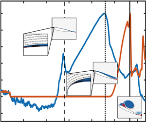
Figure 3. Spatiotemporal contours of (a) pressure coefficient C_p and (b) skin friction coefficient C_f on the suction surface in Case 1. The dashed line, dotted line and solid line from bottom to top correspond to the moments of LSB formation, DSV initiation and DSV detachment, respectively. Region ${\bigcirc{\kern-6pt 1}}$ represents the trace of the K–H vortices, mark ${\bigcirc{\kern-6pt 2}}$ represents the trace of the LSB and mark ${\bigcirc{\kern-6pt 3}}$ represents the DSV-induced pressure wave.

3.1. Basic flow situation

Since the critical moment is closely related to the flow events in the flow field, this section takes Case 1 as an example to briefly introduce its basic flow situation. Figure 3 shows the spatiotemporal contours of the pressure coefficient C_p and skin friction coefficient C_f on the suction surface in Case 1, where ${t^\ast } = t{U_\infty }/c$ represents the dimensionless convection time and ${t^\ast } = 0$ corresponds to the moment when the airfoil starts to move from $\alpha = - 6^\circ $. In this study, x without a subscript represents the chordwise coordinates in the airfoil body coordinate system, y represents the coordinates normal to the chord and the origin of the body coordinate system is fixed at the leading-edge point of the airfoil. The dashed line, dotted line and solid line in figure 3 correspond to the moments of ${t^\ast } = 5.58$, ${t^\ast } = 9.18$ and ${t^\ast } = 11.34$, which represent the formation of LSB, the initiation of DSV and the detachment of DSV, respectively. The quantitative identification methods of these moments are introduced later.

At the beginning of the motion, the flow on the suction surface is attached. With the increase in the angle of attack, separation and reverse flow appear near the trailing edge. As shown in figure 4, at ${t^\ast } = 3.53$, under the effect of K–H instability, the separated shear layer rolls up into K–H vortices, which convect downstream continuously. With flow development, the trailing-edge separation point keeps moving upstream, causing the convective trace of the K–H vortices to occupy most of the suction surface, which can be seen in the skin friction contour in figure 3(b) (region ${\bigcirc{\kern-6pt 1}}$). At ${t^\ast } = 5.58$, the trailing-edge separation point reaches the vicinity of the leading edge for the first time. Simultaneously, an LSB appears at the leading edge and then it remains for some time. The pressure footprint and skin friction trace of the LSB can be seen in figure 3 (mark ${\bigcirc{\kern-6pt 2}}$), and its detailed structure at ${t^\ast } = 7.25$ is also shown in figure 4. After LSB formation, the flow downstream of it reattaches, and a new flow separation point appears downstream of the reattached flow region. During the maintenance of the LSB, this new separation point moves from the trailing edge towards the leading edge continuously. Meanwhile, the LSB shrinks in size and slightly moves upstream. After ${t^\ast } = 9.18$, the LSB bursts, and DSV initiates at the leading edge. Then, with the additional feeding vorticity from the shear layer, the circulation and size of the DSV increase significantly, and the position of its centre moves downstream. The convection of the DSV induces a strong pressure wave on the suction surface, as shown in figure 3(a) (mark ${\bigcirc{\kern-6pt 3}}$). This pressure wave is the most distinctive pressure footprint of the DSV. In addition, there is a large-scale shear layer vortex downstream of the DSV, which grows and convects with the growth of the DSV. Figure 4 shows detailed structures of the DSV and the shear layer vortex at ${t^\ast } = 9.48$ and ${t^\ast } = 10.23$. During the development of the DSV, upstream of the DSV and beneath the leading-edge shear layer, the secondary vorticity accumulates continuously and eventually erupts and pinches off the DSV from its shear layer, resulting in the detachment of the DSV $({t^\ast } = 11.34)$.

Figure 4. Vorticity contours of the flow field at some representative moments, with streamlines being plotted. The right-hand panels are enlargements of the black boxes in the left-hand panels.

3.2. The criterion of LSB formation time

The purpose of this study is to establish some critical indicators using the pressure information on the airfoil surface and hope that these indicators can be calculated in real time so that they can be used as the feedback or reference frame of flow control. Therefore, based on the identification of the flow field, some non-real-time methods need to be developed, which are used to accurately determine the occurrence moment of critical flow events. These moments are the verification criteria for the accuracy of critical indicators. This section introduces the identification method of LSB initiation. Sections 3.3 and 3.4 introduce the identification method of DSV initiation and DSV detachment, respectively.

Figure 5 shows the vorticity contours and streamlines near the leading edge at ${t^\mathrm{\ast }} = 5.39$, ${t^\mathrm{\ast }} = 5.58$ and ${t^\mathrm{\ast }} = 5.76$, as well as the skin friction distribution near the leading edge in Case 1. At ${t^\mathrm{\ast }} = 5.39$, there is no LSB in the flow field. In the range of approximately 0.04 < x/c < 0.12, there is a negative region of C_f, which indicates that the trailing-edge separation point approaches near the leading edge for the first time. In areas further downstream, C_f alternates between positive and negative values due to the existence and convection of K–H vortices. At ${t^\mathrm{\ast }} = 5.58$, an LSB can be recognized in the flow field first, which corresponds to the appearance of an inflection point in the negative-C_f region for the first time (figure 5b). This inflection point is actually due to the accumulation of positive vorticity (red region) upstream of the LSB. In the description of Narsipur et al. (Reference Narsipur, Hosangadi, Gopalarathnam and Edwards2020), it is found that the event whereby the inflection point appears in the negative-C_f region for the first time corresponds to the initiation of DSV. This is because an LSB is not observed in the cases of Narsipur et al. (Reference Narsipur, Hosangadi, Gopalarathnam and Edwards2020), and many characteristics of DSV at the initial time are similar to those of LSBs observed in this study. However, the difference between them is that the DSV continues to grow and convect downstream; in contrast, the LSB does not grow but shrinks in size and slightly moves upstream, as shown in figure 5(c). Therefore, ${t^\mathrm{\ast }} = 5.58$ is regarded as the formation time of the LSB in Case 1. In the following, the formation time of the LSB in all cases is denoted as $t_1^\ast $.

Figure 5. Vorticity contours with streamlines (left and middle columns) and skin friction coefficient (right column) in the range x = 0–0.25c at several moments before and after LSB initiation in Case 1: (a) ${t^\ast } = 5.39$, (b) ${t^\ast } = 5.58$ and (c) ${t^\ast } = 5.76$. The centre panels are enlargements of the black boxes in the left-hand panels.

3.3. The criterion of DSV initiation time

In previous literature, it is a common method to use some critical events of the skin friction on the suction surface as the basis to identify the initiation time of DSV. However, in different cases, the specific method is different. Ramesh et al. (Reference Ramesh, Granlund, Ol, Gopalarathnam and Edwards2018) and Hirato et al. (Reference Hirato, Shen, Gopalarathnam and Edwards2021) used the event that ‘the value of the inflection point in the negative-C_f region changes to positive for the first time’ as the criterion of DSV initiation. In Case 1, when this skin friction event happens, DSV has developed for a period and already has a large size (figure 6d). Therefore, the method of Ramesh et al. (Reference Ramesh, Granlund, Ol, Gopalarathnam and Edwards2018) and Hirato et al. (Reference Hirato, Shen, Gopalarathnam and Edwards2021) is too late to be used as the best criterion of DSV initiation in Case 1. Narsipur et al. (Reference Narsipur, Hosangadi, Gopalarathnam and Edwards2020) used the event of ‘the inflection point appears in the negative-C_f region for the first time’ as the criterion of DSV initiation. However, as has been demonstrated in § 3.1, this method corresponds to the formation of an LSB, which is too early to be a criterion of DSV initiation in Case 1. Therefore, for the flow situation of Cases 1, 2 and 3, a more accurate criterion for DSV initiation is needed.

Figure 6. Vorticity contours with streamlines (left and middle columns) and skin friction coefficient (right column) near the leading-edge region at several moments before and after DSV initiation in Case 1: (a) ${t^\ast } = 8.92$, (b) ${t^\ast } = 9.18$, (c) ${t^\ast } = 9.39$ and (d) ${t^\ast } = 9.85$. The centre panels are enlargements of the black boxes in the left-hand panels.

During the existence of the LSB, it causes a ‘spike’ in the negative-C_f region, as shown in figure 6(a). Since the flow separates upstream of the LSB and reattaches downstream, the downstream region of the LSB corresponds to a positive region of C_f. With flow development, the reverse flow region expands upstream and interferes with the LSB at ${t^\mathrm{\ast }} = 9.18$, resulting in the bursting of the LSB. This phenomenon corresponds to the change in C_f from positive to negative in the region immediately downstream of the LSB (figure 6b). Following LSB bursting, the complete structure of DSV can be identified directly in the flow field at ${t^\mathrm{\ast }} = 9.39$. However, no obvious critical skin friction event is observed at $t^{\ast} = 9.39$. Therefore, it is difficult to identify this moment quantitatively through C_f. In addition, considering that the works of Benton & Visbal (Reference Benton and Visbal2019) and Sharma & Visbal (Reference Sharma and Visbal2019) have shown the close physical relationship between ‘LSB collapse’ and ‘DSV initiation’, as well as the high similarity of the occurrence time of these two events, the bursting of the LSB is also regarded as the landmark of DSV initiation in this study. In figure 6(b), the LSB bursting corresponds to the event that the positive C_f region immediately downstream of the LSB becomes negative for the first time. Therefore, this skin friction event can be regarded as a symbol of DSV initiation. In the following, the initiation moment of DSV is denoted as $t_2^\ast $.

3.4. The criterion of DSV detachment time

In addition to the formation of the LSB and DSV, another important critical event is the detachment of the DSV. In Case 1, the shedding mechanism of the DSV is closer to the boundary layer eruption mechanism mentioned by Widmann & Tropea (Reference Widmann and Tropea2015). DSV shedding can be described as a process in which the leading-edge shear layer stops feeding circulation to the DSV (Ringuette, Milano & Gharib Reference Ringuette, Milano and Gharib2007; Huang & Green Reference Huang and Green2015). Therefore, the time when the DSV is pinched off from the leading-edge shear layer is defined as the DSV detachment time here.

Figure 7 shows the vorticity contours and skin friction distribution on the suction surface at different moments before and after DSV detachment. At ${t^\mathrm{\ast }} = 10.97$ (figure 7a), the DSV is still in growth and has not been pinched off from the leading-edge shear layer. At this time, the trace of DSV is visible in the distribution of C_f. At ${t^\mathrm{\ast }} = 11.15$ (figure 7b), it can be found from the vorticity contour that the leading-edge shear layer is still feeding vorticity to the DSV. At ${t^\mathrm{\ast }} = 11.34$ (figure 7c), the DSV is in the process of being pinched off, most of the vorticity from the leading-edge shear layer is feeding into the newly formed LEV and the secondary vorticity is erupting rapidly. At ${t^\mathrm{\ast }} = 11.53$ (figure 7d), the DSV has been pinched off from the leading-edge shear layer and begins to convect downstream. At ${t^\mathrm{\ast }} = 11.71$ (figure 7e), the DSV moves away from the airfoil surface after its detachment, its strength gradually dissipates and the trace of DSV in the C_f distribution is no longer apparent. Based on these observations, ${t^\mathrm{\ast }} = 11.34$ can be regarded as the reference time of DSV detachment in Case 1. In the following text, the reference time of DSV detachment is denoted as $t_3^\ast $. Furthermore, a more certain fact is that the critical event of DSV detachment should be in the range $11.15 < {t^\mathrm{\ast }} < 11.53$. Therefore, the time range $11.15 < {t^\mathrm{\ast }} < 11.53$ can be taken as an error interval of DSV detachment.

Figure 7. Vorticity contours (left column) and skin friction coefficient (right column) on the suction surface at several moments around DSV detachment in Case 1: (a) ${t^\mathrm{\ast }} = 10.97$, (b) ${t^\mathrm{\ast }} = 11.15$, (c) ${t^\mathrm{\ast }} = 11.34$, (d) ${t^\mathrm{\ast }} = 11.53$ and (e) ${t^\mathrm{\ast }} = 11.71$.

Figure 8(a) shows the variation in the normal distance y_v between the DSV centre and the airfoil chord line with ${t^\mathrm{\ast }}$, and figure 8(b) shows the variation in the absolute value of DSV circulation. The black vertical line in the figure is the reference time of DSV detachment $t_3^\ast $. In these calculations, the vortex is distinguished from the velocity field by the ${\lambda _{ci}}$ criterion (Zhou et al. Reference Zhou, Adrian, Balachandar and Kendall1999), where the connected domain with ${\lambda _{ci}}\; \ge 1\;{\textrm{s}^{ - 1}}$ is regarded as the interior of the vortex. The determination of this threshold is based on the work of Li et al. (Reference Li, Feng, Kissing, Tropea and Wang2020). The position of the vortex centre is determined by the ${\varGamma _1}$ criterion proposed by Graftieaux, Michard & Nathalie (Reference Graftieaux, Michard and Nathalie2001). Within the vortex boundary, the local maximum of the scalar function ${\varGamma _1}$ is regarded as the vortex centre, and the circulation of DSV is obtained by the integral of the vorticity. As can be seen from figure 8(a), y_v increases linearly with time before and after $t_3^\ast = 11.34$, indicating that the DSV starts to move away from the wall rapidly after $t_3^\ast $. As can also be seen from figure 8(b), before $t_3^\ast $, the circulation of the DSV has been increasing continuously, but it keeps constant for a while after $t_3^\ast $ and begins to decrease after ${t^\mathrm{\ast }} = 11.71$ because of the dissipation of vorticity. All these results support the above identification of $t_3^\ast = 11.34$ as the reference time of DSV detachment.

Figure 8. Variation in (a) the normal distance from the DSV centre to the airfoil chord line and (b) DSV circulation with ${t^\mathrm{\ast }}$ in Case 1. The solid black line represents the reference time of DSV detachment.

In §§ 3.2–3.4, the identification methods of LSB formation, DSV initiation and DSV detachment are discussed. In the following, these three critical moments are denoted as $t_1^\ast $, $t_2^\ast $ and $t_3^\ast $, respectively, which are also used in other cases.

4.1. Evolution of surface pressure

In the process of dynamic stall, the variation in the pressure distribution on the suction surface can fully reflect the status of the near-wall flow field. Therefore, abundant information about the flow criticality can be obtained by measuring and analysing the pressure distribution variation on the suction surface. Figure 9 shows the spatial and statistical distribution of the pressure coefficient on the suction surface at several representative moments in Case 1. The statistical distribution is the probability density distribution of C_p data from all measuring points at a certain time, whose detailed definition is as follows: at time ${t^\ast }$, the C_p from all measuring points constitutes a group of sample data (${C_{p,1}}({t^\ast })$, ${C_{p,2}}({t^\ast }), \ldots {C_{p,N}}({t^\ast })$, where N is the number of measuring points). Calculating the distribution probability of this group of sample data in different value intervals is the named statistical distribution of C_p at this time. At ${t^\mathrm{\ast }} = 3.53$, as most of the flow on the suction surface is attached, the spatial distribution of pressure is relatively flat, except for the small fluctuations near the trailing edge caused by K–H vortices. At this time, the statistical distribution of pressure is concentrated in a small range and approximately uniform. At $t_1^\ast = 5.58$, a negative peak pressure appears at the leading edge. The LSB has just formed, and a pressure plateau caused by the LSB is present. Simultaneously, the dispersion, kurtosis and skewness of the statistical pressure distribution begin to increase. With the increase in the angle of attack, the leading-edge negative peak pressure increases continuously, and the statistical pressure distribution keeps its previous variation trend until DSV initiation. At $t_2^\ast = 9.18$ when the DSV initiates, the leading-edge negative peak pressure is highly concentrated, and the statistical distribution of pressure has the maximum dispersion, kurtosis and skewness. After DSV initiation, the negative peak pressure collapses rapidly. With the growth and convection of DSV, the location of the negative peak pressure also moves downstream. At $t_3^\ast = 11.34$, the reference time of DSV detachment, the negative peak pressure is no longer apparent, and the spatial pressure distribution becomes flat again. Accordingly, the dispersion, kurtosis and skewness of the statistical distribution of pressure also decrease.

Figure 9. Spatial distribution (left column) and statistical distribution (right column) of the pressure coefficient on the suction surface at (a) ${t^\mathrm{\ast }} = 3.53$, (b) ${t^\mathrm{\ast }} = 5.58$, (c) ${t^\mathrm{\ast }} = 9.18$ and (d) ${t^\mathrm{\ast }} = 11.34$ in Case 1.

Although the above analysis of surface pressure evolution characteristics is based on Case 1, the evolution of DSV in different cases is generally similar. Therefore, in other cases, the basic variation in pressure is still qualitatively consistent to a great extent. To better understand the relationship between flow criticality and surface pressure, it is necessary to use mathematical methods to establish the quantitative relationship between them. Proper orthogonal decomposition (POD) is a technique for low-order analysis that extracts modes by optimizing the mean square of measured field variables. Modern POD applications are dedicated to exploring space–time separation and can be used as a method to extract coherent structures from turbulent flows (Taira et al. Reference Taira, Brunton, Dawson, Rowley, Colonius and Mckeon2017). Note that the definition of the pressure coefficient ${C_p}$ is the fluctuation of the pressure at a certain point relative to that of the free stream. Thus, the pressure coefficient data on the suction surface are directly used for POD analysis to extract the characteristic modes corresponding to various critical events.

Figure 10 shows the first 16 spatial POD modes of C_p on the suction surface and their corresponding normalized time coefficients in Case 1. The dotted line, the dashed line and the solid line in the figure represent the $t_1^\ast $, $t_2^\ast $ and $t_3^\ast $ moments, respectively, and the same lines are also plotted in the following figures. Figure 10(a) shows that the first spatial mode represents a gentle pressure distribution on the suction surface, and the variation of its time coefficient is very close to that of the lift coefficient in this case (the lift coefficient can be seen in figure 13). The pressure distribution of the second spatial mode is mainly reflected in the negative peak pressure with a high concentration at the leading edge. Moreover, the maximum value of the time coefficient of this mode corresponds to time $t_2^\ast $, coinciding with the phenomenon that the leading-edge negative peak pressure reaches the maximum at time $t_2^\ast $. Both the third and fourth spatial modes show a negative peak pressure, which is flatter than the leading-edge peak in the second spatial mode. However, the location of the peaks in the third and fourth spatial modes is not at the leading edge. Combined with the cognition of flow, it can be inferred that these two modes are related to DSV. In addition, the time coefficients of the third and fourth modes begin to rapidly increase shortly after $t_2^\ast $, reach the maximum value in the middle of the $t_2^\ast \text{--} t_3^\ast $ interval and fall rapidly shortly before $t_3^\ast $. From figure 3(a), it can be seen that the surface pressure induced by the DSV also gradually increases after $t_2^\ast $. However, it does not continuously increase during the existence of DSV but reaches the strongest at one intermediate time of the $t_2^\ast \text{--} t_3^\ast $ interval and rapidly decreases near $t_3^\ast $. This phenomenon further confirms the direct correlation between the third and fourth modes and the DSV.

Figure 10. The first 16 POD spatial modes (left column) and their corresponding normalized time coefficients (right column) of the pressure coefficient on the suction surface in Case 1.

In figure 10(b), the fifth to eighth modes have smaller eigenvalues than the first four modes. Therefore, these modes represent the pressure fluctuations caused by the lower-energy flow structures, which are not concentrated on the leading edge but oscillate over the whole airfoil. In addition, the time coefficients of the fifth to eighth modes are relatively stable and close to zero before $t_2^\ast $, and all of them have a local extremum around $t_2^\ast $ and then begin to oscillate violently. The existence of the local extrema of the fifth to eighth modes around $t_2^\ast $ implies an important fact that the pressure outside the leading edge may also contain some information about DSV initiation. That is, although the flow criticality at the leading edge has always been considered a causal factor for the initiation of DSV or dynamic stall onset in the past, the flow criticality outside the leading edge, as has been shown here, may also have a contribution to the initiation of DSV. The causality between the flow criticality outside the leading edge and DSV initiation is a discovery in this study, which is also a theoretical basis for using the pressure on the whole suction surface to construct the critical indicators.

Figures 10(c) and 10(d) show the 9th–16th spatial modes and their time coefficients. These modes have lower energy levels, so they can be considered to represent the influence of various small-scale flow structures in the flow field. Among them, the time coefficients of the 9th, 10th and 11th modes still have a local extremum around $t_2^\ast $, but the time coefficients of the higher modes have no apparent characteristics around $t_2^\ast $. In addition, an important phenomenon is that all the time coefficients of the 9th–16th modes have a local extremum or mutation around $t_1^\ast $. This result shows that the flow criticality at $t_1^\ast $ is also reflected in the surface pressure and is mainly related to some small-scale flow structures. Moreover, although $t_1^\ast $ corresponds to LSB formation, it can be seen that the pressure fluctuations reflected by these high-order modes are not concentrated in the leading-edge region where the LSB is located but distributed over the whole suction surface. This kind of flow criticality reflected in the high-order modes around $t_1^\ast $ is also the theoretical basis for establishing the critical indicators that can predict the formation of the LSB.

To further confirm the relationship between the mathematical structures of POD modes and the physical structures in the flow field, the spatiotemporal contours of the reconstructed C_p based on different modes are shown in figure 11. By comparing the panels in figure 11 with figure 3(a), it can be found that different modes are associated with different flow structures. Figure 11(a) shows the pressure contours reconstructed by the first and second modes. As mentioned above, the first mode represents the overall variation in pressure, while the second mode represents the concentration of leading-edge negative pressure. Therefore, figure 11(a) shows the overall variation in pressure during dynamic stall and the uplift and collapse of the leading-edge negative pressure. Figure 11(b) shows the pressure reconstruction of the third and fourth modes, and therefore this contour mainly reflects the pressure wave induced by the DSV and the high-pressure region caused by the flow entrainment of the DSV. Figure 11(c) shows the reconstructed pressure contours based on the fifth and all of the higher-order modes. Although the concentration of leading-edge negative pressure and the traces of DSV-induced pressure waves are not apparent, the traces of LSB and K–H vortices are visible, confirming the above judgment that higher-order modes are associated with small-scale structures. In general, the results of figure 11 have fully proven that the different POD modes can indeed correspond to various specific flow structures. This relationship implies that the flow evolution in the dynamic stall can be described by individual simplified physical schemas.

Figure 11. Spatiotemporal contours of the reconstructed C_p on the suction surface in Case 1. (a) Reconstruction based on the first and second modes, (b) reconstruction based on the third and fourth modes and (c) reconstruction based on the fifth and all of the higher-order modes.

Based on the understanding of the pressure characteristics during dynamic stall, and inspired by the results of figure 11, the evolution of the pressure on the suction surface during dynamic stall is summarized into three intuitive and basic physical schemas here: (i) concentration of leading-edge negative pressure, (ii) downstream movement of negative peak pressure and (iii) small-amplitude fluctuations of pressure. During the whole dynamic stall process, the pressure evolution on the suction surface can be regarded as alternating or combining these three physical schemas. Figure 12 shows their schematic diagrams. The spatial pressure distributions at five different moments are given in each panel, and each line represents the spatial pressure distribution on the suction surface at a certain time. In the first schema, the concentration of leading-edge negative pressure mainly exists before DSV initiation. In figure 12(a), for simplicity, the pressure distribution is directly simplified to a linear form to characterize the macroscopic trend. The validity and rationality of this simplification are further explained in § 6.1. The second schema shown in figure 12(b) mainly depicts the influence of DSV or subsequent LEVs, so it is predominant after DSV initiation. Figure 12(c) shows that the third schema mainly reflects the pressure fluctuations caused by various small-scale flow structures. This schema exists in the whole process of dynamic stall, but its intensity and form in different stages are different, and the amplitudes of the sine waves in figure 12(c) should be far less than the pressure fluctuation amplitudes expressed in the first and second schemas. It can be speculated that some critical indicators related to dynamic stall could be constructed by measuring these three basic physical schemas.

Figure 12. Three basic physical schemas of the pressure evolution on the suction surface in the dynamic stall process: (a) concentration of leading-edge negative pressure, (b) downstream movement of negative peak pressure and (c) small-amplitude fluctuations of pressure. The grey arrows in (a, b) represent the chronological order.

4.2. Spatial distribution coefficient of pressure

To characterize the above three basic physical schemas uniformly and quantitatively, a new critical indicator, the SDCP, is proposed to depict the variation in spatial pressure distribution. Suppose that N_s pressure transducers are distributed on the suction surface of the airfoil from the leading edge to the trailing edge, the serial number of which is n = 1, 2, 3, … N_s. The pressure coefficient of the nth transducer at ${t^\ast }$ is denoted as ${C_{p,n}}({t^\ast })$, the chordwise dimensionless coordinate of this transducer is denoted as $x_n^\ast $, where $x_n^\ast = {x_n}/c$, and then the SDCP is defined as

(4.1) \begin{align}\textrm{SDCP}({t^\ast }) &= \sum\limits_{n = 1}^{{N_s} - 1} {[{C_{p,n + 1}}({t^\ast }) - {C_{p,n}}({t^\ast })]}\times (1 - x_n^\ast )^{{\textrm{sgn(}{C_{p,n + 1}}({t^\ast }) - {C_{p,n}}({t^\ast })\textrm{)}}}{x}_{n}^{\ast} {}^{[1 -\textrm{sgn}(C_{p,n + 1}(t^\ast)-C_{p,n}(t^\ast))]},\end{align}

where ‘sgn’ is the standard symbolic function, which is defined as

(4.2) \begin{equation}\textrm{sgn}(x) = \left\{ {\begin{array}{@{}ll} {1,}&{\textrm{if}\;x \ge 0}\\ {0,}&{\textrm{if}\;x < 0.} \end{array}} \right.\end{equation}

Equation (4.1) gives the definition of SDCP when discretely distributed transducers are used. However, when spatially continuous pressure data are used, the number of transducers N_s tends to infinity, and therefore the expression of SDCP becomes

(4.3) \begin{align}\mathop {\lim }\limits_{{N_s} \to \infty } \textrm{SDCP}({t^\mathrm{\ast }}) = \int_0^1 {\frac{{\partial {C_p}({x^\mathrm{\ast }},{t^\mathrm{\ast }})}}{{\partial {x^\mathrm{\ast }}}}} {(1 - {x^\mathrm{\ast }})^{\textrm{sgn(}\partial {C_p}\textrm{(}{x^\mathrm{\ast }},\,{t^\mathrm{\ast }}\textrm{)/}\partial {x^\mathrm{\ast }})}}{x^{\mathrm{\ast }[1 - \textrm{sgn}(\partial {C_p}({x^\mathrm{\ast }},\,{t^\mathrm{\ast }})/\partial {x^\mathrm{\ast }})]}}\,\textrm{d}\kern0.7pt{x^\mathrm{\ast }},\end{align}

where $\partial {C_p}({x^\mathrm{\ast }},{t^\mathrm{\ast }})/\partial {x^\mathrm{\ast }}$ is the spatial partial derivative of ${C_p}({x^\mathrm{\ast }},{t^\mathrm{\ast }})$. Although the expression of SDCP in (4.3) includes the derivative, it is just the extreme situation when the number of transducers tends to infinity. It is shown later that the SDCP is not particularly sensitive to noise when it is calculated using instantaneous wind tunnel experimental data measured by a limited number of transducers.

As mentioned above, the pressure evolution on the suction surface in the dynamic stall process can be summarized into three basic physical schemas. According to our further verification, the SDCP changes regularly with the main parameters in these three schemas. For example, in the first physical schema, the SDCP increases with an increase in leading-edge negative peak pressure; in the second schema, the SDCP decreases with the downstream movement of the negative peak pressure; in the third schema, the SDCP increases with an increase in the frequency and amplitude of the sine waves. Therefore, the SDCP can characterize these three basic physical schemas, demonstrating that the SDCP can characterize the actual pressure evolution in the dynamic stall process and predict the critical flow event.

Figure 13 shows the variation in the lift coefficient C_L and SDCP with ${t^\ast }$ in Case 1. For the convenience of display, the lift coefficient and indicator SDCP are normalized by dividing their maximum values. Here and below, all the data in the figures whose ordinate is ‘normalized value’ adopt such a normalized method. As shown in figure 13, when the airfoil starts to pitch up from α = −6° (t* = 0), the SDCP first decreases with fluctuations. As the time approaches $t_1^\ast $, the SDCP rises rapidly, and a sharp local peak appears just before $t_1^\ast $. Then, the SDCP continues to rise after a short descent and reaches the maximum around $t_2^\ast $. After $t_2^\ast $, the SDCP continues to decrease shortly before the DSV detachment, denoted by $t_3^\ast $, and then a local peak value appears again. The fact that the SDCP has a local peak or maximum at approximately $t_1^\ast $ and $t_2^\ast $ is of great significance, which means that the SDCP marks the occurrence of two critical flow events, namely LSB formation and DSV initiation. Moreover, the SDCP reflects the internal relationship between these two flow events from the view of pressure.

Figure 13. Variation in C_L and SDCP with time in Case 1.

Although the SDCP has a local peak around both $t_1^\ast $ and $t_2^\ast $, the physical mechanism behind them is different. At moment $t_1^\ast $, the first basic physical schema shown in figure 12(a) is still developing continuously and has not reached the critical state. Simultaneously, the second physical schema has not yet appeared. Therefore, the local peak of the SDCP around $t_1^\ast $ mainly reflects the criticality of the third schema, which corresponds to the extremums or mutations of the time coefficients of high-order modes around $t_1^\mathrm{\ast }$ in the pressure POD analysis. Before moment $t_2^\ast $, no massive flow separation is observed at the leading edge, and the leading-edge negative peak pressure is constantly uplifted; thus, the pressure evolution is dominated by the first physical schema. However, after $t_2^\ast $, the leading-edge negative peak pressure has collapsed, and the DSV has formed. With the aftward movement of the negative peak pressure location, the pressure evolution begins to be dominated by the second physical schema. The local peak of the SDCP around $t_2^\ast $ reflects the transition from the first physical schema to the second physical schema.

4.3. High-order central moment of pressure

Figure 9 shows that the statistical distribution of surface pressure also changes with the flow evolution during the dynamic stall process. Therefore, using statistics to measure the variation in the pressure coefficient can also predict the occurrence of critical flow events. Here, the HCMP is used as the statistic. In the calculation of HCMP, the pressure coefficient data from different spatial measurement points are used, and the mathematical definition of the HCMP is

(4.4)\begin{equation}\textrm{HCMP(}{t^\ast }\textrm{)} = \frac{1}{{{N_s}}}\sum\limits_{n = 1}^{{N_s}} {{{\{ [ - {C_{p,n}}({t^\ast })] - [ - \overline {{C_p}({t^\ast })} ]\} }^m}} ,\end{equation}

where m is the order of the moment, prescribing that m ∈ N⁺, and m > 1. In (4.4), $\overline {{C_p}({t^\ast })} $ represents the average value of the pressure coefficient from all pressure transducers at a certain time:

(4.5)\begin{equation}\overline {{C_p}({t^\mathrm{\ast }})} = \frac{1}{{{N_s}}}\sum\limits_{n = 1}^{{N_s}} {{C_{p,n}}({t^\mathrm{\ast }})} .\end{equation}

Figure 14 shows the variation in the HCMP of different orders with ${t^\mathrm{\ast }}$ in Case 1. When m = 2, the maximum value of the HCMP is between $t_2^\ast $ and $t_3^\ast $, which cannot correctly reflect the criticality of flow. When $m \ge 3$, the maximum value of the HCMP is always around moment $t_2^\ast $. Moreover, the higher the order is, the narrower the peak of the HCMP is, and the smoother the curve is in the poststall stage. Although only HCMPs with orders less than 16 are shown in the figure, HCMPs with larger orders have similar properties. The results of figure 14 indicate that the HCMP can be used as a critical indicator to predict DSV initiation. In the following, the 16th-order HCMP is used by default.

Figure 14. Variation in C_L and HCMP of different orders with time in Case 1. The dashed line, dotted line and solid line correspond to the moments of LSB formation, DSV initiation and DSV detachment, respectively.

The definition of HCMP only uses the central moment as the statistic, which is one of the most basic statistics. In mathematics, many statistics can be constructed based on the central moment. Therefore, in addition to the HCMP, there should be more statistical indicators that can be used to indicate the flow criticality at $t_2^\ast $.

4.4. Location of peak pressure

As mentioned above, after its initiation, the DSV experiences a process of continuous growth and convection downstream. It is possible to monitor the flow state of the DSV in the process of convection using its pressure footprint left on the wall. In the convection process, the most obvious trace left by the DSV on the surface is a strong pressure wave. In figure 3(a), the propagation of this pressure wave in Case 1 can also be seen clearly. This pressure wave is very common in different cases with different parameters, even with different motion kinematics. Therefore, it is feasible to use the pressure wave to monitor the state of the DSV in the convection process and the associated critical events in a very wide range of flow scenarios.

To capture the position of the pressure wave in real time by pressure transducers, a simple definition is introduced here. The weighted average chordwise coordinates of the 10 % measurement point with the strongest negative pressure at each moment are taken as the LPP. The determination of the value of 10 % is based on the estimation of the spatial scale of the core region of DSV-induced negative pressure wave. According to the present study, a slight change in this value will not affect the effectiveness of the LPP indicator. Assuming that at time ${t^\ast }$ the serial number of the 10 % transducers with the strongest negative pressure on the suction surface is n = 1, 2, 3, … N_{max 10%}, where N_{max 10%} is equal to the rounding of N_s × 10 %, then the mathematical expression of LPP is

(4.6)\begin{equation}\textrm{LPP}({t^\ast }) = \frac{{\sum\limits_{n = 1}^{{N_{max10\,\%}}} {{C_{p,n}}(x_n^\ast ,{t^\mathrm{\ast }})x_n^\ast } }}{{\sum\limits_{n = 1}^{{N_{max10\,\%}}} {{C_{p,n}}(x_n^\ast ,{t^\mathrm{\ast }})} }}.\end{equation}

Figure 15 shows the variation in LPP during the existence of the DSV in Case 1. The blue line in the figure represents the chordwise coordinates of the position of the DSV centre, x_v, identified from the flow field by the ${\varGamma _1}$ criterion. At $t_2^\ast $ moment, the position of the DSV centre is close to the leading edge, so x_v is close to zero. At this time, LPP is also at a small value due to the existence of the leading-edge negative peak pressure. Before $t_3^\ast $, the values of LPP and x_v are always close to each other and increase with time together. This result shows that the LPP can effectively identify the chordwise position of the DSV centre before DSV detachment. After $t_3^\ast $, the values of LPP and x_v begin to deviate. This is because the DSV continues to move downstream after detachment, but the negative surface pressure induced by the DSV weakens rapidly with DSV away from the airfoil. On the other hand, the newly formed LEVs make the strongest negative pressure appear near the leading edge again, which leads to a decrease in LPP.

Figure 15. Variation in the chordwise position of the DSV centre and LPP with time in Case 1.

4.5. Modulated location of peak pressure

Figure 15 shows that before DSV detachment, the value of LPP coincides with the position of the DSV centre, but they deviate rapidly after DSV detachment. Therefore, using this characteristic of LPP, the time of DSV detachment can be monitored. Figure 16(a) shows the variation in LPP with time in the whole process of dynamic stall. The LPP is close to zero for a long time before $t_2^\ast $, but it begins to rise after $t_2^\ast $ and reaches a local peak at approximately $t_3^\ast $. After DSV detachment, the value of LPP decreases rapidly. However, due to the formation of trailing-edge vortices in the later stage, the value of LPP increases again and reaches a maximum until the end of the motion.

Figure 16. Variation in C_L and (a) LPP and (b) MLPP with time in Case 1.

Although the variation in LPP can effectively reflect the criticality of DSV detachment, to identify the $t_3^\ast $ moment more clearly, the LPP can be further modulated to make its peak value at $t_3^\ast $ more obvious. Figure 17 shows the spatiotemporal contour of the root-mean-square value of the pressure coefficient (C_p,RMS) on the suction surface. The definition of C_p,RMS used in this study is

(4.7)\begin{equation}{C_{p,RMS}}({x^\mathrm{\ast }},{t^\mathrm{\ast }}) = \sqrt {\frac{1}{{\Delta {t^\mathrm{\ast }}}}\int_{{t^\mathrm{\ast }} - \Delta {t^\mathrm{\ast }}}^{{t^\mathrm{\ast }}} {{{[{C_p}({x^\mathrm{\ast }},{t^\mathrm{\ast }}) - \overline {{C_p}({x^\mathrm{\ast }},{t^\mathrm{\ast }})} ]}^2}\,\textrm{d}{t^\ast }} } ,\end{equation}

where $\overline {{C_p}({x^\mathrm{\ast }},{t^\mathrm{\ast }})} $ is the sliding average value of the pressure coefficient at ${x^\mathrm{\ast }}$ in the period of $\Delta {t^\mathrm{\ast }}$ and $\Delta {t^\mathrm{\ast }}$ is the dimensionless time interval defining the filtering process, with $\Delta {t^\mathrm{\ast }} = 1$ here. Equation (4.7) follows the definition method of Benard et al. (Reference Benard, Cattafesta, Moreau, Griffin and Bonnet2011). In this definition, the calculation of C_p,RMS only needs the historical value and current value of the surface pressure at a particular time so that it can be calculated in real time.

Figure 17. Spatiotemporal contour of C_p,RMS in Case 1. The abnormality of ${C_{p,RMS}}$ during $0 < {t^\mathrm{\ast }} < 1$ is due to the starting acceleration at ${t^\mathrm{\ast }} = 0$, which causes very large added-mass forces and surface pressure at this moment.

It can be seen from figure 17 that during the whole motion, C_p,RMS on the front section of the airfoil is at its largest during a period before and after DSV detachment. This high-peak region provides a window containing DSV detachment. Therefore, the LPP can be modulated by C_p,RMS to obtain the MLPP, which is defined as

(4.8)\begin{equation}\textrm{MLPP}({t^\mathrm{\ast }}) = \textrm{LPP}({t^\mathrm{\ast }})\times {\sum\limits_{n = 1}^{{N_s}} {{{[{C_{p,RMS}}(x_n^\ast ,{t^\mathrm{\ast }})]}^m}} },\end{equation}

where the mth power of C_p,RMS is used to modulate the LPP and the power exponent m is an empirical parameter to control the degree of modulation. In this study, m is taken as 3 uniformly in all cases. Figure 16(b) shows the variation in MLPP in Case 1. After modulation, the peak value of MLPP around $t_3^\ast $ is more obvious than that of LPP, which is more conducive to accurate identification. Therefore, it is feasible to predict DSV detachment using MLPP.

In this section, critical indicators SDCP, HCMP, LPP and MLPP are proposed. These four critical indicators can accurately predict the critical moments of LSB formation, DSV initiation, position of the DSV centre and DSV detachment. In addition to the above results, Appendix A further presents the influence of motion unsteadiness in Case 2 and Case 3, and the applicability of these critical indicators has been further confirmed. Appendix B verifies the critical indicators in Cases A–D. These results have proven that the present critical indicators are not only applicable to a few individual cases but also have a wide range of universality.

6.1. Test on Case 1

The influence of the number of transducers on the critical indicators is further discussed in this section. Figure 20 shows the variations in SDCP, HCMP, LPP and MLPP in Case 1 when the number of pressure transducers N_s is equal to 40, 20, 6 and 2. Here, the transducers are always uniformly distributed from the leading edge to the trailing edge. When N_s = 40, the SDCP, HCMP, LPP and MLPP are almost similar to the situation of continuous pressure being used. However, although the SDCP can still accurately predict $t_2^\ast $, its local peak at approximately $t_1^\ast $ is no longer obvious. According to the LES results of Visbal (Reference Visbal2014), Visbal & Garmann (Reference Visbal and Garmann2018), Benton & Visbal (Reference Benton and Visbal2019) and Sharma & Visbal (Reference Sharma and Visbal2019), the minimum scale of LSB can contract to the order of O(0.01c). In addition, from the results of the POD analysis above, it is known that the flow criticality at $t_1^\ast $ is mainly related to some small-scale flow structures. Therefore, it is reasonable that discrete pressure transducers cannot accurately capture the information of LSB and other small-scale structures. When N_s = 20, the SDCP and HCMP can still accurately predict DSV initiation. The LPP and MLPP become unsmooth with the decrease in N_s because, in this situation, there are only a few transducers in the core range of the pressure wave. With fewer transducers, the prediction accuracy of LPP and MLPP further declines. However, figure 20(d) shows that the SDCP and HCMP can still accurately predict DSV initiation even when N_s = 2.

Figure 20. Influence of the number of pressure transducers on the critical indicators in Case 1: (a) N_s = 40, (b) N_s = 20, (c) N_s = 6 and (d) N_s = 2.

When N_s = 2, it is equivalent to using only two transducers, which are located at the leading-edge point and trailing-edge point. Under this circumstance, the definition of SDCP in (4.1) degenerates to

(6.1) \begin{align}\textrm{SDCP}({t^\ast }){|_{{N_s} = 2}} = \left\{{\begin{array}{@{}ll} {{C_{p,TE}}({t^\ast }) - {C_{p,LE}}({t^\ast })}&{\textrm{if}\;{C_{p,TE}}({t^\ast }) - {C_{p,LE}}({t^\ast }) \ge 0}\\ 0&{\textrm{if}\;{C_{p,TE}}({t^\ast }) - {C_{p,LE}}({t^\ast }) < 0} \end{array}} \right.\end{align}

and the definition of HCMP in (4.4) degenerates to

(6.2) \begin{align}\textrm{HCMP}({t^\ast }\textrm{)}{|_{{N_s} = 2}} = \; \left\{ {\begin{array}{@{}ll} {\dfrac{{{{[{C_{p,TE}}({t^\ast }) - {C_{p,LE}}({t^\ast })]}^m}}}{{{2^m}}}}&{\textrm{if}\;m = 2i,\;\textrm{and}\;i = 1,2,3 \ldots }\\ 0&{\textrm{if}\;m = 2i + 1,\;\textrm{and}\;i = 1,2,3 \ldots ,} \end{array}} \right.\end{align}

where ${C_{p,\; TE}}$ represents the pressure at the trailing edge and ${C_{p,\; LE}}$ represents the pressure at the leading edge. During most of a dynamic stall period, due to the existence of leading-edge negative pressure, ${C_{p,TE}}({t^\ast }) - {C_{p,LE}}({t^\ast })$ is generally larger than 0. Therefore, (6.1) shows that when N_s = 2, the SDCP is equivalent to the pressure difference between the trailing-edge point and the leading-edge point. Equation (6.2) indicates that if the exponent m is odd, HCMP is equal to 0; if the exponent m is even, HCMP is equal to the high-order power of the pressure difference between the trailing-edge and leading-edge points. Therefore, when N_s = 2, the SDCP and HCMP have similar physical essence.

Figure 21 shows the spatial distribution and statistical distribution of the pressure coefficient on the suction surface at four different moments in Case 1 when N_s = 2. The four moments in figure 21 correspond to the four moments in figure 9. When N_s = 2, although many details have been lost, the overall trend of the spatial and statistical distribution of the pressure coefficient is still retained. Therefore, the SDCP and HCMP can still extract pivotal information on pressure variation to accurately predict the initiation of the DSV. According to observations of the pressure history, it can be found that the variation of the pressure at the trailing edge mainly occurs after DSV detachment, so the transducer at the leading edge plays a more important role in predicting DSV initiation. In figure 12, for the first basic physical schema of pressure evolution, i.e. the concentration of leading-edge negative pressure, the spatial distribution of pressure is simplified as linear and the trailing-edge pressure is always specified as 0. The results of figure 21 show that this simplification can still characterize the overall and qualitative variation trend of pressure. Therefore, this simplification is reasonable to some extent.

Figure 21. Spatial distribution (left column) and statistical distribution (right column) of the pressure coefficient on the suction surface at (a) ${t^\mathrm{\ast }} = 3.53$, (b) ${t^\mathrm{\ast }} = 5.58$, (c) ${t^\mathrm{\ast }} = 9.18$ and (d) ${t^\mathrm{\ast }} = 11.34$ in Case 1 when N_s = 2.

6.2. Test on Case E

Figure 19 shows the performance of SDCP and HCMP in the experimental case when N_s = 27. However, based on the findings in § 6.1, there are still two problems to be further explored: (i) whether fewer transducers can accurately predict DSV initiation in experimental data with noise and aperiodicity; (ii) in § 6.1, it has been proven that the SDCP and HCMP can still accurately predict DSV initiation when N_s = 2. Under this circumstance, the two pressure transducers are strictly located at the positions of x/c = 0 and x/c = 1. However, it is difficult for the actual transducer to be installed on the theoretical leading-edge point and trailing-edge point. At this point, to clarify whether the above conclusions change needs further study.

Figure 22 shows the performance of SDCP and HCMP with fewer transducers in Case E, and the data in the figure are calculated by selecting some of the original 27 transducers. Here, N_m represents an array of serial numbers of the transducer that are used. For example, N_m = [1, 27] means that only transducers 1 and 27 are used, that is, the transducer closest to the leading edge and the transducer closest to the trailing edge. From figure 22, it can be seen that even if the number of transducers is reduced to N_s = 2, the SDCP and HCMP can still correctly predict the initiation of DSV. This finding is of great significance for the prediction of DSV initiation on micro wings and flexible wings.

Figure 22. Influence of the transducer number on the SDCP (left column) and HCMP (right column) in Case E: (a) N_m = [1, 3, 5, 7, 9, 11, 13, 15, 17, 19, 21, 23, 25, 27] and (b) N_m = [1, 27]. The coloured lines represent phase-averaged results, and the background grey lines are instantaneous results of 39 cycles.