


1. Introduction
Tsunamis have a long history of devastation, costing the lives of thousands of people, causing damage to property and posing a continuing threat to thousands of kilometres of shoreline. In the last two decades, we have witnessed the deadliest 2004 Sumatra earthquake and tsunami, followed by other major (tsunamigenic) earthquakes, such as the 2011 Tohoku Oki, and, more recently, the 2018 Sulawesi and Palu tsunami. These have repeatedly proven that a primary reason for the scale of devastation is the failure to provide a reliable early warning. Current warning systems rely heavily on DART buoys (Deep ocean Assessment and Reporting of Tsunamis) and seismic measurements. Accurate tsunami evaluation from DART buoys may be possible, though depending on particular circumstances there may not be sufficient time for early warning. On the other hand, seismic data provide valuable information on the tectonic movements, earthquake size and possible epicentre, though with current technology and analysis they fail to assess the tsunami threat. A complimentary approach has been suggested by a number of authors who considered the slight compressibility of the water in their analysis (Miyoshi Reference Miyoshi1954; Sells Reference Sells1965; Yamamoto Reference Yamamoto1982; Nosov Reference Nosov1999; Stiassnie Reference Stiassnie2010; Kadri & Stiassnie Reference Kadri and Stiassnie2012, Reference Kadri and Stiassnie2013b; Cecioni et al. Reference Cecioni, Bellotti, Romano, Abdolali, Sammarco and Franco2014; Kadri Reference Kadri2015; Abdolali et al. Reference Abdolali, Kadri, Parsons and Kirby2018). In this approach, attention is focused on acoustic–gravity waves that radiate from submarine earthquakes alongside the tsunami, and propagate through the liquid or elastic layers (Eyov et al. Reference Eyov, Klar, Kadri and Stiassnie2013; Kadri Reference Kadri2016). Acoustic–gravity waves are compression waves that reside within the entire water column and can couple with the elastic sea bottom. They carry information about the source at relatively high speeds ranging from the speed of sound in water ( $1500\ \textrm {ms}^{-1}$) to Rayleigh waves speed in the solid (
 $3200\ \textrm {ms}^{-1}$) that far exceed the phase speed of the tsunami (
 $200\ \textrm {ms}^{-1}$ at 4 km water depth), see Eyov et al. (Reference Eyov, Klar, Kadri and Stiassnie2013). In the solid layer, compression P (pressure) waves and S (shear) waves propagate at approximately 6800 and
  $3900\ \textrm {ms}^{-1}$, respectively (e.g. see preliminary earth reference model table 1 of Dziewonshi & Anderson Reference Dziewonshi and Anderson1981). A critical difference between analysing acoustic–gravity waves and
  $P$ and
  $S$ waves is that the former, being a compression wave in the liquid layer, is directly associated with the effective vertical uplift. Hence, acoustic–gravity waves can not only act as excellent precursors, but they could also provide vital information on the geometry and dynamics of the effective uplift, which eventually shapes the main characteristics of the tsunami. Note that sea-bottom elasticity can significantly affect the phase speed of acoustic–gravity waves but only in shallow water (Eyov et al. Reference Eyov, Klar, Kadri and Stiassnie2013; Kadri Reference Kadri2019). On the other hand, water compressibility and sea-bottom elasticity affect the phase speed of surface gravity waves and should be considered when accurate transoceanic tsunami modelling is sought (Abdolali & Kirby Reference Abdolali and Kirby2017; Abdolali, Kadri & Kirby Reference Abdolali, Kadri and Kirby2019). The peak frequency shift and attenuation of acoustic–gravity waves takes place due to interaction with a visco-elastic sedimentary layer at the sea bottom (Abdolali, Kirby & Bellotti Reference Abdolali, Kirby and Bellotti2015b; Prestininzi et al. Reference Prestininzi, Abdolali, Montessori, Kirby and Rocca2016).
The possibility of using the acoustic forerunner as an early warning signal has long been established (Yamamoto Reference Yamamoto1982; Nosov Reference Nosov1999; Stiassnie Reference Stiassnie2010; Kadri & Stiassnie Reference Kadri and Stiassnie2013a; Renzi & Dias Reference Renzi and Dias2014; Abdolali et al. Reference Abdolali, Cecioni, Bellotti and Kirby2015a; Kadri Reference Kadri2015, Reference Kadri2016; Kadri & Akylas Reference Kadri and Akylas2016). Finite fault models have also been investigated, providing a three-dimensional theory of acoustic–gravity waves based on the classical method of the Green's function (Hendin & Stiassnie Reference Hendin and Stiassnie2013). However, their utility in providing predictions for acoustic and surface wave behaviour in real time is limited. The limitation arises due to the solution being in integral form which requires partitioning of any shape considered into many small elements, calculating the contribution from each element, then performing a summation to arrive at the total contribution. In the absence of an explicit analytical solution, this proves to be computationally expensive (Mei & Kadri Reference Mei and Kadri2018) and, of course, the processing burden escalates with the addition of more complex multi-fault ruptures, as observed in nature (Hamling et al. Reference Hamling2017). An alternative approach was proposed by Mei & Kadri (Reference Mei and Kadri2018) who considered a slender fault and invoked multiple scales analysis to obtain a closed-form analytical solution for the propagating acoustic modes. Improvements in long-range modulation are provided by the introduction of envelope factors involving Fresnel integrals. Moreover, an inverse approach was employed and relations for fault location and rupture parameters were derived. Further developments of the inverse approach can be found in Bernabe & Usama (Reference Bernabe and Usama2021).
There are two main objectives of the present work. The first is to extend the results of Mei & Kadri (Reference Mei and Kadri2018) to include gravitational effects and multi-fault ruptures. The inclusion of gravitation involves a modification to the surface-boundary condition. This modification gives rise to expressions for the gravity-wave contribution to bottom pressure, along with the expected acoustic–gravity wave contributions. Evanescent modes are also derived, but later ignored, since their effects in the far field are negligible. Expressions for surface elevation are obtained – broken down into contributions from the surface wave and the acoustic–gravity waves. The form of the governing equations for the envelope factors involved in the long-range modulations are found to be identical for both acoustic–gravity waves and the surface wave, i.e. they both obey the Schrödinger equation. The addition of gravitation to the current model may have a beneficial effect on the accuracy achievable in the inverse theory calculations originally discussed in Mei & Kadri (Reference Mei and Kadri2018), and further developed in Bernabe & Usama (Reference Bernabe and Usama2021). The second objective is to tackle a long-standing limitation which arises when applying a stationary-phase approximation. The derived explicit solution for the gravity mode (tsunami) is singular at the arrival time, which results in overlooking the main peak of the tsunami. To overcome this difficulty, we employ a multi-fault approach, where the original fault is split into stripes. Since each stripe has a different spatio-temporal singularity, the main tsunami amplitude can be reconstructed by superposition principle.
Extension to multi-fault ruptures arises naturally from the linear theory by application of the superposition principle, enabling fault systems such as that discussed in Hamling et al. (Reference Hamling2017) to be investigated. Two instances of multi-faults are considered here, one based upon the 2011 Tohoku event (detailed data can be found in Abdolali et al. Reference Abdolali, Kirby, Bellotti, Grilli and Harris2017) and the second is based on the Sumatra 2004 event.
In this paper, we explicitly ignore contributions from terms of second order and higher, (i.e. nonlinear terms) on wave amplitude over the spatial range of interest. In addition, we assume that the evolution of each acoustic mode does not involve mode coupling (Michele & Renzi Reference Michele and Renzi2020). This is well justified for acoustic–gravity waves that are the main focus of this work.
2. Governing equations
The water layer is assumed to be inviscid, homogeneous and of constant depth  $h$. The origin of the Cartesian coordinates is located at the sea bottom, at the centroid of the fault, with the vertical axis
  $z$ directed vertically upward. Based on irrotational flow, the problem is formulated in terms of the velocity potential
  $\varphi (x,y, z, t)$, where
  $\boldsymbol {u}=\boldsymbol {\nabla }\varphi$ is the velocity field. Considering the slight compressibility of the sea, the velocity potential obeys the standard three-dimensional wave equation,
 \begin{equation} \frac{\partial^{2}\varphi}{\partial x^{2}}+ \frac{\partial^{2}\varphi}{\partial y^{2}}+ \frac{\partial^{2}\varphi}{\partial z^{2}}-\frac{1}{c^{2}}\frac{\partial^{2}\varphi}{\partial t^{2}}=0, \end{equation}
where  $c$ is the speed of sound in water. For the boundary condition at the free surface, we make use of results obtained from the detailed derivation given in Mei, Stiassnie & Yue (Reference Mei, Stiassnie and Yue2009, § 1.1.2). We assume that (1) the wavelengths are long enough so that surface tension effects are negligible, (2) the atmospheric pressure is constant and (3) nonlinear terms can be neglected over the spatial region of interest. Then with g taken to be the acceleration due to gravity the linearised, combined dynamic and kinematic boundary condition is
 \begin{equation} \frac{\partial^{2}\varphi}{\partial t^{2}}+g\frac{\partial\varphi}{\partial z}=0. \end{equation}
Following Mei & Kadri (Reference Mei and Kadri2018), the fault's ground motion is confined to a rigid, slender rectangular stripe of width  $2b$ and length
  $2L$, with a slenderness parameter
  $\varepsilon =b/L\ll 1$ (see figure 1), such that
 \begin{equation} \frac{\partial \varphi}{\partial z}={{w}(x,y)}\tau(t),\quad z=0, \end{equation}
where
 \begin{equation} {{w}(x,y)}=\begin{cases} W_{0}={\rm const} & |x|<b,\quad |y|<L\\ 0 & {\rm elsewhere} \end{cases},\quad \tau(t)=\begin{cases} 1 & -T < t < T\\ 0 & |t| > T \end{cases},\quad (z=0). \end{equation}
where  ${{w}(x,y)}$ defines the spatial extent of the rupture,
  $\tau$ defines the time the rupture is active (rupture duration
  $= 2T$) and
  $W_{0}$ is the uplift velocity. To study the long-distance propagation of acoustic–gravity waves, we introduce re-scaled coordinates (see Mei & Kadri Reference Mei and Kadri2018)
 \begin{equation} X=\varepsilon^{2}x,\quad Y=\varepsilon y. \end{equation}
Figure 1. Sketch of slender fault.
Letting  $\varphi =\varphi _{0}(x,X,Y,z,t)+\varepsilon ^{2}\varphi _{2}(x,X,Y,z,t)+\cdots$ where
  $\varphi_{0}$ and
  $\varphi_{2}$ represent the leading order and second order velocity potentials, respectively, the potential reduces to the two-dimensional wave equation to leading order,
 \begin{equation} \frac{\partial^{2}\varphi_{0}}{\partial x^{2}}+ \frac{\partial^{2}\varphi_{0}}{\partial z^{2}}-\frac{1}{c^{2}} \frac{\partial^{2}\varphi_{0}}{\partial t^{2}}=0,\end{equation}
with boundary conditions given by,
 \begin{equation} \frac{\partial^{2}\varphi_{0}}{\partial t^{2}}+g\frac{\partial\varphi_{0}}{\partial z}=0,\quad (z=h) \end{equation}
 \begin{equation}\frac{\partial \varphi_{0}}{\partial z}=\begin{cases} W_{0}\tau(t) & |x|<b,\quad |y|<L\\ 0 & {\rm elsewhere} \end{cases},\quad \tau(t)=\begin{cases} 1 & -T<t<T\\ 0 & |t|>T \end{cases},\quad (z=0). \end{equation}
The envelope of the radiated waves is governed by
 \begin{equation} \frac{\partial^{2}\varphi_{2}}{\partial x^{2}}+\frac{\partial^{2}\varphi_{2}}{\partial z^{2}}- \frac{1}{c^{2}}\frac{\partial^{2}\varphi_{2}}{\partial t^{2}}={-} \left[\frac{\partial^{2}\varphi_{0}}{\partial Y^{2}}+2 \frac{\partial^{2}\varphi_{0}}{\partial x\partial X}\right],\end{equation}
with the boundary conditions,
 \begin{gather} \frac{\partial^{2}\varphi_{2}}{\partial t^{2}}+g\frac{\partial\varphi_{2}}{\partial z}=0,\quad (z=h) \end{gather}
 \begin{gather}\frac{\partial\varphi_{2}}{\partial z}=0,\quad (z=0). \end{gather}
Note that the boundary conditions for  $\varphi _{0}$ and
  $\varphi _{2}$ at
  $z=h$ here are different to those in the ‘no-gravity’ case (
 $\varphi _{0}=\varphi _{2}=0$).
3. Solution
3.1. Leading order
Utilising a double Fourier transform  $\varPhi =\int _{-\infty }^{\infty }\int _{-\infty }^{\infty }\varphi _0\exp ({-{\rm i}(kx-\omega t)})\,{\rm d}t\,{\rm d}x$, with
  $\omega$ representing angular velocity and
  $k$ the wavenumber, the transformed potential is found to be
 \begin{equation} \varPhi=\frac{4W_0\sin(kb)\sin(\omega T)}{\mu k\omega} \left\{ \frac{\mu g\cos\left[\mu(h-z)\right]-\omega^{2}\sin \left[\mu(h-z)\right]}{\left[\omega^{2}\cos(\mu h)+\mu g\sin(\mu h)\right]}\right\}, \end{equation}
where  $\mu ^2 = (\omega ^2 / c^2 )-k^2$. The poles contributing to the contour integration derive from the dispersion relation
  $\omega ^{2}\cos (\mu h)+\mu g\sin (\mu h)=0$ in the denominator of (3.1). The first eigenvalue
  $\mu _{0}$ is imaginary – all the rest are real. The first wavenumber
  $k_{0}$ corresponding to a gravity wave is always real. The following
  $n\le N$ wavenumbers
  $[k_{1},k_{2},\ldots ,k_{N}]$ are also real, and correspond to the acoustic–gravity waves where
  $N=\lfloor (\omega h / {\rm \pi}c) + 1/2\rfloor$. The gravity and acoustic–gravity modes are progressive waves. The next modes,
  $n>N$ with wavenumbers
  $\lambda _{n}$ correspond to decaying, evanescent modes (Kadri & Stiassnie Reference Kadri and Stiassnie2012). Thus, all modes satisfy the dispersion relation where
 \begin{equation} k_{0} = \sqrt[]{\frac{\omega^2}{c^2}+\mu_{0}^2},\quad k_{n} = \sqrt[]{\frac{\omega^2}{c^2}-\mu_{n}^2},\quad \lambda_{n} = \sqrt[]{\mu_{n}^2-\frac{\omega^2}{c^2}}. \end{equation}
Inverting the transformation by contour integration, we obtain the velocity potential,
 \begin{align} \varphi_{0} &={-}\frac{W_{0}}{\rm \pi}{\mbox{Re}} \int_{0}^{\infty}{\rm id} \omega \frac{8\mu_{0}\sin(k_{0}b)\sin(\omega T)\cosh\left(\mu_{0}z\right)}{\omega k_{0}^2 \left[2\mu_{0}h+\sinh(2\mu_{0}h)\right]} \exp({{\rm i}(k_{0}|x|-\omega t)}) \nonumber\\ &\quad - \frac{W_{0}}{\rm \pi}{\mbox{Re}} \int_{\omega_{n}}^{\infty}{\rm id} \omega \sum_{n=1}^{N} \frac{8\mu_{n}\sin(k_{n}b)\sin(\omega T)\cos\left(\mu_{n}z\right)}{\omega k_{n}^2 \left[2\mu_{n}h+\sin(2\mu_{n}h)\right]} \exp({{\rm i}\left(k_{n}|x|-\omega t\right)}) \nonumber\\ &\quad - \frac{W_{0}}{\rm \pi} \int_{0}^{\omega_{n}}{\rm d}\omega \cos(\omega t)\sum_{n=N+1}^{\infty}\frac{8\mu_{n}\sinh(k_{n}b)\sin(\omega T) \cos\left(\mu_{n}z\right)}{\omega \lambda_{n}^2\left[2\mu_{n}h+\sin(2\mu_{n}h)\right]} {\rm e}^{-\lambda_{n}|x|}. \end{align}
where  $\omega_{n}$ is given by
  $\omega_{n}=(n-\frac{1}{2})\frac{{\rm \pi} c}{h}$.
Then picking out the real part for the propagating modes gives
 \begin{align} \varphi_{0} &= \frac{8 W_{0}}{\rm \pi}\int_{0}^{\infty}{\rm d}\omega \frac{\mu_{0}\sin(k_{0}b)\sin(\omega T)\cosh\left(\mu_{0}z\right)}{\omega k_{0}^2 \left[2\mu_{0}h+\sinh(2\mu_{0}h)\right]}\sin\left(k_{0}|x|-\omega t\right) \nonumber\\ &\quad +\frac{8 W_{0}}{\rm \pi}\int_{\omega_{n}}^{\infty}{\rm d}\omega \sum_{n=1}^{N} \frac{\mu_{n}\sin(k_{n}b)\sin(\omega T)\cos\left(\mu_{n}z\right)}{\omega k_{n}^2 \left[2\mu_{n}h+\sin(2\mu_{n}h)\right]}\sin\left(k_{n}|x|-\omega t\right). \end{align}
From which the pressure and surface elevation expressions can be obtained by differentiation using
 \begin{equation} P ={-}\rho \frac{\partial \varphi_{0}}{\partial t},\quad \eta ={-}\frac{1}{g} \frac{\partial \varphi_{0}}{\partial t}. \end{equation}
where  $\rho$ is liquid density and
  $\eta$ the surface elevation. Thus the pressure terms are now given by
 \begin{align} P &= \frac{8 \rho W_{0}}{\rm \pi}\int_{0}^{\infty}{\rm d}\omega \frac{\mu_{0}\sin(k_{0}b)\sin(\omega T)\cosh\left(\mu_{0}z\right)}{k_{0}^2 \left[2\mu_{0}h+\sinh(2\mu_{0}h)\right]}\cos\left(k_{0}|x|-\omega t\right) \nonumber\\ &\quad +\frac{8 \rho W_{0}}{\rm \pi}\int_{\omega_{n}}^{\infty}{\rm d}\omega \sum_{n=1}^{N}\frac{\mu_{n}\sin(k_{n}b)\sin(\omega T)\cos\left(\mu_{n}z\right)}{k_{n}^2 \left[2\mu_{n}h+\sin(2\mu_{n}h)\right]}\cos\left(k_{n}|x|-\omega t\right), \end{align}
with surface elevation terms given by
 \begin{align} \eta & = \frac{8 W_{0}}{g {\rm \pi}}\int_{0}^{\infty}{\rm d}\omega \frac{\mu_{0}\sin(k_{0}b)\sin(\omega T)\cosh\left(\mu_{0}h\right)}{k_{0}^2 \left[2\mu_{0}h+\sinh(2\mu_{0}h)\right]}\cos\left(k_{0}|x|-\omega t\right) \nonumber\\ &\quad +\frac{8 W_{0}}{g {\rm \pi}}\int_{\omega_{n}}^{\infty}{\rm d}\omega \sum_{n=1}^{N}\frac{\mu_{n}\sin(k_{n}b)\sin(\omega T)\cos\left(\mu_{n}h\right)}{k_{n}^2 \left[2\mu_{n}h+\sin(2\mu_{n}h)\right]}\cos\left(k_{n}|x|-\omega t\right). \end{align}
The expressions for pressure and surface elevation are in agreement with Stiassnie (Reference Stiassnie2010, (3.13) and (3.14)).
3.2. Long-range modulation
Considering the region far from the fault, Mei & Kadri (Reference Mei and Kadri2018) showed that for pure acoustic modes the envelopes  $A_{n}(X,Y)$ vary slowly, allowing the derivation of an analytical solution of the pressure. It is anticipated that the addition of gravity would have a similar effect where the modal envelopes of both the acoustic–gravity modes (with the correction due to gravity) and the gravity mode (with correction due to compressibility) are all governed by the Schro
 $\ddot{{\rm d}}$inger equation, which once solved explicitly we obtain
 \begin{align} A_{n} &= \frac{1-{\rm i}}{2}\left\{ C\left(\sqrt{\frac{2}{{\rm \pi}\chi_{n}}} \mathcal{Y}_{+}\right)+C\left(\sqrt{\frac{2}{{\rm \pi}\chi_{n}}}\mathcal{Y}_{-}\right)\right\} \nonumber\\ &\quad +\frac{1+{\rm i}}{2}\left\{ S\left(\sqrt{\frac{2}{{\rm \pi}\chi_{n}}}\mathcal{Y}_{+}\right)+ S\left(\sqrt{\frac{2}{{\rm \pi}\chi_{n}}}\mathcal{Y}_{-}\right)\right\}, \end{align}
where  $C(z)$ and
  $S(z)$ are Fresnel integrals and
 \begin{equation} \chi_{n}={X}/{2k_{n}},\quad \mathcal{Y}_{{\pm}}=(l\pm Y)/2. \end{equation}
This result is identical in structure to that of Mei & Kadri (Reference Mei and Kadri2018), though here it is valid also for the gravity mode  $n=0$. With the inclusion of these results for
  $A_{n}(k_{n},X,Y)$, the leading order term for the velocity potential in (3.3) is now valid in the ranges
  $x\leq O(l\varepsilon ^{-2})=O(L\varepsilon ^{-1}),\ y\leq O(l\varepsilon ^{-1})$ where
  $l=\epsilon L$.
3.3. Stationary-phase approximation
We now apply the stationary-phase approximation for different gravity phase speed conditions. We rewrite (3.6) as
 \begin{align} P &= \frac{8 \rho W_{0}}{\rm \pi}{\mbox{Re}}\int_{0}^{\infty}{\rm d}\omega \frac{\mu_{0}\sin(k_{0}b)\sin(\omega T)\cosh\left(\mu_{0}z\right)}{k_{0}^2 \left[2\mu_{0}h+\sinh(2\mu_{0}h)\right]}\exp{{\rm i}\left(k_{0}|x|-\omega t\right)} \nonumber\\ &\quad +\frac{8 \rho W_{0}}{\rm \pi}{\mbox{Re}}\int_{\omega_{n}}^{\infty}{\rm d}\omega \sum_{n=1}^{N}\frac{\mu_{n}\sin(k_{n}b)\sin(\omega T)\cos\left(\mu_{n}z\right)}{k_{n}^2 \left[2\mu_{n}h+\sin(2\mu_{n}h)\right]}\exp({{\rm i}\left(k_{n}|x|-\omega t\right)}). \end{align}
3.3.1. Acoustic–gravity modes
Consider the acoustic–gravity modes only, i.e. the second term in (3.10), and let the phase of mode  $n$ be denoted by
  $\varGamma _{n}(\omega )$, with
 \begin{equation} \varGamma_{n}\left(\omega \right) = k_{n}\left(\omega\right) \frac{x}{t} - \omega,\quad {\rm where}\ k_{n}\left(\omega\right) = \frac{\sqrt{\omega^2 - \omega_{n}^2}}{c}. \end{equation}
A first derivative of  $\varGamma _{n}(\omega )$ with respect to
  $\omega$ gives, at the point of stationary phase
  $\omega = \varOmega _{n}$,
 \begin{equation} \varOmega_{n}=\frac{\omega_{n}}{\sqrt{1-\left(\dfrac{x}{ct}\right)^{2}}} \end{equation}
and a second derivative yields
 \begin{equation} k_{n}\left(\varOmega_{n}\right) \equiv K_{n}=\frac{\sqrt{\varOmega_{n}^2 - \omega_{n}^2}}{c}= \frac{\omega_{n}}{c}\frac{x/ct}{\sqrt{1-\left(\dfrac{x}{ct}\right)^{2}}} \end{equation}
Applying the known stationary-phase formula, e.g. p. 539 of Richards (Reference Richards2009), the contribution to the pressure arising from the acoustic–gravity waves becomes
 \begin{align} p_a &= \sum_{n=1}^{N} \frac{\rho W_{0}}{\rm \pi}|A_{n}|\frac{8\mu_{n}\sin(K_{n}b) \sin(\varOmega_{n} T)\cos(\mu_{n}z)}{K_{n}^2\left[2\mu_{n}h+\sin\left(2\mu_{n}h\right)\right]} \left[\frac{2{\rm \pi}}{\dfrac{x}{c}\dfrac{\omega_{n}^{2}}{\left(\varOmega_{n}^{2}- \omega_{n}^{2}\right)^{{3}/{2}}}}\right]^{{1}/{2}} \nonumber\\ &\quad \times \cos\left(K_{n}|x|-\varOmega_{n}t- \frac{\rm \pi}{4}+\varTheta_{An}\right), \end{align}
where  $\varTheta _{An}$ is the phase of
  $A_{n}$. The results for the acoustic–gravity modes are consistent with the results for the (pure) acoustic modes by Mei & Kadri (Reference Mei and Kadri2018) with the difference that the modes here have a correction due to gravity.
3.3.2. Gravity–acoustic mode
To obtain the stationary-phase approximation for the contribution to bottom pressure arising from the surface gravity wave – the first term in (3.10) – consider the phase term  $\varGamma _{0}(\omega )$ for the general (compressible) case as given by
 \begin{equation} \varGamma_{0}(\omega)= k_{0}(\omega) \frac{x}{t} - \omega,\quad \varGamma'_{0}(\omega)= k'_{0}(\omega) \frac{x}{t} - 1=0,\quad \varGamma''_{0}(\omega)= k''_{0}(\omega) \frac{x}{t}, \end{equation}
where single and doubles primes denote first and second derivatives with respect to  $\omega$. Noting that
 \begin{equation} k_{0}^2 = \frac{\omega^2}{c^2} + \mu_{0}^2,\quad k_{0}=k_{0}(\omega) \quad {\rm and}\quad \mu_{0}=\mu_{0}(\omega), \end{equation}
differentiation with respect to  $\omega$ yields
 \begin{equation} k_0'=\frac{1}{k_{0}}\left(\frac{\omega}{c^2}+\mu_{0} \mu_0' \right). \end{equation}
The stationary-phase approximation requires a second derivative of  $k_{0}$,
 \begin{equation} k''_{0}(\omega)=\frac{1}{k_{0}} \left(\frac{1}{c^2}+\left(\mu_0'\right)^2+\mu_{0}\mu_0'' \right)- \frac{1}{k_{0}^2} \left(\frac{\omega}{c^2}+\mu_{0}\mu_0' \right)k_0'. \end{equation}
Equation (3.18) contains terms in  $\mu _0'$ and
  $\mu _0''$; to obtain these, we differentiate the general gravity dispersion relation
 \begin{equation} \omega^2=g \mu_{0}\tanh(\mu_{0}h) \end{equation}
which gives
 \begin{equation} \widetilde{\mu_0}' = \frac{2\tilde\omega\tilde\mu_0}{\tilde{\omega}^2+ \widetilde{\mu_0}^2-\tilde\omega^4};\quad \widetilde{\mu_0}''= \frac{\widetilde{\mu_0}'}{\tilde{\omega}}-\frac{(\widetilde{\mu_0}')^3}{\tilde{\omega}} \left(1-\tilde{\omega}^2 -\frac{\tilde{\omega}^4}{\mu_0}^2+ \frac{\tilde{\omega}^6}{\widetilde{\mu_0}^2}\right) \end{equation}
where, for simplicity, quantities with tilde were normalised with length scale  $h$ and time scale
  $\sqrt {h/g}$.
Following Richards (Reference Richards2009) and with  $\omega = \varOmega _{0}$ at the point of stationary phase, the pressure contribution arising from the surface gravity wave is given by
 \begin{align}
p_g&=\frac{\rho
W_{0}}{\rm \pi}|A_{0}|\frac{8\mu_{0}\sin(K_{0}b)\sin(\varOmega_{0}T)
\cosh(\mu_{0}z)}{K_{0}^2\left[2\mu_{0}h+\sinh(2\mu_{0}h)\right]}
\left[\frac{2{\rm \pi}}{t
\varGamma''_{0}(\varOmega_{0})}\right]^{{1}/{2}}\notag\\
&\quad \times \cos\left(K_{0}x-\varOmega_{0}t+\frac{\rm \pi}{4}+\varTheta_{A0}\right),
\end{align}
\begin{align}
p_g&=\frac{\rho
W_{0}}{\rm \pi}|A_{0}|\frac{8\mu_{0}\sin(K_{0}b)\sin(\varOmega_{0}T)
\cosh(\mu_{0}z)}{K_{0}^2\left[2\mu_{0}h+\sinh(2\mu_{0}h)\right]}
\left[\frac{2{\rm \pi}}{t
\varGamma''_{0}(\varOmega_{0})}\right]^{{1}/{2}}\notag\\
&\quad \times \cos\left(K_{0}x-\varOmega_{0}t+\frac{\rm \pi}{4}+\varTheta_{A0}\right),
\end{align}
where  $\varTheta _{A0}$ is the phase of
  $A_{0}$, and
  $\mu _{0} \neq K_{0}$ in this case.
For the total pressure contribution from the propagating modes, we combine (3.14) with (3.21) to give
 \begin{align}
P\left(x,y,z,t\right) &= \frac{\rho W_{0}}{\rm \pi}|A_{0}|
\frac{8\mu_{0}\sin(K_{0}b)\sin(\varOmega_{0}T)\cosh(\mu_{0}z)}{K_{0}^2
\left[2\mu_{0}h+\sinh(2\mu_{0}h)\right]}\notag\\
&\quad \times \left[\frac{2{\rm \pi}}{t
\varGamma''_{0}(\varOmega_{0})}\right]^{{1}/{2}}
\cos\left(K_{0}x-\varOmega_{0}t+\frac{\rm \pi}{4} +
\varTheta_{A0}\right) \nonumber\\ &\quad
+\sum_{n=1}^{N}\frac{\rho
W_{0}}{\rm \pi}|A_{n}|\frac{8\mu_{n}\sin(K_{n}b)
\sin(\varOmega_{n}
T)\cos(\mu_{n}z)}{K_{n}^2\left[2\mu_{n}h+\sin\left(2\mu_{n}h\right)\right]}
\left[\frac{2{\rm \pi}}{\dfrac{x}{c}
\dfrac{\omega_{n}^{2}}{\left(\varOmega_{n}^{2}-\omega_{n}^{2}\right)^{{3}/{2}}}}\right]^{{1}/{2}}
\nonumber\\ &\quad
\times\cos\left(K_{n}|x|-\varOmega_{n}t-\frac{\rm \pi}{4}+
\varTheta_{An}\right).
\end{align}
\begin{align}
P\left(x,y,z,t\right) &= \frac{\rho W_{0}}{\rm \pi}|A_{0}|
\frac{8\mu_{0}\sin(K_{0}b)\sin(\varOmega_{0}T)\cosh(\mu_{0}z)}{K_{0}^2
\left[2\mu_{0}h+\sinh(2\mu_{0}h)\right]}\notag\\
&\quad \times \left[\frac{2{\rm \pi}}{t
\varGamma''_{0}(\varOmega_{0})}\right]^{{1}/{2}}
\cos\left(K_{0}x-\varOmega_{0}t+\frac{\rm \pi}{4} +
\varTheta_{A0}\right) \nonumber\\ &\quad
+\sum_{n=1}^{N}\frac{\rho
W_{0}}{\rm \pi}|A_{n}|\frac{8\mu_{n}\sin(K_{n}b)
\sin(\varOmega_{n}
T)\cos(\mu_{n}z)}{K_{n}^2\left[2\mu_{n}h+\sin\left(2\mu_{n}h\right)\right]}
\left[\frac{2{\rm \pi}}{\dfrac{x}{c}
\dfrac{\omega_{n}^{2}}{\left(\varOmega_{n}^{2}-\omega_{n}^{2}\right)^{{3}/{2}}}}\right]^{{1}/{2}}
\nonumber\\ &\quad
\times\cos\left(K_{n}|x|-\varOmega_{n}t-\frac{\rm \pi}{4}+
\varTheta_{An}\right).
\end{align}Similarly, the surface elevation terms become
 \begin{align}
\eta\left(x,y,z,t\right) &= \frac{W_{0}}{g{\rm \pi}}|A_{0}|
\frac{8\mu_{0}\sin(K_{0}b)\sin(\varOmega_{0}T)\cosh\left(\mu_{0}h\right)}{K_{0}^2 \left[2\mu_{0}h+\sinh(2\mu_{0}h)\right]}\notag\\
&\quad \times\left[\frac{2{\rm \pi}}{t
\varGamma''_{0}(\varOmega_{0})}\right]^{{1}/{2}}
\cos\left(K_{0}x-\varOmega_{0}t+\frac{\rm \pi}{4}+
\varTheta_{A0}\right) \nonumber\\ &\quad +
\sum_{n=1}^{N}\frac{W_{0}}{g{\rm \pi}}|A_{n}|\frac{8\mu_{n}\sin(K_{n}b)
\sin(\varOmega_{n}T)\cos\left(\mu_{n}h\right)}{K_{n}^2\left[2\mu_{n}h+\sin
\left(2\mu_{n}h\right)\right]}\left[\frac{2{\rm \pi}}{\dfrac{x}{c}
\dfrac{\omega_{n}^{2}}{\left(\varOmega_{n}^{2}-\omega_{n}^{2}\right)^{{3}/{2}}}}\right]^{{1}/{2}}
\nonumber\\ &\quad
\times\cos\left(K_{n}x-\varOmega_{n}t-\frac{\rm \pi}{4}+
\varTheta_{An}\right)
\end{align}
\begin{align}
\eta\left(x,y,z,t\right) &= \frac{W_{0}}{g{\rm \pi}}|A_{0}|
\frac{8\mu_{0}\sin(K_{0}b)\sin(\varOmega_{0}T)\cosh\left(\mu_{0}h\right)}{K_{0}^2 \left[2\mu_{0}h+\sinh(2\mu_{0}h)\right]}\notag\\
&\quad \times\left[\frac{2{\rm \pi}}{t
\varGamma''_{0}(\varOmega_{0})}\right]^{{1}/{2}}
\cos\left(K_{0}x-\varOmega_{0}t+\frac{\rm \pi}{4}+
\varTheta_{A0}\right) \nonumber\\ &\quad +
\sum_{n=1}^{N}\frac{W_{0}}{g{\rm \pi}}|A_{n}|\frac{8\mu_{n}\sin(K_{n}b)
\sin(\varOmega_{n}T)\cos\left(\mu_{n}h\right)}{K_{n}^2\left[2\mu_{n}h+\sin
\left(2\mu_{n}h\right)\right]}\left[\frac{2{\rm \pi}}{\dfrac{x}{c}
\dfrac{\omega_{n}^{2}}{\left(\varOmega_{n}^{2}-\omega_{n}^{2}\right)^{{3}/{2}}}}\right]^{{1}/{2}}
\nonumber\\ &\quad
\times\cos\left(K_{n}x-\varOmega_{n}t-\frac{\rm \pi}{4}+
\varTheta_{An}\right)
\end{align}
The forms of  $\varGamma ''_{0}(\varOmega _{0})$,
  $\varOmega _{0}$ and
  $K_0$ are dependent upon any assumptions made as detailed in the three cases considered below: (1) a general solution with the compressible dispersion relation (3.19), (2) an approximate high-order dispersion relation and (3) first-order shallow-water approximation. The latter two assume incompressibility. Note that for brevity cases 2 and 3 are presented in non-dimensional form.
Case 1: Compressible gravity dispersion relation
Evaluation of the surface gravity wave contribution to surface elevation requires a method of calculation for  $\mu _{0},\varOmega _{0},K_{0}\ {\rm and}\ \varGamma _{0}''$. To obtain
  $\mu _{0}$, we differentiate the general dispersion relation (3.19) with respect to
  $k_0$, and make use of
  $\varGamma '_{0}(\omega )=0$ at stationary phase, which gives
 \begin{equation} 2\mu_{0}\frac{x}{t}\sqrt{g\mu_{0}\tanh(\mu_{0} h)}- (g\mu_{0}\tanh(\mu_{0} h) +g\mu_{0}^2 h - g\mu_{0}^2 h\tanh^2(\mu_{0} h) ) \frac{{\rm d}\mu_{0}}{{\rm d}k_0}=0, \end{equation}
where
 \begin{equation} \frac{\textrm{d}\mu_{0}}{\textrm{d} k}=\sqrt{1+\frac{g}{\mu_{0}c^2} \tanh(\mu_{0}h)} - \frac{x}{\mu_{0}c^2t} \sqrt{g\mu_{0}\tanh(\mu_{0} h)}. \end{equation}
Equations (3.24) and (3.25) form an implicit relationship for  $\mu _{0}$, which can be solved numerically. Once
  $\mu _{0}$ has been obtained,
  $\varOmega _{0}$ and
  $K_{0}$ can be derived directly from
 \begin{equation} \varOmega_{0}=\sqrt{g\mu_{0}\tanh(\mu_{0} h)}\quad {\rm and}\quad K_{0}=\sqrt{\mu_{0}^2+\frac{\varOmega_{0}^2}{c^2}} \end{equation}
and
 \begin{equation} \varGamma''_{0}(\varOmega_{0})=K''_{0}(\varOmega_{0})\frac{x}{t}= \frac{\mu_{0}}{K_{0}}\mu_0''+\frac{1}{K_{0}^3 c^2} (\varOmega_{0} \mu_0' - \mu_{0} )^2 \frac{x}{t}.\end{equation}
Equation (3.27) contains terms in  $\mu _0'$ and
  $\mu _0''$; these are obtained from (3.20a,b).
Case 2: Third-order incompressible dispersion relation
Neglecting the compressibility of the water we can set  $\tilde \mu _{0}=\tilde k_{0}$ in (3.19). Consideration of the first two terms in the Taylor expansion of
  $\tanh (\tilde k_{0})$ results in explicit forms for
  $\tilde \varOmega _{0}$,
  $\tilde K_{0}$ and
  $\tilde \varGamma ''_{0}$:
 \begin{gather} \tilde\varOmega_{0}=\frac{1}{8\tilde t^2} \left[6\tilde t^2 - \frac{3}{2}\tilde x\left(\tilde x + \sqrt{8\tilde t^2 +\tilde x^2} \right)\right]^{1/2} \left({\tilde x +\sqrt{8\tilde t^2 + \tilde x^2}} \right), \end{gather}
 \begin{gather}\tilde K_{0}(x,t)=\sqrt{\frac{3}{2}}\left(1-\sqrt{1-\frac{4}{3}{\tilde\varOmega_{0}^2}}\right)^{1/2}, \end{gather}
 \begin{gather}\tilde \varGamma''_{0}(\tilde\varOmega_{0})= \frac{({6}\tilde\varOmega_{0}^2 +9) ({3}-2\tilde K_{0}^2)-27}{ ({3}\tilde K_{0}-2\tilde K_{0}^3) \left(3-4\varOmega_{0}^2 \right) \left(\sqrt{9-12\tilde\varOmega_{0}^2 }-3 \right)}\frac{\tilde x}{\tilde t}. \end{gather}
Case 3: Shallow-water limit
In addition to the assumption of compressibility ( $\tilde \mu _{0}=\tilde k_{0}$), we consider the case of shallow water, i.e.
  $\tanh (\tilde k_{0} )=\tilde k_{0}$, which leads to
 \begin{equation} \tilde \varOmega_{0}=\tilde K_0=\sqrt{2}\left(\frac{\tilde t}{\tilde x}-1\right)^{{1/2}},\quad \tilde \varGamma''_{0}= \tilde K''_{0}\frac{\tilde x}{\tilde t} \end{equation}
in agreement with Stiassnie (Reference Stiassnie2010, (4.3a,b)). To reduce to the 2-D case (Stiassnie Reference Stiassnie2010), the contribution from the envelope  $A_{0}$ is removed (i.e. by setting
  $A_{0}=1$). Note that there is a factor of two magnification in the amplitude as compared with Stiassnie (Reference Stiassnie2010), which is believed to be due to a typographical error in Stiassnie (Reference Stiassnie2010) (see full derivation in supplementary material available at https://doi.org/10.1017/jfm.2021.101).
4. Validation
For validation purposes, we use input parameters similar to those found in Mei & Kadri (Reference Mei and Kadri2018) and Stiassnie (Reference Stiassnie2010), and that are listed in table 1. The number of acoustic modes is set at  $N=10$. This was shown to be a ‘reasonable choice’ in Stiassnie (Reference Stiassnie2010) and Kadri & Stiassnie (Reference Kadri and Stiassnie2012). The uplift velocity of
  $0.1\ \textrm {ms}^{-1}$, along with rupture duration of 10 s, implies a fault displacement of 1 m. Aside from comparison with Stiassnie (Reference Stiassnie2010), further justification for using a duration of the order of tens of seconds can be found in Abdolali et al. (Reference Abdolali, Kirby, Bellotti, Grilli and Harris2017) and Grilli et al. (Reference Grilli, Harris, Tajalli Bakhsh, Masterlark, Kyriakopoulos, Kirby and Shi2013).
Table 1. Constants and parameters used in validation of current model with gravity.

The current model is first validated against the theoretical solution for an infinitely distributed fault, proposed by Stiassnie (Reference Stiassnie2010) and a 3-D numerical solver (Sammarco et al. Reference Sammarco, Cecioni, Bellotti and Abdolali2013; Abdolali et al. Reference Abdolali, Kirby and Bellotti2015b). The later solves (2.1) with (2.2) at the surface, the movable bottom, representing the vertical uplift (2.3) and (2.4a,b), and an outgoing Sommerfeld boundary condition at the end of numerical domain. The undistributed fault length assumption for the first set of validations allows us to use the 3-D numerical solver on a vertical transect, which is computationally affordable. It allows the presence of the surface gravity waves and all available acoustic modes interacting with each other. The only constraint is the minimum grid resolution and time stepping, required for resolving the range of dominant frequencies. In this simulation, proper values are used to ensure the first 10 modes exist in the domain.
For the second set of validations, a single finite fault case is considered over a large 2-D domain. The validation is conducted between the current model and a 2-D numerical solver based on the mild-slope equation (MSE) for weakly compressible fluid, rigid bottom (Sammarco et al. Reference Sammarco, Cecioni, Bellotti and Abdolali2013).
In the third case, a real-world multi-fault scenario is considered over a large domain, where the theory and the depth-integrated model are compared to prove the accuracy of the theory. Then simulation on a variable bed condition is conducted to highlight the missing processes (i.e. refraction and reflection) due to the presence of seamounts and trenches.
Note that the solution, proposed by Stiassnie (Reference Stiassnie2010), is fast, but has constant depth limit with an infinitely long fault assumption (2-D model). The current theory allows analysis of a single fault with finite longitudinal extent, and through linear superposition multi-fault conditions can also be investigated. On the other hand, the 3-D numerical solver is computationally expensive, but can take into account the entire problem without any assumption (i.e. variable depth profile). It is manageable to run it on transects, but requires massive computational resources for large 3-D domains with the necessary resolution to resolve the acoustic–gravity wave field. The depth-integrated model is faster than the 3-D solver, but still much slower than the theoretical solution. In addition, it requires the forcing to be decomposed and solved on spectral bands. Here, the validations are performed to prove the accuracy of each of the aforementioned models and theories, with proper overlaps. In other words, a coherent chain of cross-validation is performed to highlight the advantages of each method and the differences if assumptions are considered.
4.1. Bottom pressure
Consider a hydrophone station located at 1000 km along the positive  $x$-axis. With the speed of sound fixed at
  $1500\ \textrm {ms}^{-1}$, the arrival time of the acoustic–gravity wave is approximately 670 s after the rupture. The tsunami arrives later at around 5000 s. Figure 2(a) compares the bottom pressure signature calculated by the current model (top trace), Stiassnie (Reference Stiassnie2010) (middle trace) and a 3-D numerical solver, which solves (2.1) with proper boundary conditions at the surface and end of the numerical domain and movable bottom (bottom trace).

Figure 2. Comparison of current model against numerical model and Stiassnie (Reference Stiassnie2010). (a) Bottom pressure signals predicted by current model (top), Stiassnie (Reference Stiassnie2010) (middle) and numerical model (bottom). Coordinates are  $x=1000$,
  $y=0$ km. (b) Surface elevation plots generated by current model (stationary-phase approximation inclusive of compressibility), Stiassnie (Reference Stiassnie2010) and the numerical model. Coordinates are
  $x=1000$,
  $y=0$ km.
4.2. Surface elevation
With the inclusion of gravitational effects into the current model, it is now possible to obtain surface elevation information in addition to the bottom pressure. Thus, the surface elevation results of figure 2(b) constitute new findings for the current model. This is of consequence when considering the inverse problem (Bernabe & Usama Reference Bernabe and Usama2021), since it enables evaluation of the tsunami alongside the acoustic modes, thereby reducing computation time. A remarkable correction of the tsunami amplitude is obtained (black curve) by deserting the shallow water assumption suggested by Stiassnie (Reference Stiassnie2010), and instead solving the full compressible dispersion relation for  $\mu _{0}$,
  $\varOmega _{0}$ and
  $K_{0}$ numerically. To illustrate this improvement, a comparison with a full numerical solution is presented (dashed red curve). Thus, an inclusion of compressibility in the tsunami calculations provides an important correction of the amplitude and frequency (Abdolali & Kirby Reference Abdolali and Kirby2017; Abdolali et al. Reference Abdolali, Kadri and Kirby2019). It is also worth noting that an accurate gravity constant should be used.
At times approaching the critical time  $\tilde t_c=\tilde x$, the solution is not valid, due to constraints arising from the limitations of the method of stationary phase and approximations made in calculating stationary points (Stiassnie Reference Stiassnie2010). In this case, the numerical model predicts a tsunami of peak amplitude approximately 0.6 m arriving at the critical time
  $\tilde t_c$. Unfortunately, all of the analytic models have a singularity at times approaching the critical time, see (3.23). However, by splitting up the fault into a few parallel stripes (say over 10), each stripe has a shift in the critical time which allows calculating the contribution of most of the fault at all times. Thus, the general compressible solution can capture the main peak at
  $\tilde t_c$ – see figure 2(b), which serves to further validate the linear multi-fault approach.
4.3. Theoretical solution vs MSE
In the previous section, the theoretical solutions for bottom pressure (3.22) have been validated against Stiassnie (Reference Stiassnie2010) where the solutions exist for an infinite fault problem ( $y=0$). Here, the bottom pressure, calculated by the theory, is validated against numerical simulations based on the MSE for weakly compressible fluids (Sammarco et al. Reference Sammarco, Cecioni, Bellotti and Abdolali2013), not only for points lying on the
  $x$-axis, but also for
  $y\neq 0$. The results are shown in figure 3 for a fault with dimensions of
  $L=100$,
  $b=10$ km and rise time of
  $2T=10$ s, with residual displacement of
  $\zeta =1$ m. As
  $y$ increases, especially for
  $y\gg L$, the signals become smaller as expected (see the pressure field animation in the supplementary materials).

Figure 3. Panel (a) indicates the fault dimensions ( $L=100$ and
  $b=10$ km), the numerical domain extent and the coordinates of the virtual point observations. The time series of bottom pressure calculated from the current model (b) and extracted from the numerical model (c). Only the first mode is considered in order to keep computation time manageable.
5. Multi-fault rupture
Hamling et al. (Reference Hamling2017) discussed a fault that occurred on 14th November 2016 in Kaikōura, New Zealand. This event was reported as a ‘complex multi-fault rupture’ – complex in the sense that at least 12 major crustal faults and extensive uplift along much of the coastline were observed. The rupture jumped between faults located up to 15 km away from each other, and individual subfaults showed both positive and negative displacements as well as translational slipping.
The theory developed in § 3 is extended here to more complex situations, where two (or more), slender faults can be combined by linear superposition. Each fault may have its own uplift duration and velocity, as well as dimension and orientation. To take account of multiple faults relative to a reference time and location, the acoustic–gravity wave component of expression (3.22) is modified as
 \begin{align} P &= \sum_{i=1}^{M}\sum_{n=1}^{N}\frac{\rho W_{0,i}}{\rm \pi}|A_{i,n}| \frac{8\mu_{n}\sin(K_{i,n}b_{i})\sin(\varOmega_{i,n} T_{i})\cos(\mu_{n}z)}{K_{i,n}^2 \left[2\mu_{n}h+\sin\left(2\mu_{n}h\right)\right]}\left[\frac{2{\rm \pi}}{\dfrac{x_{i}}{c} \dfrac{\omega_{n}^{2}}{\left(\varOmega_{i,n}^{2}-\omega_{n}^{2}\right)^{{3}/{2}}}}\right]^{{1}/{2}}\nonumber\\ &\quad \times\cos\left(K_{i,n}|x|-\varOmega_{i,n}t(\bar{t})-\frac{\rm \pi}{4}+\varTheta_{A_{i,n}}\right), \end{align}
where  $i$ indexes the faults up to a maximum of
  $M$ faults and
  $t(\bar {t})$ is defined as
 \begin{equation} t(\bar{t}) = H(\bar{t}-\varDelta_{i})(\bar{t}-\varDelta_{i}), \end{equation}
where  $H$ is the Heaviside step function,
  $\bar {t}=0$ is the time of the first fault movement and
  $\varDelta _{i}$ is the time lag for each individual fault relative to that of the first moving fault.
Consider a hydrophone located on the seabed ( $z=0$) and to the right of a cluster of faults as shown in figure 4. Then the
  $(x,y)$ location of the hydrophone in each fault's coordinate system is given by
 \begin{equation} x_{i} ={-}r_{i}\cos(\theta_{i}-\alpha_{i}),\quad y_{i} ={-}r_{i}\sin(\theta_{i}-\alpha_{i}). \end{equation}
Figure 4. Location and orientation of a slender fault cluster relative to a hydrophone – axes and orientation of the  $i$th fault indicated.
5.1. Multi-fault examples
Hamling et al. (Reference Hamling2017) does not contain information on multi-fault geometries and timings, etc. that would facilitate a validation exercise, so to link the current model with real data refer to Grilli et al. (Reference Grilli, Ioualalen, Asavanant, Shi, Kirby and Watts2007) and Abdolali et al. (Reference Abdolali, Kirby, Bellotti, Grilli and Harris2017). The first paper discusses the Sumatra 2004 tsunami, and we use this to investigate agreement between the developed theory and a numerical model for acoustic–gravity waves (constant and variable depth). Since the DART network was not available at that time, we could not reliably validate the surface wave using the Sumatra event. Satellite records of surface displacement are available for Sumatra 2004 (Gower Reference Gower2005), but these vary in both time and space, as the satellite moves across the Indian Ocean, and thus introduce unnecessarily delicate challenges. Instead, we opted to use the Tohoku 2011 event (Abdolali et al. Reference Abdolali, Kirby, Bellotti, Grilli and Harris2017) as reference for the surface-wave validation where reliable data via the DART network is available. The DART buoys benefit from being at fixed locations while recording their time series of surface elevations.
5.1.1. Tohoku 2011 – surface elevation
Abdolali et al. (Reference Abdolali, Kirby, Bellotti, Grilli and Harris2017) investigated the surface gravity and acoustic–gravity wave fields produced by the megathrust Tohoku 2011 tsunamigenic event. The surface deflections generated by this event were recorded by the DART network deployed by NOAA (National Oceanic and Atmospheric Administration). The event occurred at 14:46 local time (Japan Standard Time (JST)) (Abdolali et al. Reference Abdolali, Kirby, Bellotti, Grilli and Harris2017), with the tsunami waves arriving at DART buoy 21418 located at 38.735 N, 148.655 E (NOAA website) approximately 30 minutes later (Abdolali et al. Reference Abdolali, Kirby, Bellotti, Grilli and Harris2017). This buoy lies at a distance of approximately 500 km east of the epicentre, and is a good candidate for testing the surface elevation predictions made by the current model (see Figure 5). The parameters used in the model were derived from a variety of sources. The dimensions of the fault were obtained from Encyclopædia Britannica (https://www.britannica.com/event/Japan-earthquake-and-tsunami-of-2011). The coordinates of DART buoy 21418 referenced to the epicentre were calculated using the Haversine formula. The depth used for the calculation was an average (constant) value derived from a Google Earth transect between the epicentre and the DART buoy location. The strike angle  $\alpha$ was taken from Okal, Reymond & Hébert (Reference Okal, Reymond and Hébert2014), and finally the uplift and rupture duration were estimated using figure 3 of Abdolali et al. (Reference Abdolali, Kirby, Bellotti, Grilli and Harris2017). From this figure, it can be seen that the majority of the uplift had already occurred by 90 s after
  $t_0$ – the start of the rupture. The maximum uplift was 11.35 m (Abdolali et al. Reference Abdolali, Kirby, Bellotti, Grilli and Harris2017). Table 2 summarises the parameters used.

Figure 5. Comparison of current model against observation during Tohoku 2011. (a) Depth transect between Tohoku epicentre and DART buoy 21418. (b) Surface elevation comparison between current model (general compressible) and data recorded by DART buoy 21418 (red trace) for Tohoku 2011 event.
Table 2. Constants and parameters used in the calculation of predicted surface elevation at DART buoy 21418 for Tohoku 2011 event.

5.1.2. Sumatra 2004 – acoustic–gravity waves
Figures 7 and 8 present results of a comparison made between the (linear) current model and a depth-integrated numerical model applied to Sumatra 2004. Details of the parameters used in the model are summarised in table 3.
Table 3. Parameters used for Sumatra 2004 event – ten faults in total. Includes  $\zeta$ – the vertical displacement.

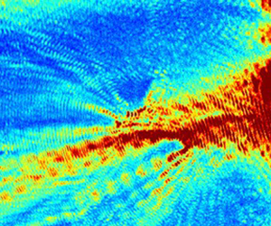
Computation of the bottom pressure field is for the region to the left of the dashed line shown in figure 6. Both the time series of figure 7 and the pressure maps of figure 8 demonstrate agreement between theory and numerics at constant depth (see the pressure field animation in the supplementary materials). Introduction of variable depth leads to the expected discrepancies between theory and the numerical model. However, even in the variable depth case, most of the important physics can be captured using the model. In figure 9, we can see the superposition of pressure signals emanating from multiple slender faults with differing orientations, resulting in areas of high pressure, and areas where the signal is weaker. The pressure contours of column three in figure 8 and the third column of figure 9 highlight the missing processes of refraction, diffraction and interference induced by the variable sea depth and areas of localised elevation (red coloured areas figure 6), with refraction dominating all modes in deep water (Renzi Reference Renzi2017). In figure 6, there is a transect with a seamount located approximately one third of the way along AB. The depth profile for this transect is shown at the top of figure 10. Also shown in figure 10 are pressure signals along the transect for three different times. The variable depth case (red trace) shows attenuation of the signal for points along the transect past 400 km (i.e. just after the seamount). This shadowing effect is also apparent in figure 9 where the seamount is to be found at approximately  $x=-1500$,
  $y=-100$ km. More generally, acoustic–gravity waves propagating into shallow sea depth experience frequency filtering by the water layer (Abdolali et al. Reference Abdolali, Cecioni, Bellotti and Kirby2015a; Cecioni et al. Reference Cecioni, Abdolali, Bellotti and Sammarco2015). Low-order modes are associated with smaller critical depths and are therefore able to propagate further onshore (Abdolali et al. Reference Abdolali, Cecioni, Bellotti and Sammarco2014; Renzi Reference Renzi2017). These results confirm that changing sea depth cannot be ignored when making these calculations, since it affects the timing and scale of the signals measurable at any particular point. For instance, in the placement of hydrophones, the water should be of a depth so as to enable recording of a large frequency range (Abdolali et al. Reference Abdolali, Cecioni, Bellotti and Kirby2015a; Cecioni et al. Reference Cecioni, Abdolali, Bellotti and Sammarco2015).

Figure 6. Overview of area considered for the bottom pressure map. The section to the left of the black dashed line is that used in the calculations for figure 8. The origin of  $x, y$ coordinates is at the earthquake epicentre (yellow star). Fault centroids are shown by blue stars and the faults delineated by rectangles. Depth below sea level is indicated by the colour bar with the white areas at 4 km depth. The four points used to construct the time series of figure 7 are labelled 1, 2, 3 and 4. The transect AB is shown with a dashed line.

Figure 7. (a–d) Dynamic pressure time series for points 1, 2, 3 and 4 (from figure 6). The black trace is the current model (constant depth), the blue trace is a depth-integrated numerical model (constant depth) and the red trace is depth-integrated numerical but with variable depth.

Figure 8. Snapshots of bottom pressure fields at  $t=1260$ s (a–c),
  $t=1800$ s (d–f ) and
  $t=2340$ s (g–i) from the current model, (5.1) (a,d,g), numerical model for the case of constant depth of 4 km (b,e,h) and numerical model for the case of variable depth (c,f ,i). The domain extent is shown in figure 6 and the boundary forcing is imposed along the dashed line – also figure 6. The dynamic pressure variation is indicated with reference to the colour bar where white corresponds to 0 Pa. The transect AB is shown with dashed line in each subplot.

Figure 9. Maximum absolute values of the bottom pressure ( $P$) of the acoustic wave generated by the Sumatra 2004 event during the first 1 h since rupture.


5.2. Displacement function
Aside from linear bottom displacement function (2.4a,b), the sensitivity of surface gravity and acoustic waves are investigated numerically for a half-sine (5.4) and an exponential (5.5) bottom displacement function (shown figure 11(a) (Hammack Reference Hammack1973)):
 \begin{gather} \zeta_s(x,y,t)=\zeta_0\left[\frac{1}{2}\left(1-\cos\frac{{\rm \pi} t}{T}\right)H(T-t)+H(t-T)\right] H(b^2-x^2)H(L^2-y^2) \end{gather}
 \begin{gather}\zeta_e(x,y,t)=\zeta_0(1-\textrm{e}^{-\alpha t})H(b^2-x^2)H(L^2-y^2), \end{gather}
where  $H$ is the Heaviside step function and
  $\zeta _0$ is the residual displacement. For exponential displacement,
  $\zeta _e(t=T)=2\zeta _0/3$ or
  $T=1.11/\alpha$. The linear and exponential displacement functions result in very similar surface elevation plots, whereas their associated acoustic–gravity wave plots show a difference in amplitude, with the exponential displacement function delivering a smaller amplitude. The surface elevation predicted by the current model (general compressible) for a linear displacement function is also shown. The half-sine displacement function shows a marked difference in surface elevation amplitude when compared with either of the linear, or the exponential displacement functions – approximately 50 %. The half-sine displacement function is the only one of the three to have a smooth transition in velocity at
  $t=0$. The amplitude of the acoustic–gravity wave produced in this case ends up larger (by
  $t=1600$ s) than either of the linear or exponential cases, suggesting that energy is directed towards producing a larger acoustic–gravity wave at the expense of the surface wave.

Figure 11. (a) The time series of bottom displacement for linear, half-sine ( $\zeta _s$) and exponential (
 $\zeta _e$) functions. (b) The time series of surface elevation (
 $\eta$) and (c) bottom pressure signals. Coordinates are
  $x= 1000$,
  $y = 0$ km.
6. Discussion
The separation of scales between acoustic and gravity waves indeed suggests analysing each wave type separately, as reported in literature. Such separation allows a comprehensive, but simplified, study compromising the accuracy only slightly. However, such compromise may lead to a twofold negative impact on the implementation of a reliable early tsunami warning system. The first is that reducing the uncertainties is critical in the inverse problem (Bernabe & Usama Reference Bernabe and Usama2021), which can be done with the model without adversely affecting the calculation time. The second is that an inverse approach that employs pure acoustic theory only can initially provide properties of the fault, but then calculations of the rising tsunami need to be carried out. Our model enables simultaneous calculation of all acoustic–gravity modes, including the rising gravity mode (tsunami), thus minimising the calculation time.
The current model includes a constant water-depth assumption, which has implications that cannot be ignored. While the model can estimate the tsunami in the deep water, it may not be effective in describing the propagation over varying bathymetry and the shelf break for two principal reasons. The first lies in the assumption of constant depth, and thus effective techniques that take into account changes due to topography without computing the whole 3-D domain need to be developed. The second reason is the neglect of sea-floor elasticity, which turns out to be important for both tsunami and acoustic–gravity wave arrival times (Kadri Reference Kadri2019). For the tsunami, neglecting elasticity results in overestimation of the phase speed (Watada Reference Watada2013; Watada, Kusumoto & Satake Reference Watada, Kusumoto and Satake2014; Abdolali et al. Reference Abdolali, Kirby and Bellotti2015b, Reference Abdolali, Kadri, Parsons and Kirby2018). The effect is even more dramatic for acoustic–gravity waves as they can couple to the elastic sea floor and travel at speeds reaching  $3900\ \textrm {ms}^{-1}$ which significantly changes their arrival time (Eyov et al. Reference Eyov, Klar, Kadri and Stiassnie2013).
Extensions to the existing model could be developed in many ways, one of which would be to address the assumption of constant sound speed. The work of Michele & Renzi (Reference Michele and Renzi2020) highlighted the importance of including variable sound speed profiles into practical applications such as tsunami early warning. Another area in which the model may be improved lies in the assumption of an idealised rectangular geometry for the faults. Although table 1 of Mei & Kadri (Reference Mei and Kadri2018) shows the rectangular fault assumption to be valid in many cases, it is obviously not valid for all. Future work could include the addition of dip and rake angles as parameters and also provision for the fault to rise with different velocities along its length, rather than the whole fault moving together with one set velocity.
Supplementary material and movies
Supplementary material and movies are available at https://doi.org/10.1017/jfm.2021.101.
Declaration of interests
The authors report no conflict of interest.
Author contributions
U.K. conceptualised the problem B.W. and U.K. derived the theory, A.A. developed the numerical model and B.W. and A.A. performed the simulations. All authors contributed equally to analysing data and reaching conclusions, and in writing the paper.


