


I. INTRODUCTION
Mold slag is a kind of silicate material that is necessary for metallurgical process. During continuous casting, mold flux can not only provide adequate lubrication for solidified shell, but also reduce the horizontal heat transfer to minimize longitudinal cracking (Mills et al., Reference Mills, Fox, Li and Thackray2005). Mold powder added to the top of the mold will be heated by molten steel, and then liquid slag will infiltrate into the gap between steel and solidified shell. On the shell side, mold flux is a thin liquid film that lubricates steel. In the colder region, mold flux solidifies and the solid slag film has an effect on controlling horizontal heat transfer. On the mold side, mold flux exists as a glassy layer due to the high cooling rate. Therefore, solid slag film contains two layers, including a crystalline layer and a glassy layer. Solid slag film, interfacial resistance, and liquid slag film constitute the total thermal resistance between the shell and the mold wall (Cho and Shibata, Reference Cho and Shibata2001; Mills et al., Reference Mills, Fox, Li and Thackray2005).
The interfacial heat resistance accounts for 50% of total thermal resistance. Besides the thickness of the solid slag film, crystalline fraction of the solid slag film is another parameter that affects interfacial heat resistance. With the increase of crystalline fraction, the interfacial heat resistance increases (Cho et al., Reference Cho, Shibata, Emi and Suzuki1998). Therefore, the crystalline fraction of the solid slag film is a key factor to reflect the capability of controlling the horizontal heat transfer. This factor is expected to be kept within a reasonable range, so that the lubrication effect and heat transfer capability of the mold flux can be appropriate for the casting of different kinds of steel (Mills et al., Reference Mills, Courtney, Fox, Harris, Idoyaga and Richardson2002).
Because the crystalline fraction plays an important role on the process control, it is necessary to obtain the quantitative value of crystallinity using an appropriate method. Thermal analysis could provide reliable values for the glass fraction in slag films. However, uncertainties exist in measurements of the glass fraction due to baseline shifts or mechanical collapse of samples (Mills et al., Reference Mills, Fox, Li and Thackray2005). According to studies related to quantitative analysis (Le Blond et al., Reference Le Blond, Cressey, Horwell and Williamson2009; Martin et al., Reference Martin, Beauparlant, Lesage and Tra2012; Fawcett et al., Reference Fawcett, Crowder, Kabekkodu, Needham, Kaduk, Blanton, Petkov, Bucher and Shpanchenko2013), the X-ray diffraction (XRD) method is appropriate to measure the crystallinity of materials. A Rietveld full-pattern fitting method is widely used in quantitative analysis of multicomponent mixtures (Bish and Post, Reference Bish and Post1993). When the observed and calculated standard profiles were used, this method can analyze materials containing imperfect or unknown phases (Taylor and Rui, Reference Taylor and Rui1992). Besides, the Rietveld method can be used for the quantitative determination of crystalline phases in bulk materials (Katsumasa et al., Reference Katsumasa, Yoshitake and Akira1998). Nevertheless, this method could not be applied directly for materials containing amorphous phases, because of difficulties in obtaining Bragg reflection data of amorphous (Ming et al., Reference Ming, Mengqiang, Shuren, Xiaohua, Ting and Song2010). To solve this problem, combination of Rietveld and reference intensity ratio was developed, and the quantitative phase analysis can be performed on glass–ceramic materials (Luisa et al., Reference Luisa, Federica, Isabella, Cristina and Monia2005). These studies indicate that the standard profiles or other references are needed to analyze the amount of each crystalline phase in the materials containing amorphous. Therefore, it is difficult to obtain the crystallinity of the solid slag film directly by the Rietveld method since these materials are always multiphase.
This work aims to obtain crystallinity of materials, and a method of processing diffraction data was developed. This method does not require structure parameters or other references. Computer-generated codes, one for each measured data point, are used to interpret the pattern as to where diffraction peaks exist and what is the angular breadth of each peak's intensity above background. Thus, results can be obtained directly by reading a text file with diffraction data. Values of crystallinity in solid slag films were determined with developed method, and results were compared with values obtained by thermal analysis. Also, factors that may influence calculated results were analyzed and discussed.
II. EXPERIMENTAL
A. Sample preparation
Fifteen slag samples were prepared, and the chemical composition of each slag sample is shown in Table I. M2, M3, M4, and M5 are used in industrial plants, and the chemical compositions of the four samples are analyzed by the X-ray fluorescence (XRF). The other samples were prepared by mixing high purity chemicals. Samples used in industrial plants always contain carbon, lithium oxide, and boron oxide. The amount of these components may not be analyzed accurately. As a result, the total amount of composition for the four samples is not equal to 100.
Table I. Chemical compositions of slag samples (mass%).

B. Solid slag film
Solid slag films were obtained by an HF-200 heat flux simulator in the laboratory (Wen et al., Reference Wen, Tang, Yang and Zhu2012). The schematic of this apparatus and the picture of the solid slag film attached on a copper detector are shown in Figures 1 and 2. Roughly 350 g of prepared slag was put in a graphite crucible and it was heated in a MoSi2 furnace. Temperature was increased to 1400 °C and maintained for about 10 min, so that a homogeneous slag pool could form. Then, cooling water was passed through an alumina tube into the copper detector at a flow rate of 200 L h−1. The temperature of water in and water out was measured by thermocouple placed in the alumina tube. When the copper detector was completely immersed into a mold flux, heat was taken away by moving water, and a solid slag film began to form around the copper detector. After 45 s, the copper detector was taken out of liquid slag and we can get the solid slag film attached on the copper detector, as shown in Figure 2.

Figure 1. Schematic representation of HF-200 heat flux simulator.

Figure 2. Picture of solid slag film.
C. XRD measurement
XRD data were obtained using Rigaku D/Max 2500 PC diffractometer with CuK α radiation. The diffractometer was operated at 40 KV and 150 mA. Intensity data were collected over a 2θ range of 10–90°, with a step interval of 0.02°2θ and counting time of 0.3 s. Soller slits were used in the incident and diffracted beams. M1 slag was chosen to illustrate how to obtain crystallinity by integrated intensities. Samples used in XRD measurements were crushed to grain size of 200 mesh. The composition of M1 slag is shown in Table I. The XRD pattern of M1 slag is shown in Figure 3 [The XRD data files and program used in this paper can be downloaded from http://yun.baidu.com/share/link?shareid=1103912038&uk=528889764].

Figure 3. XRD pattern of M1 slag.
III. DATA ANALYSIS
A. Angle range of diffraction peaks
1. Description of data
There are 4001 data points over the full range of 2θ, and these data points are expressed as A 1, A 2,…, A i , Ai +1,…, A 4001, respectively. For each point, the 2θ angle is expressed as 2θ (A i ), and the diffraction intensity is expressed as I(A i ). When I(A i ) > I(A i+1) and I(A i ) > I(A i−1), A i is expressed as P j . Between P j and P j+1, the point with minimum intensity is expressed as Q k , as shown in Figure 4.

Figure 4. Definition of Δp and Δq.
2. Assigning code for each point
A code will be set for each data point to distinguish data points with different feature. According to criteria listed in Table II, data points can be divided into ten types, and each type has a code. Using the code for each data point, the computer algorithm can then screen for specific profile characteristics such as diffraction peaks due to crystalline phases. Five successive points constitute four connected vectors, as shown in Figure 5. The angle between any two vectors can be expressed as Eq. (1).
 $$\cos \left\langle {\mathop {a} \limits ^{\rightharpoonup}}_i, {\mathop {a} \limits ^{\rightharpoonup}}_j \right\rangle = \displaystyle{{{{\mathop {a} \limits ^{\rightharpoonup}}_i} \cdot {\mathop {a} \limits ^{\rightharpoonup}}_j} \over {\big \vert{\mathop {a} \limits ^{\rightharpoonup}}_i \big \vert \cdot \left \vert{\mathop {a} \limits ^{\rightharpoonup}}_j \right \vert}} \left( {i \ne j} \right)$$
where
 $\left \vert {{\mathop {a} \limits ^{\rightharpoonup}}}_i \right\vert$
and
$\left \vert {{\mathop {a} \limits ^{\rightharpoonup}}}_i \right\vert$
and
 $\left \vert {{\mathop {a} \limits ^{\rightharpoonup}}}_j \right\vert$
are the norm of vectors
$\left \vert {{\mathop {a} \limits ^{\rightharpoonup}}}_j \right\vert$
are the norm of vectors
 ${\mathop{a}\limits^{\rightharpoonup}}_i \, \hbox{and} \, {\mathop{a}\limits^{\rightharpoonup}}_j$
, respectively. When
${\mathop{a}\limits^{\rightharpoonup}}_i \, \hbox{and} \, {\mathop{a}\limits^{\rightharpoonup}}_j$
, respectively. When
 $\cos \langle {\mathop{a}\limits^{\rightharpoonup}}_i, {\mathop{a}\limits^{\rightharpoonup}}_j \rangle $
is higher than 0.75, a straight line can be fitted by plotting I(A
i
) vs. 2θ(A
i
). The codes of the five points were assigned according to the slope of the regression line, as listed in Table II. When cos〈a
i
, aj
〉 is lower than 0.75, the Δp was defined as the difference between I(P
j+1) and I(P
j
), and Δq was defined as the difference between I(Q
k+1) and I(Q
k
). The code of point P
j+1 was assigned according to the value of Δp and Δq, as listed in Table II.
$\cos \langle {\mathop{a}\limits^{\rightharpoonup}}_i, {\mathop{a}\limits^{\rightharpoonup}}_j \rangle $
is higher than 0.75, a straight line can be fitted by plotting I(A
i
) vs. 2θ(A
i
). The codes of the five points were assigned according to the slope of the regression line, as listed in Table II. When cos〈a
i
, aj
〉 is lower than 0.75, the Δp was defined as the difference between I(P
j+1) and I(P
j
), and Δq was defined as the difference between I(Q
k+1) and I(Q
k
). The code of point P
j+1 was assigned according to the value of Δp and Δq, as listed in Table II.

Figure 5. Definition of vectors.
Table II. Codes corresponding to different criteria.

3. Retrieval of diffraction peaks
Four operations were defined before determining the 2θ angle range of each diffraction peak.
-
(1) For data points between A i and A j , the number of points whose corresponding code is C was expressed as NUM(C, A i , Aj );
-
(2) The maximum intensity of point Ai, A i+1, A i+2,… was expressed as max(A i , Ai +1, A i+2,…), while the minimum intensity was expressed as min(A i , Ai +1, A i+2,…);
-
(3) The index of point A i is expressed as &(A i ), and &(A i ) is equal to the difference between 2θ(A i )/0.02 and 499.
The start angle and end angle of a diffraction peak were expressed as 2θ m and 2θ n , respectively, and the method to determine the value of m and n was described with flow charts, as shown in Figures 6 and 7. While the 2θ profile width may not be correct, the codes can still proceed as follows. Three parameters are defined to characterize the shape of the retrieved peaks. Namely, f 1, f 2, and f 3 as defined in Figure 8 describe the symmetry, smoothness and monotonicity of a diffraction peak, respectively. For the three parameters, a weight coefficient was assigned for each parameter, so that the weighted sum of f 1, f 2, and f 3 could be used to evaluate the shape of diffraction peak. The profile is more likely to be a single diffraction peak when the value of parameter f closes to 1, and the method to obtain the value of f is shown in Figure 8. For retrieved peaks with low f(<0.68), adjusting the value of m and n will change the value of parameter f until the maximum is reached, then, the 2θ angle range can be revised.

Figure 6. Flow chart of calculating m.

Figure 7. Flow chart of calculating n.

Figure 8. Flow chart of calculating f.
B. Background subtraction
Cubic spline function fitting was used to obtain background curve because good subsection smoothness could be realized using this method. To get reliable background intensities, the function of fit background in software Jade 5 was used as references to select related threshold values and subsection of cubic spline function (Sarsfield et al., Reference Sarsfield, Davidovich, Desikan, Fakes, Futernik, Hilden, Tan, Yin, Young, Vakkalagadda and Volk2005). In addition, to make calculated results comparable, background intensities of each XRD profile were obtained with the uniform method. For M1 slag, the background intensities I b(2θ i ) at different 2θ are listed in Table III, and the background intensities at any angle could be calculated by interpolation method.
Table III. Background intensities I b (2θ i ) at different 2θ.

C. Calculation of total diffraction intensity I t
After background subtraction, the total diffraction intensities I t can be obtained by integrating intensities from 10 to 90°. This value is equal to the area of the region bounded by the raw XRD profile and the background curve. The value of I t could be expressed as Eq. (2), where I(2θ i ) is the diffraction intensity at 2θ i , and I b(2θ i ) is the background intensity at 2θ i .
 $${I_{\rm t}} = \sum\limits_{i = 1}^{4000} {\displaystyle{{[(I(2{\theta _{i + 1}}) - {I_{\rm b}}(2{\theta _{i + 1}})) + (I(2{\theta _i}) - {I_{\rm b}}(2{\theta _i}))]} \over 2}} \cdot (2{\theta _{i + 1}} - 2{\theta _i})$$
D. Separating the contribution of the amorphous phase
When sample contains both glassy phase and crystalline phase, the total diffraction intensity can be considered as the sum of the intensities due to crystalline phases I c and intensities due to glass I a (Yang et al., Reference Yang, Wen, Quan and Wang2009; Gravier et al., Reference Gravier, Donnadieu, Lay, Doisneau, Bley, Salvo and Blandin2010) [see Eq. (3)]. Obviously, the diffraction intensities due to crystalline phases are superimposed on top of the intensities corresponding to residual amorphous matrix. Separating the contribution of the amorphous phase requires two assumptions:
 $${I_{\rm c}}(2{\theta _i}) = I(2{\theta _i}) - {I_{\rm a}}(2{\theta _i})$$
-
(1) For the amorphous matrix of solid slag film, its XRD pattern is similar to pure glass;
-
(2) The valley of diffraction peak is part of the shape corresponding to amorphous matrix.
For XRD pattern of M1 slag, a “bulge” appears in the range of 20–40°2θ, which can be considered as the contribution of glass in the solid slag film. Outside this range, the intensities of glassy phase are close to background intensities I b. When the 2θ is between 20 and 40°, the values of I a are listed in Table IV.
Table IV. Value of I a when the 2θ is in the range of 20–40°.

E. Evaluation of the diffraction peaks
The structure of crystals in samples is always not perfect. For example, subcrystalline, lattice distortion, and dislocation exist in crystals. Owing to these crystal imperfections, the distribution of diffraction intensity in reciprocal space will be unavoidably influenced, and the shape of diffraction peak will be changed. As a result, the diffraction peak will become wider, and the intensity will decrease. It is difficult to identify perfect crystals in our samples. When these defects in crystals are not very serious, these crystals can be considered as fully crystalline and its corresponding diffraction peak will be used in the calculation. So, the effect of imperfect crystal on diffraction intensities should be taken into consideration, meanwhile, appropriate criterion is necessary to filter diffraction peaks corresponding to fully crystalline. For peaks whose intensities are higher than I a (because of amorphous matrix), two parameters were used to determine whether a diffraction peak is because of complete crystals. The first parameter is the peak value y h (amorphous intensity has been subtracted). This value is equal to the maximum intensity when 2θ is in the range of 2θ m and 2θ n [see Eq. (4)]. The second parameter l [see Eq. (5)] is the ratio of the peak area to the cube of full-width at half-maximum (FWHM). This value is used to describe the degree of diffraction peaks being broadened. The value of parameter l is much higher for sharp diffraction peaks than for broaden peaks.
 $${y_{\rm h}} = \max \left[ {{I_{\rm c}}(2{\theta _m}),{I_{\rm c}}(2{\theta _{m + 1}}),{I_{\rm c}}(2{\theta _{m + 2}}) \cdots {I_{\rm c}}(2{\theta _n})} \right]$$
 $$l = \displaystyle{A \over {{w^3}}}$$
The schematic representation of the two parameters is shown in Figure 9. For a single diffraction peak, the relation between diffraction intensity and angle can be fitted with Gaussian function [see Eq. (6)],
 $$y = {y_0} + \displaystyle{A \over {{w_1} \cdot \sqrt {\pi /2}}} \cdot {e^{ - 2{{(x - {x_{\rm c}})}^2}/w_1^2}} $$
where y represents diffraction intensities; x represents the diffraction angle; y 0 is the baseline of the peak; A is the peak area; w 1 relates to the FWHM of peak [see Eq. (7)]; x c is the horizontal coordinate of the peak point.
 $${w_1} = \displaystyle{w \over {\sqrt {\ln (4)}}} $$

Figure 9. Schematic representation of the two parameters y h .
In Eq. (7), w is the FWHM of peak. For the data point with the highest intensity, its first derivative is equal to zero [see Eq. (8)] and its second derivative [see Eq. (9)] can represent the curvature of peak point.
 $${y^{\prime}}\left( {{x_{\rm c}}} \right) = 0$$
 $${y^{{\prime \prime}}}\left( {x = {x_{\rm c}}} \right) = \displaystyle{{ - 4 \cdot A} \over {\sqrt {\pi /2} \cdot w_1^3}} $$
When the critical values of y
h and l were determined, diffraction peaks corresponding to crystals can be retrieved and percentage of crystalline phase in the solid slag film can be expressed as Eq. (10), where kcry is the crystalline fraction of solid slag film; I
k
is the integration of intensities contributed by complete crystals; I
t is the total diffraction intensity;
 ${I_{\rm c}}(2\theta\, _{\!i}^j )$
is the intensity of the jth peak at 2θ
i
and the subscript “c” means the peak is because of complete crystal.
${I_{\rm c}}(2\theta\, _{\!i}^j )$
is the intensity of the jth peak at 2θ
i
and the subscript “c” means the peak is because of complete crystal.
 $$\eqalign{kcry &= \displaystyle{{{I_k}} \over {{I_t}}} \cr &= \displaystyle{ \matrix{&\sum\nolimits_{\,j = 1}^s \sum\nolimits_{i = m}^n ({I_{\rm c}}(2\theta _i^j ) + ({I_{\rm c}}(2\theta _{i + 1}^j ))/2) \hfill \cr &\quad \times (2\theta _{i + 1}^j - 2\theta _i^j ) \hfill} \over \eqalign{&\sum\nolimits_{i = 1}^{4000} [(I(2{\theta _{i + 1}}) - {I_{\rm b}}(2{\theta _{i + 1}})) + (I(2{\theta _i}) - {I_{\rm b}}(2{\theta _i}))]/2 \cr &\quad \cdot (2{\theta _{i + 1}} - 2{\theta _i})} }} $$
Reference values of crystallinity are needed to determine the critical value of y h and l. Therefore, thermal analysis was used to calculate the crystallinity of solid slag films, and results can help us choose appropriate critical value for the two parameters. When thermal analysis was used (Mills et al., Reference Mills, Courtney, Fox, Harris, Idoyaga and Richardson2002; Yang et al., Reference Yang, Wen, Quan and Wang2009), the crystalline fraction could be expressed as Eq. (11),
 $$kcry{2_{}} = 1 - \displaystyle{{\Delta {H_f}} \over {\Delta {H_a}}}$$
where kcry2 is the crystalline fraction obtained by the DSC method, ΔH f is the enthalpy of solid slag film, ΔH a is the enthalpy of pure glass. In experiment, we have tried our best to keep the cooling rate of liquid slag as high as possible, and crystal has less opportunity to precipitate from liquid slag. For M1 slag, the XRD pattern of quenched slag is shown in Figure 10. From Figure 10, we can see there are very few crystals in quenched slag. So, the quenched slag was used to substitute the glassy phase in the solid slag film, and ΔH a was substituted by the enthalpy of corresponding quenched slag. NETSCH STA 449 Jupiter f3 with flowing purified Ar was used for thermal analysis. Temperature was increased to 1300 °C with a heating rate of 20 °C min−1. The enthalpy of samples was calculated by software NETZSCH Proteus® Thermal Analysis. Results of DSC measurements are listed in Table V. Experimental results show that the crystallinity obtained by the XRD method is very close to reference value when the critical value of y h and l are selected as 100 and 1000, respectively, as shown in Figure 11. This result indicates that the two parameters can be used to character the shape of diffraction peaks. When the value of y h is higher than 100 and the value of l is higher than 1000, a diffraction peak due to complete crystal will be identified. The position of peaks corresponding to crystals is marked in Figure 3. For each peak, the values of several parameters including 2θ m , 2θ n , yh, l, and A are listed in Table VI.

Figure 10. XRD pattern of quenched slag M1.
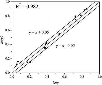
Figure 11. Comparison of calculated results with reference values.
Table V. Crystalline fraction of each solid slag film obtained by DSC method.

Table VI. Values of parameters for M1 slag.

IV. RESULTS AND DISCUSSION
A. Statistics for results of repeated measurements
Considering that random noise in experimental data can have a major impact on peak finding and intensity determination, the impact of counting statistics needs to be discussed. Slag M9 with high crystallinity and slag M11 with low crystallinity were remeasured, and their XRD patterns are shown in Figures 12 and 13, respectively. In Figure 12, the upper XRD pattern (M9-2) is result of second measurement for slag M9. In Figure 13, the upper XRD pattern (M11-2) is the result of second measurement of slag M11. The differences of peak position, peak intensity, and FWHM between two measurements were calculated to discuss how the results vary from each other. For slag M9, the differences of peak position, peak intensity, and FWHM are shown in Figure 14. From statistics of errors in diffraction angle, intensity, and FWHM, the frequency of each parameter in different intervals is listed in Table VII.

Figure 12. Results of repeated measurements for slag M9.

Figure 13. Results of repeated measurements for slag M11.

Figure 14. Differences of peak position, peak intensity, and FWHM for slag M9.
Table VII. Frequency of each parameter in different intervals for slag M9.

For slag M9, 40 diffraction peaks were observed using software Jade 5, and these peaks were also found in the XRD pattern of slag M9-2. From Figures 12 and 13, differences of peak position, peak intensity, and FWHM exist in the two XRD patterns. From Table VII, for most of the peaks, the difference of 2θ between M9 and M9-2 is no more than 0.05. When the value of ∆2θ is higher than 0.15, the difference of 2θ between M9 and M9-2 was considered as large deviations. However, only 10% of peaks are in this range. The statistics of FWHM indicates that for 72.5% of peaks, the difference between M9 and M9-2 ranges from −0.1 to 0.1. From these results, it could be concluded that both the position and shape of diffraction peaks did not change much in the two measurements. In addition, there are 65% of peaks whose values of |∆I| are lower than 50, and no diffraction peak with large deviation (|∆I| > 150) is observed in the two XRD patterns. The crystallinity is 0.728 for M9 and 0.700 for M9-2. These results indicate that the XRD patterns obtained from two measurements are close to each other. As a result, the value of crystallinity obtained from the XRD pattern of M9-2 is also close to the value obtained from the XRD pattern of M9.
For slag M11, the differences of peak position, peak intensity, and FWHM are shown in Figure 15. The frequency of each parameter in different intervals is listed in Table VIII.

Figure 15. Differences of peak position, peak intensity, and FWHM for slag M11.
Table VIII. Frequency of each parameter in different intervals for slag M11

Compared with slag M9, slag M11 has low crystallinity, and the number of diffraction peaks is lower than the number of peaks in the XRD pattern of M9. From Table VIII, for most of the peaks, the difference of 2θ between M11 and M11-2 ranges from −0.05 to 0.05, and there are only six peaks whose values of |∆2θ| are outside this range. For 70% of peaks, the difference of FWHM between M11 and M11-2 ranges from −0.1 to 0.1, which is similar to the statistics of slag M9. These results indicate that the position and shape of peaks have small changes in repeated measurements. It was noted that when the diffraction angle is between 20 and 40°, the intensities of amorphous phase in slag M11-2 are lower than the intensities of amorphous phase in slag M11. Meanwhile, diffraction peaks with large deviations (|∆I| > 150) are observed in the XRD pattern of slag M11, and the frequency is 0.1. In spite of these differences, the crystallinity calculated from the experimental data is close to each other. The values of slag M11 and M11-2 are 0.210 and 0.229, respectively.
From the above discussion, whether for sample with high crystallinity or for sample with low crystallinity, random noise in measurement can influence the position and intensity of diffraction peaks, but this kind of noise has minor effect on calculated results of crystallinity.
B. Results of crystallinity
Background subtraction, separation of amorphous phase, and retrieval of diffraction peaks have been done for each slag sample, and the values of I k , It , and kcry are listed in Table IX. Figure 3 shows a typical XRD pattern of solid slag film. From Figure 3, when 2θ is in the range of 20–40°, a “bulge” was observed on XRD patterns. This trend is particularly obvious on slag films with low crystalline fraction, such as M1, M4, M5, M8, M11, M13, and M14. For slags whose crystalline fraction is higher, diffraction peaks are mainly distributed between 20 and 70°. The number of diffraction peaks is related to the types of crystals, and the diffraction intensity of each peak is related to the volume of unit cell. Obviously, the integration of intensities I k is higher for solid slag films with high crystalline fraction than for slag films with low crystalline fraction. Thus, the crystalline fraction of solid slag film relates to the integration of intensities I k . Using nonlinear fitting, the relation between crystalline fraction and I k can be fitted to an exponential function [see Eq. (12)].
 $$kcry = 0.855 - 0.872 \cdot \exp \left( {\displaystyle{{{I_k}} \over { - {{1853.27}_{}}}}\;} \right)\;\;(2058 \lt {I_k} \lt 7566)$$
Table IX. Values of I k , It , and kcry for the experimental slags.

Equation (12) indicates that approximate value of k cry can be obtained by calculating integrated intensities I k and this value is close to the result calculated from Eq. (10) (see Figure 16).

Figure 16. Value of kcry changing with I k.
The range of 2θ in Eq. (10) is from 10 to 90°. When the integration interval is changed, another result can be obtained. The effect of integration interval on the value of k cry can be investigated using different angle range as integration interval to calculate k cry . Roughly 20 to 45°, 35 to 60°, and 45 to 70° were chosen as three integration intervals, and the value of kcry with respect to each integration interval was calculated using the same method. The values of kcry calculated with different integration intervals are shown in Figures 17–19. Results calculated with three different integration intervals are close to each other, which indicate that the selection of integration interval does not have much effect on results. Furthermore, when the integration interval was selected as 20–45°, calculated results have the highest correlation with results obtained by Eq. (10). Therefore, in order to simplify computations, 20–45° was considered as an appropriate range of 2θ.

Figure 17. Calculated results when 2θ is between 20 and 45°.

Figure 18. Calculated results when 2θ is between 35 and 60°.

Figure 19. Calculated results when 2θ is between 45 and 70°.
From calculated results, the correlation coefficient is higher than 0.9 whatever the integration interval, which indicates that the presented method could be well applied in data processing of the 15 slags. Even so, the number of samples is not large enough to give a comprehensive evaluation for this method. However, the value of crystallinity for experimental slag is between 0.06 and 0.85, and this range is wide enough to cover the crystallinity of conventional slag films. In addition, crystals formed in common slag films exist in the experimental samples, such as cuspidine (3CaO.2SiO2.CaF2), gehlenite (2CaO.SiO2.Al2O3), dicalcium silicate (2CaO.SiO2), and calcium fluoride (CaF2). Therefore, parameters and corresponding values proposed in this work could provide references for most of the slag films, although the crystal type and crystallinity are different for samples with different chemical compositions. Moreover, the value of I k will not be overestimated since two parameters were used to identify diffraction peaks retrieved. Further work will focus on the selection of appropriate parameters and determination of critical values to make this method applicable for more samples and other crystalline materials.
V. CONCLUSION
The crystalline fraction of the solid slag film could be determined using the developed method. A computer program was written in C language, and the diffraction profile was analyzed. The value of crystalline fraction can be obtained directly by reading a text file with raw data. Two parameters, y h and l, could be used to analyze the shape of diffraction peaks, and results calculated based on this analysis are close to reference values.
The crystalline fraction of the solid slag film increases with the increase of integrated intensities corresponding to crystalline phases. The relation between integrated intensities I k and crystallinity of the solid slag film can be expressed using nonlinear fitting; so approximate value of crystalline fraction can be obtained by calculating integrated intensities. Besides, the selection of integration interval does not have much effect on results. To simplify computations, 20–45° was considered as an appropriate integration interval.
SUPPLEMENTARY MATERIAL
The supplementary material for this article can be found at http://dx.doi.org/10.1017/S0885715615000986
ACKNOWLEDGEMENT
The authors express their gratitude to the National Science Foundation (Grant no. 51274260) of China for providing financial support which enabled this study to be successfully carried out.


