INTRODUCTION
The hydrogeological and hydraulic conditions of the Great Hungarian Plain (GHP) are favorable for developing gravitationally controlled regional groundwater flow systems (Erdélyi Reference Erdélyi1976). One of the elevated recharge areas, the Nyírség (NE Hungary) was a deep-lying flat territory that started uplifting about 15,000 years ago in parallel with sinking of boundary zones. This geological event drastically changed the hydrogeological conditions of Nyírség becoming regional recharge area instead of the former discharge area. The main goal of the paper is to present the results of a steady-state groundwater flow model (Székely Reference Székely2006) verification by radiocarbon (14C) data, taking into consideration these paleo-hydrogeological changes. The FS (Flow-Solute) software developed by Székely (Reference Székely1990) was successfully used for modeling the present hydrogeological conditions of the groundwater flow system.
Detailed descriptions of the 14C tool and dating techniques including their restrictions can be found in numerous publications (e.g. Fritz and Fontes Reference Fritz and Fontes1980; Clark and Fritz 1999; Cook and Herczeg Reference Cook and Herczeg2000; International Atomic Energy Agency 2000). Large number of publications using groundwater 14C ages for verification and calibration of conceptual and/or mathematical models indicates their importance. Conceptual groundwater model of GHP (Erdélyi Reference Erdélyi1976) has been verified by previous 14C data (Deák Reference Deák1979; Marton et al. 1980; Marton Reference Marton1981; Dénes and Deák 1981; Deák et al. Reference Deák, Stute, Rudolph and Sonntag1987; Stute and Deák Reference Stute and Deák1989; Szücs et al. Reference Szűcs, Kompár, Palcsu and Deák2015). Groundwater ages in the main aquifer (Lower Quaternary, Q1) of regional recharge areas are less than 10 ka, and gradually grow towards the discharge areas following the decrease of piezometric heads. Mean vertical and lateral flow velocities calculated from groundwater ages are 30–60 mm/a and 2–3 m/a, respectively.
Groundwater mathematical models of two recharge areas of the GHP, the Danube-Tisza interfluvial area (Sanford et al. Reference Sanford, Révész, Deák, Seiler and Wohnlich2001) and the alluvial fan of river Maros (Deák et al. Reference Deák, Deseő and Davidesz1996) have been verified by 14C ages, based on theoretical considerations (IAEA 1996, 2013; Sanford Reference Sanford2011; Salmon et al. Reference Salmon, Prommer, Park, Meredith, Turner and McCallum2015). Calculated 14C groundwater ages agreed well with the modeled ages in both areas, despite uncertainties of dating caused by mixing, dispersion, diffusion, etc. Many of these uncertainties can be reduced by modeling the raw 14C data instead of groundwater ages (Suckow Reference Suckow2014; Siade et al. Reference Siade, Prommer, Suckow and Raiber2018), therefore we modeled 14C content of groundwater and compared to the observed and δ13C corrected 14C data (see section “δ13C Correction of 14C Data”). The numerical FS software of Székely (Reference Székely1990) simulates mixing, adsorption and desorption in addition to radioactive decay (t1/2=5730 a) at modeling of 14C content.
STUDY AREA
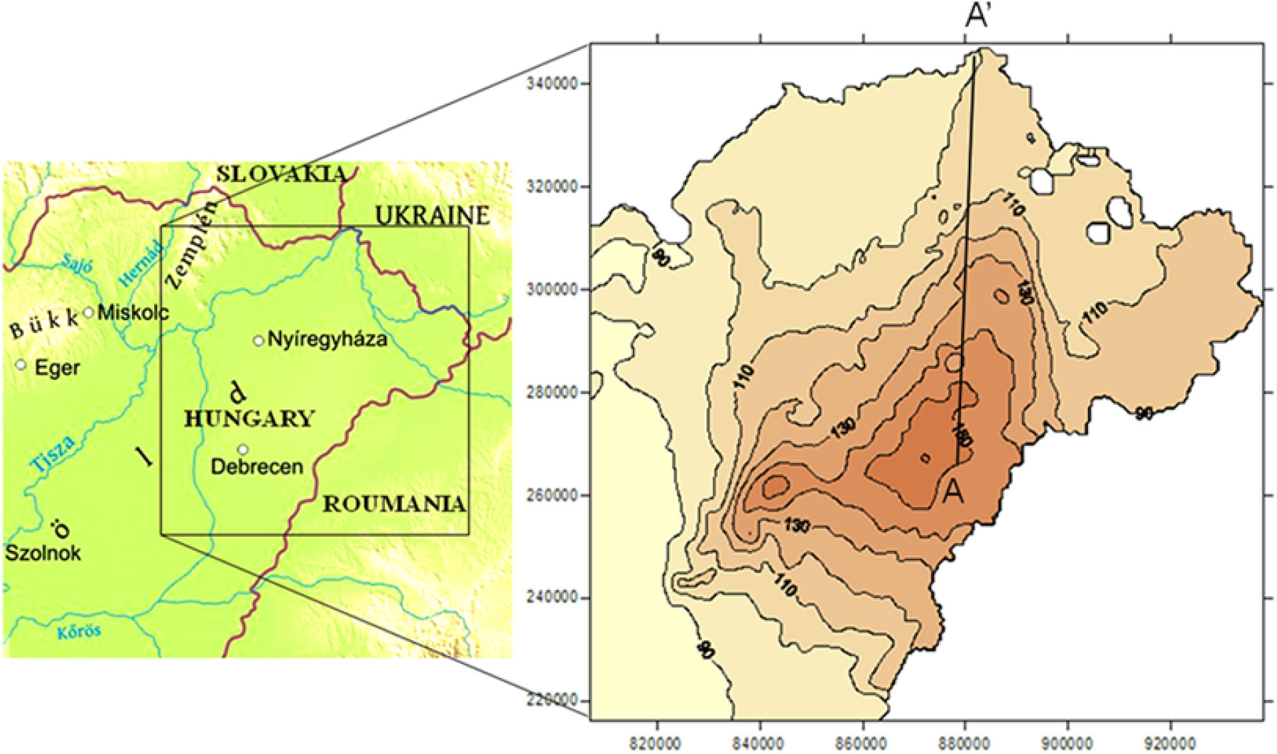
The Great Hungarian Plain is a large sedimentary basin, structurally representing a deep depression formed mainly during the late Tertiary and Quaternary ages. The 132 × 132 km2 square-shaped study area is shown in Figure 1. It occupies the very NE part of the GHP and incorporates the Hungarian part of that geographic unit. This area constitutes the watershed of the Tisza River and its tributaries. Due to neotectonic events, erosion, sufficient deposition of alluvial sediments and windblown sand the originally flat alluvial plain now has a sizeable contrast in land surface elevation. The central part of the area (Nyírség) rose practically 30 m with the margins sinking at a different rate. These tectonic movements started 15 ka ago and caused the present “relief island” character with 150 m average elevation, reaching 183 m above sea level at the highest point.

Figure 1 Location map (left) and shallow groundwater table contours (right) of the study area.
A shallow groundwater table following the top of the porous multi-layered aquifer presents around 80 m difference over the study area (right plot in Figure 1). This head difference acts as the driving force and controls the recharge-discharge, flow as well as the solute transport processes of the porous multi-layered gravitational flow system (Székely et al. Reference Székely, Deák, Szűcs, Kovács, Kompár, Zákányi and Molnár2017). The layered-lenticular porous groundwater flow system is composed of the Quaternary-Pliocene-Upper Pannonian clastic sediments ranging from clay to gravel.
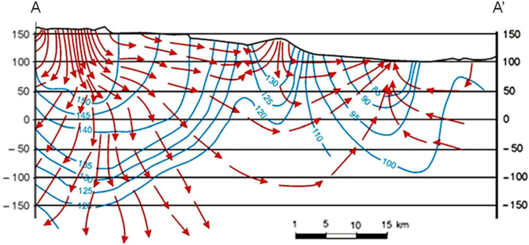
Using the available piezometric head data, Marton et al. (1980) performed flow-net analysis and published the hydrodynamic section showing the equipotential contours along with the associated streamlines. Virág (Reference Virág2013) updated that plot; its northern part is shown in Figure 2. The line A – A’ in Figure 1 marks the path of the cited section.

Figure 2 Vertical section A – A’ showing the equipotential contours and the streamlines (after Virág Reference Virág2013 with the author’s permission).
The blue curves in Figure 2 show the equipotential lines whereas the red arrows mark the flow paths. The plot demonstrates the elevated recharge area with downward seepage on the left-hand side and the flat discharge area with upward groundwater flow on the right-hand side. A minor recharge area is developed also in the middle part of the section. The above sub-domains are connected with transition zones exhibiting predominantly lateral flow.
HYDROSTRATIGRAPHY
The layered-lenticular porous groundwater flow system is composed of the Quaternary-Pliocene-Upper Pannonian clastic sediments ranging from clay to gravel and comprises five model layers. All of these are heterogeneous, layers 2−5 exhibits multi-layered and lenticular structure. Geologic and geophysical logs of 1410 wells were used to delineate the horizontal and vertical boundaries of the model layers (Székely Reference Székely2006).
The first model layer is defined as the uppermost 5 m thick section of the saturated porous formation. The surface of the flow domain is elevated between 80 and 160 m above the sea level and is very similar to the shallow groundwater table shown in Figure 1. The second model layer of maximum thickness 210 m comprises the Upper and Middle Quaternary (Q2-3) sandy-silty sediments. This hydrostratigraphic unit has moderate to low lateral hydraulic conductivity in the lower part and higher value of maximum 18 m/d above.
The third model layer corresponds to the Lower Quaternary (Q1) sandy-gravelly deposits of thickness 0–140 m and maximum lateral hydraulic conductivity of 34 m/d. This section extends to the depth of 330 m and constitutes the main aquifer of the study area. This water-bearing unit is used as the base source of the drinking water supply for large cities, settlements, agricultural and industrial enterprises.
The fourth model layer includes the less-permeable Pliocene (Pl) sediments with the highest lateral hydraulic conductivity of 4 m/d. The maximum thickness and depth to the bottom of this hydrostratigraphic unit are 490 and 710 m, respectively. This model layer is composed of predominantly silty-clayey layers and lenses with the limited appearance of sandy beds.
The fifth model layer incorporates the multi-layered sandy-clayey Upper Pannonian (P2) thermal water aquifer system. This unit of maximum thickness 1330 m and depth 1940 m overlies the consolidated, low permeability Lower Pannonian mostly shale deposits. The lateral hydraulic conductivity of the formation reaches 8 m/d. The thermal water of the P2 model layer is widely used for balneology, recreation and geothermal heating. At present, the deep, consolidated sandstone layers of former gas reservoirs are also utilized for underground gas storage.
The vertical hydraulic conductivity of the model layers decreases with depth from 0.4 to 0.05 m/d. The increase of hydraulic conductivity with the temperature is considered at inflow and transport modeling.
The maps of hydraulic conductivities of model layers with the above maximum values have been constructed via model calibration by fitting the measured and simulated unsteady drawdown over the period 1971–1989 (Székely Reference Székely2006).
GROUNDWATER FLOW MODELING
The transport modeling of radiocarbon (14C) isotope requires groundwater flow modeling to define the flow velocity field responsible for the advective displacement of water and dissolved species. The FS (Flow-Solute) software developed by Székely (Reference Székely1990) was used for modeling the groundwater flow system using Finite Difference scheme. This steady-state groundwater flow model (Székely Reference Székely2006) assumes (1) the previously described hydrostratigraphic model, (2) the shallow groundwater table elevation as the fixed head upper boundary condition, and (3) presumably no-flow lateral boundaries in model layers 2–5. In the present model, the Northern boundary follows the real extension of the porous sediments whereas the Western, Southern and Eastern boundaries are artificial contours or state borders (Szucs et al. Reference Szűcs, Kompár, Palcsu and Deák2015). The latter three assumptions introduce some approximation error in both flow and transport modeling and, thus, cause an increased discrepancy between the simulated and measured 14C Data in those boundary zones (see section “14C and δ13C Data Used in the Model”).
A 500 × 500 m2 square simulation mesh and point centered Finite Difference schemes were applied in modeling of both steady-state flow and solute transport. Hydrogeologic documentation of 1410 wells were utilized for building maps of lateral and vertical hydraulic conductivities (Székely Reference Székely2006). Figure 3 shows the simulated piezometric head in the Lower Quaternary (Q1) aquifer being the source of water samples used for 14C analyses. The gray domain marks the area recharged from the overlying Upper and Middle Quaternary (Q2-3) formation.

Figure 3 Piezometric head distribution in and the vertical recharge area of the Q1 aquifer unit.
It is assumed that the former flat floodplain was gradually converted into the present hydrogeological scheme exhibiting elevated recharge and depleted discharge areas. Based on the available information (Mezősi Reference Mezősi and Rakonczai2011), 15,000 years (15 ka) is accepted as the time to form the present shape of the land surface and water table elevation.
TRANSPORT SIMULATION OF THE RADIOACTIVE TRACER PROPAGATION
Software Validation
The numerical FS (Flow-Solute) software by Székely (Reference Székely1990) uses the Finite Difference method to simulate the following processes: steady-state flow, recharge-discharge, advection, mixing, adsorption, desorption, and radioactive decay. Heterogeneous, multilayered aquifer systems are considered. Prior to field application the package was verified through modeling the 1D radioactive tracer propagation in the homogeneous domain (Székely et al. Reference Székely, Deák, Szűcs and Zákányi2015).
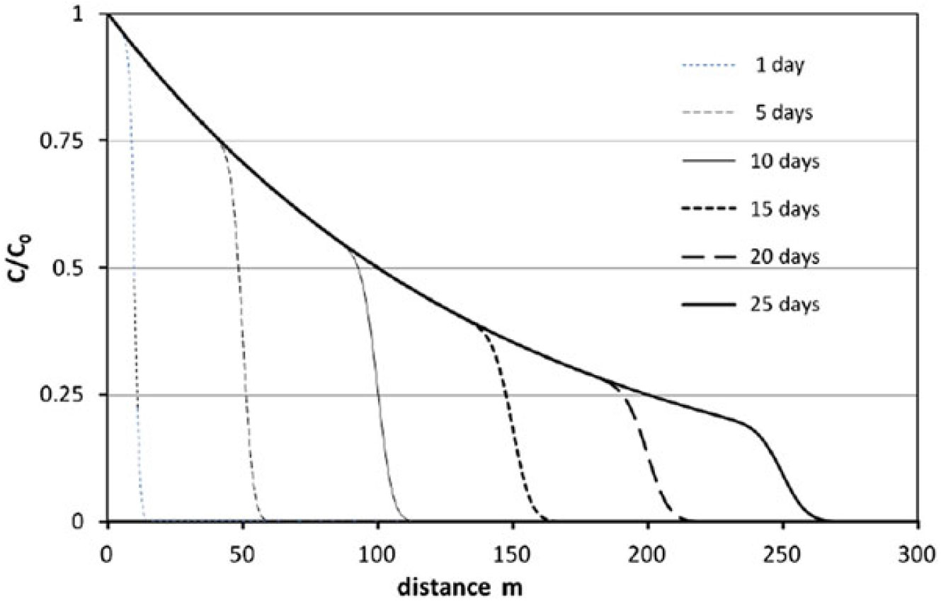
Figure 4 shows the temporal evolution of relative concentration-distance curves of radioactive tracer injected at x = 0 under steady-state flow conditions into a domain containing tracer-free groundwater. The following parameters are used in the numerical FS simulation: C 0 = injected concentration g/m3, C = simulated concentration g/m3, q = 1 m2/d injected flux, n = 0.1 porosity, α = 0.1 m dispersivity, t 1/2 = 10 d half-life of the isotope. The relative concentration data have also been calculated with the analytical method by Van Genuchten (1981 eq. 27). The two datasets show small difference with a relative deviation of 0.12 % for 275 nonzero data at time 25 d.

Figure 4 Numerical transport modeling of the 1D radioactive tracer transport using the FS software (Székely Reference Székely1990).
The verification test shown was also performed for the MODFLOW based GMS software package (AQUAVEO 2013). Among the tested seven solute transport modeling options, the TVD module proved to be appropriate and yielded accurate concentration data for this particular solute transport problem. However, the simulation concluded with higher discrepancy at relative deviation of 0.53%.
Diersch also presented analytical data for a similar transport problem (Diersch Reference Diersch2005, p. 127, Table 10.3). The simulation involved the following parameters: C 0 = 1, q = 0.1 m/d, n = 0.2, α = 5 m, t 1/2 = 40.1 d. The alternate FS simulation showed 0.22 % relative deviation.
Simulation of the Radiocarbon Distribution of the Study Area
Following earlier groundwater isotope studies in the investigated area (Deák Reference Deák1979; Marton et al. 1980; Deák et al. Reference Deák, Stute, Rudolph and Sonntag1987; Stute and Deák Reference Stute and Deák1989), a radiocarbon transport simulation model for the present study area has been developed and verified (Székely et al. Reference Székely, Deák, Szűcs and Zákányi2015). The following assumptions are used in the 14C modeling:
the groundwater flow is steady-state and well described by the used FT model;
the initial 14C concentration of the shallow water table (that is in the first model layer) is 60 pmC;
the half-life of 14C is 5730 years;
due to the assumed stagnant groundwater prior to the 15 ka long transport modeling zero 14C initial concentration is assumed in model layers 2–5;
n = 0.25 porosity and 3D hydrodynamic dispersion are assumed in transport modeling. After manual calibration 200, 20, and 2 m are applied to lateral longitudinal and transversal as well as to vertical dispersivities; and
optimized flow velocity reduction factor should be calculated and used for consideration of the paleo-hydrogeological changes.
The presently prevailing groundwater flow velocity represents the final stage of the land surface evolution exhibiting the maximum difference in land surface elevation. The head difference over the accepted 15-ka-long simulation time was less than the present one causing lower flow velocities in the past. Thus, the time-averaged groundwater flow velocity can be estimated by means of reduction of the current values. This reduction considers the gradual (not necessarily continuous and linear) rise of the water table from the initial flat shape to the present surface exhibiting a head difference of 80 m. Assuming a linear rise of the water table this correction factor should be 0.5. The lack of available geological information about the temporality of rising necessitated calculating the flow reduction factor by using “trial and error” method. In the course of this process, the areal distributions of 14C content in Q1 aquifer were modeled in cases of different flow velocity reduction factors and compared to the measured 14C data.
The best fit between the simulated and measured 14C data was provided at flow velocity reduction factor of 0.4, optimizing the temporal development of flow dynamics. As a result, the number of fitting 14C data increased to 25. This factor is used in the further investigations.
Measured and δ13C Corrected 14C Data in the Lower Quaternary (Q1) Aquifer
In this paper, the14C content data are given aspmC (percent of modern Carbon) as 100 pmC = 13.56 dpm/gC = 0.226 Bq/gC. δ13C data are given as R ratios of 13C/12C related to V-PDB =Vienna-Pee Dee Belemnite standard: δ13C=(Rsample–RV-PDB)/RV-PDB × 1000 [‰].
Detailed previous isotope studies in the modeled area (Deák Reference Deák1979; Marton et al. 1980; Dénes and Deák 1981; Deák et al. Reference Deák, Stute, Rudolph and Sonntag1987; Stute and Deák Reference Stute and Deák1989; VITUKI Reference Deák1995) which produced 14C and δ13C data are supplemented with recent isotope analyses (Székely et al. Reference Székely, Deák, Szűcs and Zákányi2015) listed in Table 1.
Table 1 Measured and simulated 14C data used for the verification of transport modeling.*

* The code number of the data source in the table refers to the following publications and reports listed: (1) Marton et al. 1980; (2) Dénes and Deák 1981; (3) Deák et al. Reference Deák, Stute, Rudolph and Sonntag1987; (4) Marton Reference Marton1981; (5) Deák Reference Deák1995; (6) Székely et al. Reference Székely, Deák, Szűcs and Zákányi2015.
Sampling and Isotope Analysis of Groundwater Samples
The 14C and δ13C data of 32 wells in the model area were collected from different sources thus the sampling and isotope analytical methods have been also different. These methods are listed below referring to the code number of the source of data in Table 1:
no.1 14C data were analyzed in BVFA Arsenal laboratory in Vienna using benzene synthesis and LSC. δ13C data were measured by MS;
no.2 14C data were analyzed in VITUKI (Water Resources Research Centre) laboratory in Budapest using benzene synthesis and LSC. δ13C data were measured in KBFI (Institute of Mining Development), Budapest with MS;
no.3 and no.5 data were analyzed in the laboratory of University of Heidelberg (Germany), using proportional gas counter and MS;
no.4 data were analyzed in the laboratory of ATOMKI (Institute for Nuclear Research, Hungarian Academy of Sciences, Debrecen) using proportional gas counter and MS; and
no.6 samples were analyzed in the ATOMKI using AMS and laser spectrometer.
The earlier samples (no.1 to no.5) for 14C and δ13C analysis were taken from 60 to 120 L of groundwater, precipitating TDIC as BaCO3 by adding NaOH and BaCl2. Recent samples (no.6) were taken from 1 L of groundwater according to the IAEA Guideline (IAEA Sampling booklet) for sampling.
Standard deviations of 14C analysis can be found in Table 1. Accuracy of the δ13C data is ± 0.2 ‰.
δ13C Correction of 14C Data
The initial 14C content of groundwater at the infiltration was assumed to be A0 = 60 pmC in the transport model. This is an average value, but our previous investigations (Deák Reference Deák1979; Stute and Deák 1987) showed that A0 values are not uniform depending on the recharge conditions. The main source of 14C in groundwater is dilution of soil zone CO2 by dissolution of carbonate minerals at infiltration: CaCO3 + CO2 + H2O → Ca2+ + 2HCO3 -. The atmospheric 14C content is, by convention, 100 pmC (at the infiltration of very old groundwater i.e. before nuclear-bomb tests), while 14C content of very old soil carbonate minerals is 0 pmC. Pearson’s equation (Pearson Reference Pearson1965) is generally used to calculate A0 using stable carbon isotope ratio (δ13C) values:
 $${{\rm{A}}_0} = {{\left( {{{\rm{\delta }}^{13}}{{\rm{C}}_{{\rm{measured}}}} - {{\rm{\delta }}^{13}}{{\rm{C}}_{{\rm{carbonate}}}}} \right)} \over {\left( {{{\rm{\delta }}^{13}}{{\rm{C}}_{{\rm{CO}}2}} - {{\rm{\delta }}^{13}}{{\rm{C}}_{{\rm{carbonate}}}}} \right)}} \times 100{\rm{}}\left[ {{\rm{pmC}}} \right]$$
We assume δ13Ccarbonate = 0‰ and δ13CCO2 = -25‰. A0 = 60 pmC initial 14C content means -15‰ initial δ13C ratio by Pearson’s equation. The measured 14C data listed in Table 1 are corrected for A0 = 60 pmC using the equation: Acorr = Ameas × (–15‰ / δ13Cmeas).
Although the main driver of 14C decrease along groundwater flow paths is radioactive decay (t1/2 = 5730 years) but chemical processes generally excess TDIC can also alter the 14C content. Fortunately, these non-radioactive decreases can be controlled by the stable carbon isotope ratio (δ13C) values. Accepting δ13C = 0‰ for the excess TDIC, Pearson’s equation also takes the effect of the excess TDIC into consideration.
Table 1 presents the measured and δ13C corrected (Acorr) 14C values of 32 groundwater samples taken from the Q1 aquifer. The δ13C data of three wells were not available therefore the measured 14C values were accepted as corrected data.
14C and δ13C Data Used in the Model
Available 14C and δ13C data of 32 groundwater samples from Q1 aquifer are listed in Table 1.
Comparison of Simulated and Corrected 14C Data of Groundwater in the Q1 Aquifer
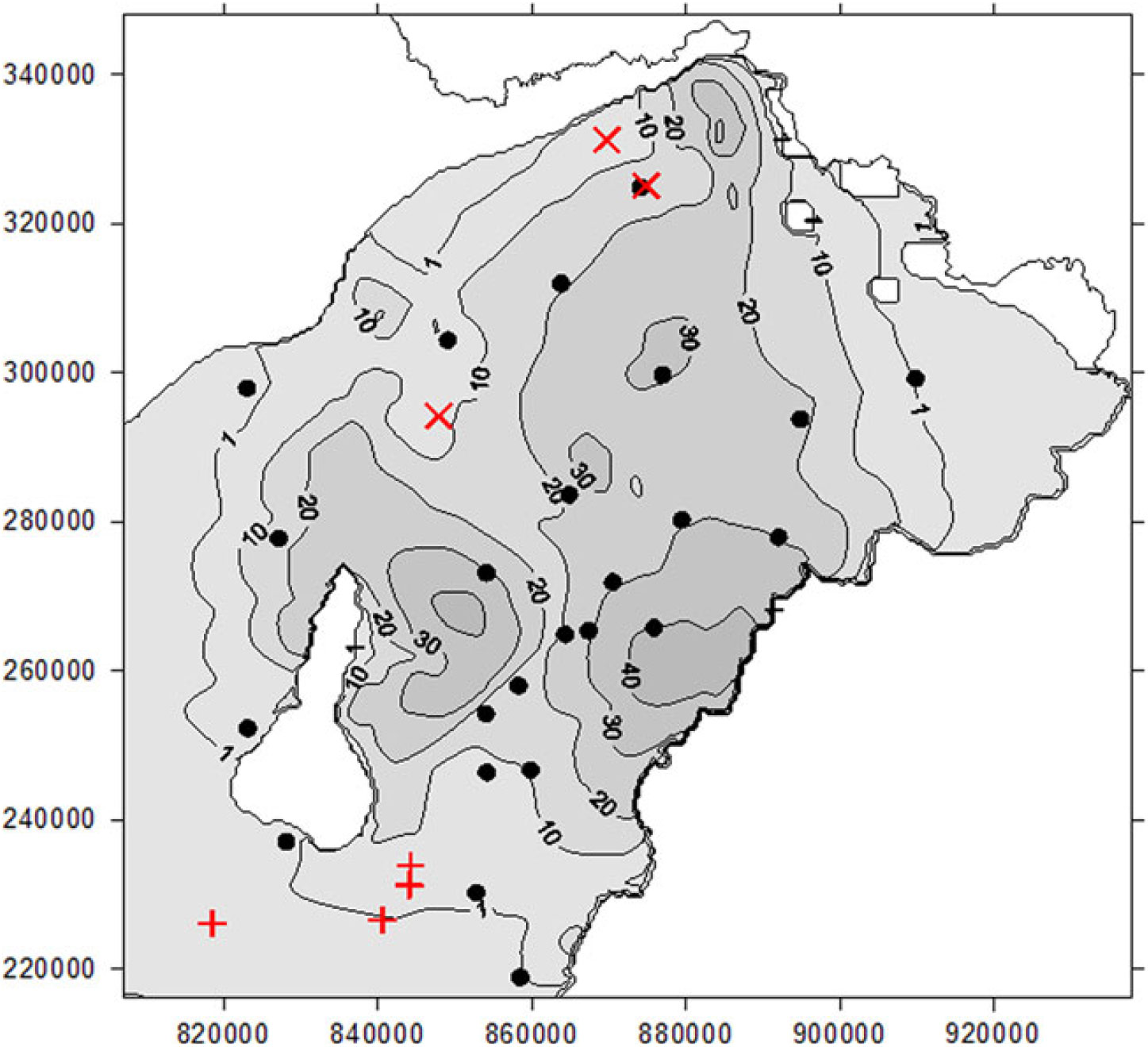
Figure 5 shows the simulated 14C concentration and the water sampling locations at the middle depth of the Lower Quaternary model layer no.3, using flow velocity reduction factor of 0.4. As indicated before, this unit (Q1) constitutes the main aquifer of the area. Also, most of the radiocarbon measurements are performed on water samples obtained from this sandy-gravelly section.

Figure 5 Simulated contour lines of the mean 14C activity (pmC) and the results of comparison with corrected 14C data in the Q1 aquifer.
The simulated 14C data show considerable vertical variation between and within the model layers. Therefore, the measured data are compared with the fitting interval bounded with the concentrations calculated for the top and the bottom of the Q1 aquifer unit. The latter values are defined by means of vertical interpolation of the 14C pmC data simulated in over- and underlying model layers. The use of such a fitting interval helps to reduce the interpretation problem caused by the uncertain sampling depth from wells and the effect of long and/or discontinuous screening. The latter wells yield mixed water pumped from various depth intervals screened in wells under consideration.
Three categories of measured data are encountered (see Figure 5). Corrected 14C data fitting to the simulated interval are marked with circles. These data constitute 78% of the 32 measurements. The symbols + and × refer to measured and corrected 14C data found above (overshoot) and below (undershoot) the simulated intervals, respectively.
The three undershooting data (i.e. measurements below the expected interval) may be associated with local lithological, structural or hydrogeological disturbances of the underlying Pliocene formation carrying groundwater of very low, practically zero 14C content.
Demeter et al. (Reference Demeter, Püspöki, Lazányi and Buday2010) performed a sequence stratigraphic analysis of the Quaternary deposits in the Nyíregyháza-Szatmárnémeti area. The authors found sharp, irregular heterogeneity in the layered-lenticular, sandy-silty-clayey formation. At some locations where the sandy lenses are embedded into larger clayey bodies lithologically based stagnant zones may develop. Samples from such trapped water source usually exhibit exceptionally low 14C activity.
The four overshooting data may be related to either (1) the increased downward seepage of the groundwater at the waterworks due to the sufficient (several 10 m) local drawdowns induced by over-exploitation in the past decades or (2) Western, Southern, and Eastern boundaries in models are artificial contours or the state border causing an increased discrepancy between the simulated and measured 14C data in those boundary zones, or (3) the uplifting of the Nyírség area had been starting earlier than it was assumed in the modeling. In the latter case, the infiltration and the extrusion of the older groundwater could be started earlier, thus the 14C containing groundwater could get farther and deeper from the recharge area. These hypotheses need further verification.
CONCLUSIONS
The results emphasize the importance of the joint application of modeling and natural tracer methods interdependently supporting the reliability of both techniques (Szucs et al. Reference Szucs, Civan and Virag2006) even in such a complex hydrogeological environment (paleo-hydrogeology). The measured and δ13C corrected 14C groundwater data served as a solid base to find the most appropriate groundwater flow velocity factor (0.4). Applying this flow velocity correction, 78% of the measured and δ13C corrected 14C data are within the interval simulated at the top and the bottom of the Lower Quaternary layer, validating the applied model. Additionally, the comparison of measured and simulated 14C data draw attention to other hydrogeological effects that need further investigations.
Overshooting data can be found in the southwestern part of the area. Here the presence of original pre-lifting groundwater was predicted with 0 pmC 14C content but 1–3 pmC were measured. The possible reasons of these differences are (1) the original pre-uplift 14C content of groundwater was not 0 pmC or (2) the area is not closed in the southwestern direction as accepted as a boundary condition in modeling. Undershooting 14C data may be associated with (1) local lithological, structural or hydrogeological disturbances of the underlying Pliocene formation carrying groundwater of lower 14C content or (2) local stagnant zones based on sandy lenses embedded into larger clayey bodies.
The results obtained clearly indicate that the applied steady-state model assuming 0.4 flow velocity reduction factor is capable to reproduce the observed 14C data in spite of the significant changes of groundwater flow conditions in the last 15 ka in NE Hungary. Further investigations are recommended to extend the analysis to the flow system beyond the state border with Romania and Ukraine.
ACKNOWLEDGMENTS
The research was carried out in the framework of the GINOP-2.3.2-15-2016-00010 “Development of enhanced engineering methods with the aim at utilization of subterranean energy resources” project of the Research Institute of Applied Earth Sciences of the University of Miskolc in the framework of the Széchenyi 2020 Plan, funded by the European Union, co-financed by the European Structural and Investment Funds.