


1 Introduction
For a long time, the influence of roughness elements on the transition from laminar to turbulent flows in airfoils has been a concern for designing airfoils (Jacobs Reference Jacobs1939). In the early 40s Tani & Hama (Reference Tani and Hama1940) and Fage (Reference Fage1943) performed the first wind tunnel investigations devoted to this topic. Yet, roughness induced transition is an important research topic with several open questions.
Both two- and three-dimensional roughness elements have been considered. For two-dimensional roughness elements immersed in two-dimensional boundary layers, Klebanoff & Tidstrom (Reference Klebanoff and Tidstrom1972) show a gradual movement of the transition towards the roughness location with an increase of the roughness Reynolds number (
 $Re_{h}=u_{h}h/\unicode[STIX]{x1D708}$
, where
$Re_{h}=u_{h}h/\unicode[STIX]{x1D708}$
, where
 $h$
is the roughness height,
$h$
is the roughness height,
 $u_{h}$
is the velocity at the roughness top edge and
$u_{h}$
is the velocity at the roughness top edge and
 $\unicode[STIX]{x1D708}$
is the kinematic viscosity). According to Klebanoff & Tidstrom (Reference Klebanoff and Tidstrom1972), Dovgal & Kozlov (Reference Dovgal, Kozlov, Arnal and Michel1990) and Morkovin (Reference Morkovin, Hussaini and Voigt1990) the mean flow distortion in the wake of the roughness induces a rapid amplification of ‘natural’ disturbances present in the boundary layer. Morkovin (Reference Morkovin, Hussaini and Voigt1990) suggests a similarity with the mechanism of long separation bubbles.
$\unicode[STIX]{x1D708}$
is the kinematic viscosity). According to Klebanoff & Tidstrom (Reference Klebanoff and Tidstrom1972), Dovgal & Kozlov (Reference Dovgal, Kozlov, Arnal and Michel1990) and Morkovin (Reference Morkovin, Hussaini and Voigt1990) the mean flow distortion in the wake of the roughness induces a rapid amplification of ‘natural’ disturbances present in the boundary layer. Morkovin (Reference Morkovin, Hussaini and Voigt1990) suggests a similarity with the mechanism of long separation bubbles.
The phenomenon appears more complex for three-dimensional isolated roughness elements. In this case a rapid movement of the transition location towards the roughness is reported by Dryden (Reference Dryden1953), Klebanoff, Schubauer & Tidstrom (Reference Klebanoff, Schubauer and Tidstrom1954), Tani (Reference Tani1961), Tani (Reference Tani1969), Klebanoff, Cleveland & Tidstrom (Reference Klebanoff, Cleveland and Tidstrom1992) and many others, for heights approaching a critical value at which transition would be located at the roughness. Dryden (Reference Dryden1953), Tani (Reference Tani1961) and Tani (Reference Tani1969) develop an empirical correlation for such critical roughness height, based on a critical roughness Reynolds number (
 $Re_{h-Cr}$
). According to Klebanoff et al. (Reference Klebanoff, Schubauer and Tidstrom1954), the critical heights for three-dimensional (3-D) roughness are typically large, of the order of the boundary layer displacement thickness (
$Re_{h-Cr}$
). According to Klebanoff et al. (Reference Klebanoff, Schubauer and Tidstrom1954), the critical heights for three-dimensional (3-D) roughness are typically large, of the order of the boundary layer displacement thickness (
 $\unicode[STIX]{x1D6FF}^{\ast }$
). In the words of Tulio & Sandham (Reference Tulio and Sandham2015) ‘the lack of understanding about mechanisms involved in the transition induced by roughness means that current prediction methodologies still rely upon empirical tools’, and there is concern that better tools are needed. In fact, the empirical correlations aforementioned, in general, do not account for the effect of roughness elements shorter than the critical value. The current work is concerned with this subcritical regime.
$\unicode[STIX]{x1D6FF}^{\ast }$
). In the words of Tulio & Sandham (Reference Tulio and Sandham2015) ‘the lack of understanding about mechanisms involved in the transition induced by roughness means that current prediction methodologies still rely upon empirical tools’, and there is concern that better tools are needed. In fact, the empirical correlations aforementioned, in general, do not account for the effect of roughness elements shorter than the critical value. The current work is concerned with this subcritical regime.
Plogmann, Würz & Krämer (Reference Plogmann, Würz and Krämer2014) present an extensive and detailed review about roughness-induced transition. According to this work, the complexity in the wake of the roughness is a key aspect affecting the transition. They didactically separate the roughness studies into three different categories, namely (i) low, (ii) medium and (iii) high roughness height. Here the same classification is adopted.
For low roughness elements (i), with
 $Re_{h}$
smaller than approximately 5, distortions induced by the excrescence in the mean flow are rather small and consequently vortical structures associated with the roughness are either absent or negligible (Gaster, Grosch & Jackson Reference Gaster, Grosch and Jackson1994). Within this range, the conversion of other disturbances, such as sound waves and free stream vorticity, into Tollmien–Schlichting (TS) waves (referred to as receptivity) is said to be the most prominent mechanism (see Kachanov (Reference Kachanov2000), Saric, Reed & Kerschen (Reference Saric, Reed and Kerschen2002) and Würz et al. (Reference Würz, Herr, Wörner, Rist, Wagner and Kachanov2003) for a review). Contribution of low roughness to transition is usually estimated by transfer functions of this conversion. Saric, Hoos & Radeztsky (Reference Saric, Hoos, Radeztsky, Reda, Reed and Kobayashi1991) report about a receptivity study on a two-dimensional roughness to sound. They show a linear variation of TS response with roughness height, over the range of
$Re_{h}$
smaller than approximately 5, distortions induced by the excrescence in the mean flow are rather small and consequently vortical structures associated with the roughness are either absent or negligible (Gaster, Grosch & Jackson Reference Gaster, Grosch and Jackson1994). Within this range, the conversion of other disturbances, such as sound waves and free stream vorticity, into Tollmien–Schlichting (TS) waves (referred to as receptivity) is said to be the most prominent mechanism (see Kachanov (Reference Kachanov2000), Saric, Reed & Kerschen (Reference Saric, Reed and Kerschen2002) and Würz et al. (Reference Würz, Herr, Wörner, Rist, Wagner and Kachanov2003) for a review). Contribution of low roughness to transition is usually estimated by transfer functions of this conversion. Saric, Hoos & Radeztsky (Reference Saric, Hoos, Radeztsky, Reda, Reed and Kobayashi1991) report about a receptivity study on a two-dimensional roughness to sound. They show a linear variation of TS response with roughness height, over the range of
 $Re_{h}=[0.5;5.0]$
. Later Saric et al. (Reference Saric, Reed and Kerschen2002) revisited the problem and established that the receptivity at two-dimensional roughness departs from linear behaviour for values of
$Re_{h}=[0.5;5.0]$
. Later Saric et al. (Reference Saric, Reed and Kerschen2002) revisited the problem and established that the receptivity at two-dimensional roughness departs from linear behaviour for values of
 $Re_{h}$
above 10. Würz et al. (Reference Würz, Herr, Wörner, Rist, Wagner and Kachanov2003) measure linear transfer function coefficients for acoustic receptivity at a three-dimensional roughness. No information is found about limiting values of
$Re_{h}$
above 10. Würz et al. (Reference Würz, Herr, Wörner, Rist, Wagner and Kachanov2003) measure linear transfer function coefficients for acoustic receptivity at a three-dimensional roughness. No information is found about limiting values of
 $Re_{h}$
for a linear behaviour of receptivity for three-dimensional roughness.
$Re_{h}$
for a linear behaviour of receptivity for three-dimensional roughness.
For medium roughness heights (ii), receptivity can become nonlinear with respect to the roughness height (Saric et al. Reference Saric, Reed and Kerschen2002). In addition, vortical structures develop, as shown in the flow visualizations of Tani (Reference Tani1961), Tobak & Peake (Reference Tobak and Peake1982) and Legendre & Werlé (Reference Legendre and Werlé2001). Kendall (Reference Kendall1981) and Gaster et al. (Reference Gaster, Grosch and Jackson1994) measured the mean flow distortion in the roughness wake using hot-wire anemometry. They observed a velocity deficit in the centreline region downstream of the roughness and streaks of velocity excess on either side. The pattern of mean flow distortion is consistent with the structure of vortices observed in the flow visualizations. However, according to Gaster et al. (Reference Gaster, Grosch and Jackson1994), the strength of the vortical structures is small and they are eventually damped further downstream without affecting the transition. These results confirm earlier observations of Dryden (Reference Dryden1953), Klebanoff et al. (Reference Klebanoff, Schubauer and Tidstrom1954) and Tani (Reference Tani1961). Yet in the literature, no detailed information is given about the effect that these weak steady disturbances could have on the stability of TS waves.
Flow visualizations of Gregory & Walker (Reference Gregory and Walker1956), Mochizuki (Reference Mochizuki1961) and Legendre & Werlé (Reference Legendre and Werlé2001), in the third range of roughness heights (iii), show a rather complex vortical structure in the roughness wake. The critical roughness height above discussed is within this regime. Klebanoff et al. (Reference Klebanoff, Cleveland and Tidstrom1992) associate transition with the unstable behaviour of these vortical structures. However, the mechanism responsible for a rapid amplification of disturbances is not clearly identified. Acarlar & Smith (Reference Acarlar and Smith1992) and Klebanoff et al. (Reference Klebanoff, Cleveland and Tidstrom1992) present detailed investigations of transition induced by roughness having heights close to the boundary layer displacement thickness or larger. Those works highlight two inflection points in the mean flow profiles in the roughness wake as potential sources of flow destabilization. Ergin & White (Reference Ergin and White2006) revisit the problem to show more detailed measurements focusing on the regions of the inflectional base flow. Those results show a coincidence between regions of high inflection and the position of maximum growth of disturbances. They associate this phenomenon with a Kelvin–Helmholtz instability. Bernardini et al. (Reference Bernardini, Pirozzoli, Orlandi and Lele2014), Kegerise et al. (Reference Kegerise, King, Choudhari, Li and Norris2014) and Tulio & Sandham (Reference Tulio and Sandham2015) addressed the problem of excrescences having heights of the order of
 $1.5\unicode[STIX]{x1D6FF}^{\ast }$
(or
$1.5\unicode[STIX]{x1D6FF}^{\ast }$
(or
 ${\approx}0.5\unicode[STIX]{x1D6FF}$
for a flat plate boundary layer) for high-speed flows. According to their results, the phenomena observed at high Mach numbers display many similarities with low-speed cases. Another interesting feature associated with high roughness elements is that under particular circumstances they can delay transition. Cossu & Brandt (Reference Cossu and Brandt2004) and Fransson et al. (Reference Fransson, Brandt, Talamelli and Cossu2005) clearly show TS wave suppression induced by longitudinal streaks in the wake of an array of roughness elements. Those works describe optimal arrangements of high roughness elements which can lead to strong suppression of TS waves.
${\approx}0.5\unicode[STIX]{x1D6FF}$
for a flat plate boundary layer) for high-speed flows. According to their results, the phenomena observed at high Mach numbers display many similarities with low-speed cases. Another interesting feature associated with high roughness elements is that under particular circumstances they can delay transition. Cossu & Brandt (Reference Cossu and Brandt2004) and Fransson et al. (Reference Fransson, Brandt, Talamelli and Cossu2005) clearly show TS wave suppression induced by longitudinal streaks in the wake of an array of roughness elements. Those works describe optimal arrangements of high roughness elements which can lead to strong suppression of TS waves.
The investigation of roughness induced transition in a ‘quiet’ boundary layer is an important topic. However, there is also the situation where the disturbances enter the boundary layer upstream of the roughness. In this latter scenario, interactions between roughness and boundary layer disturbances can be relevant for transition. According to Crouch & Ng (Reference Crouch and Ng2000), Plogmann et al. (Reference Plogmann, Würz and Krämer2014) this corresponds to a more practical case of airfoil boundary layers. At the leading edge, strong variation in the surface curvature can efficiently promote receptivity which introduces disturbances in the boundary layer. If the surface is imperfect, one can expect interactions of TS waves with surface roughness. The current work focus this scenario.
According to Ustinov (Reference Ustinov1995), Crouch (Reference Crouch1997), Rist & Jäger (Reference Rist and Jäger2004), Wang (Reference Wang2004), Wu & Hogg (Reference Wu and Hogg2006) and de Paula, Medeiros & Würz (Reference de Paula, Medeiros and Würz2008) the scattering of a two-dimensional wave at a low three-dimensional hump can excite oblique waves at the same frequency of the incoming TS wave. Crouch (Reference Crouch1997) calculates transfer functions for the wave scattering at an array of low roughness elements (
 $h<0.05\unicode[STIX]{x1D6FF}^{\ast }$
), periodically spaced in the spanwise direction. The results account for nonlinearity related to the amplitude of the waves, but not to the roughness height. Wang (Reference Wang2004) and Plogmann et al. (Reference Plogmann, Würz and Krämer2014) experimentally investigate the interaction of a two-dimensional TS wave with a single three-dimensional roughness of medium height. Their findings show that, depending on the background disturbance level, roughness elements with Reynolds numbers far below the critical for the quiet boundary layer scenario can influence transition. Plogmann et al. (Reference Plogmann, Würz and Krämer2014) focus on the problem of roughness at the leading edge and accordingly describe interactions of medium sized roughness elements with TS waves having small amplitudes.
$h<0.05\unicode[STIX]{x1D6FF}^{\ast }$
), periodically spaced in the spanwise direction. The results account for nonlinearity related to the amplitude of the waves, but not to the roughness height. Wang (Reference Wang2004) and Plogmann et al. (Reference Plogmann, Würz and Krämer2014) experimentally investigate the interaction of a two-dimensional TS wave with a single three-dimensional roughness of medium height. Their findings show that, depending on the background disturbance level, roughness elements with Reynolds numbers far below the critical for the quiet boundary layer scenario can influence transition. Plogmann et al. (Reference Plogmann, Würz and Krämer2014) focus on the problem of roughness at the leading edge and accordingly describe interactions of medium sized roughness elements with TS waves having small amplitudes.
In view of the current state of affairs it appeared that further work would be of interest in the ‘non-quiet’ boundary layer scenario of roughness induced transition. Some of the gaps could be addressed by investigating a combination between a number of wave parameters with a wide range of roughness heights, in a simple base flow condition. For instance, in a case with low roughness height and small TS wave amplitude, interactions are expected to lead to a regime linear with respect to roughness height. Within this regime a linear transfer function between the incoming 2-D TS wave and the outgoing 3-D TS wave could be established. For other combinations of wave and roughness parameters, the range of validity of this linear correlation could be defined. Perhaps, weakly nonlinear corrections for the transfer functions could be experimentally obtained, for which an extended validity range could also be determined. The study would allow also an assessment of possible effects that the mean flow distortion produced by the roughness could have on the wave scattering as well as on the subsequent wave evolution. Influence of TS amplitude and frequency could also be evaluated. To this end, in the current work, the evolution of the waves ensuing from the roughness is studied experimentally under strictly controlled conditions. Analysis of experimental results is assisted by nonlinear parabolized stability equations (PSE) calculations and results are reported accordingly.
The manuscript is organized as follows. After this introduction, the experimental set-up and the methodology are described (for a more detailed description see de Paula et al. (Reference de Paula, Medeiros and Würz2008)). Following, the design of the experiment, the selection of experimental parameters for the investigation are addressed. Then, in § 3, the issue of possible effects that the roughness wake could have on the evolution of the wave system leaving the roughness is investigated. Next, transfer functions for wave scattering at the roughness are estimated. In addition, limiting conditions for linear scattering behaviour are defined. Finally, weakly nonlinear corrections are proposed and model predictions are assessed. In the last section, main conclusions from the work are summarized and discussed.
2 Methodology
2.1 Experimental set-up and procedures
The experiments were carried out in the Laminar Wind Tunnel (LWT) (Wortmann & Althaus Reference Wortmann and Althaus1964) of the University of Stuttgart. It is an open return tunnel with a rectangular test section, which has a cross-sectional area of
 $0.73\times 2.73~\text{m}^{2}$
. For a speed of
$0.73\times 2.73~\text{m}^{2}$
. For a speed of
 $30~\text{m}~\text{s}^{-1}$
, the free stream turbulence level of the flow in the test section is lower than 0.02 % of
$30~\text{m}~\text{s}^{-1}$
, the free stream turbulence level of the flow in the test section is lower than 0.02 % of
 $U_{\infty }$
in the range of 20–5000 Hz.
$U_{\infty }$
in the range of 20–5000 Hz.

Figure 1. Experimental set-up.
The experiments are performed on an airfoil model with a 600 mm chord length. Würz et al. (Reference Würz, Herr, Wörner, Rist, Wagner and Kachanov2003) uses the same airfoil profile (XIS40mod) selected for the present experiments. This airfoil can provide a relatively long stretch of zero pressure gradient boundary layer in a region of negligible surface curvature. The negligible curvature and pressure gradient reduces the complexity of the investigation and enables a comparison between experimental results and theoretical models based on a Blasius boundary layer.
A scheme of the complete experimental set-up used is illustrated in figure 1. The figure emphasizes the communication between all equipment which is essential for the experiment. The measurements are performed under strictly controlled disturbance conditions with respect to generation of TS waves and adjustment of the roughness height. The TS waves are introduced into the boundary layer by a slit source mounted flush to the airfoil surface. The slit has width of 0.2 mm in the streamwise direction and extends for 300 mm in the spanwise direction. Controlled flow disturbance fluctuations are provided by 32 loudspeakers connected by tubes to the slit. A total of 116 tubes having an inner diameter of 1 mm are mounted to the slit. The source had a linear behaviour in a wide range of frequencies (up to 1 kHz). An important feature of this source is that it produces negligible disturbances in the boundary layer when switched off. Würz et al. (Reference Würz, Sartorius, Wagner, Borodulin and Kachanov2004), de Paula et al. (Reference de Paula, Medeiros and Würz2008), de Paula et al. (Reference de Paula, Würz, Kämer, Borodulin and Kachanov2013) and Plogmann et al. (Reference Plogmann, Würz and Krämer2014) use a similar arrangement.
The roughness consists of a cylindrical element with 10 mm in diameter. It is mounted downstream of the slit source. The streamwise position of the roughness element and of the slit source are chosen based on a careful analysis of several parameters. The key parameters analysed are the extension of zero pressure gradient region on the airfoil, the Reynolds number based on the displacement thickness (
 $Re_{\unicode[STIX]{x1D6FF}^{\ast }}=U_{0}\unicode[STIX]{x1D6FF}^{\ast }/\unicode[STIX]{x1D708}$
), the band of unstable frequencies within this region, the power of the TS generator and the minimum distance from the slit to the roughness to ensure a well-developed TS wave at the roughness. The velocity parameter (
$Re_{\unicode[STIX]{x1D6FF}^{\ast }}=U_{0}\unicode[STIX]{x1D6FF}^{\ast }/\unicode[STIX]{x1D708}$
), the band of unstable frequencies within this region, the power of the TS generator and the minimum distance from the slit to the roughness to ensure a well-developed TS wave at the roughness. The velocity parameter (
 $U_{0}$
) in the Reynolds number equation definition is that at the outer edge of the boundary layer.
$U_{0}$
) in the Reynolds number equation definition is that at the outer edge of the boundary layer.
The distribution of
 $U_{0}/U_{\infty }$
along the arclength of the airfoil surface is predicted using the Xfoil software (Drela & Giles Reference Drela and Giles1986). Based on the velocity distribution, the boundary layer profiles are estimated using a finite difference code present by Cebeci & Smith (Reference Cebeci and Smith1974). Even though the airfoil exhibits a long run of zero pressure gradient, the boundary layer mean flow assumes a Blasius profile only in a very restricted region.
$U_{0}/U_{\infty }$
along the arclength of the airfoil surface is predicted using the Xfoil software (Drela & Giles Reference Drela and Giles1986). Based on the velocity distribution, the boundary layer profiles are estimated using a finite difference code present by Cebeci & Smith (Reference Cebeci and Smith1974). Even though the airfoil exhibits a long run of zero pressure gradient, the boundary layer mean flow assumes a Blasius profile only in a very restricted region.
Positions of disturbances were fixed at 40 % of the chord length for the roughness element and at 25 % for the TS wave generator, as indicated by vertical lines in figure 2. They correspond to Reynolds numbers equal to
 $Re_{\unicode[STIX]{x1D6FF}^{\ast }}=950$
and to
$Re_{\unicode[STIX]{x1D6FF}^{\ast }}=950$
and to
 $Re_{\unicode[STIX]{x1D6FF}^{\ast }}=700$
, respectively. Figure 2 shows the wave frequencies selected for the experiment. For the lowest wave frequency, the distance between the source and the roughness element is approximately nine TS wavelengths. Downstream from the roughness, the region of zero pressure gradient extends for approximately eleven TS wavelengths.
$Re_{\unicode[STIX]{x1D6FF}^{\ast }}=700$
, respectively. Figure 2 shows the wave frequencies selected for the experiment. For the lowest wave frequency, the distance between the source and the roughness element is approximately nine TS wavelengths. Downstream from the roughness, the region of zero pressure gradient extends for approximately eleven TS wavelengths.

Figure 2. Stability diagram for two-dimensional TS waves for the airfoil section used. The chord length Reynolds number used for the calculations was equal to
 $9.4\times 10^{5}$
.
$9.4\times 10^{5}$
.
The roughness mechanism allows the adjustment and control of its height during run time. The apparatus is assembled in a sealed box mounted at the centreline of the airfoil. The roughness height is controlled by a piezo multilayer bending actuator that induced no vibration on the wind tunnel model. The movement of the actuator is coupled to the roughness by a very light rod bearing. The roughness height is measured in place by an optical micrometer, (model Micro-Epsilon optoNCDT 1605-0.5), with a static resolution of
 $0.1~\unicode[STIX]{x03BC}\text{m}$
. A linear calibration between the measurement of the roughness height and the actuator driving signal is performed prior to each test campaign. An overall precision better than
$0.1~\unicode[STIX]{x03BC}\text{m}$
. A linear calibration between the measurement of the roughness height and the actuator driving signal is performed prior to each test campaign. An overall precision better than
 $\pm 0.0025$
of
$\pm 0.0025$
of
 $\unicode[STIX]{x1D6FF}^{\ast }$
(
$\unicode[STIX]{x1D6FF}^{\ast }$
(
 $\pm 1.5~\unicode[STIX]{x03BC}\text{m}$
) is obtained (see de Paula et al. (Reference de Paula, Medeiros and Würz2008)). With this set-up a maximum roughness Reynolds number (
$\pm 1.5~\unicode[STIX]{x03BC}\text{m}$
) is obtained (see de Paula et al. (Reference de Paula, Medeiros and Würz2008)). With this set-up a maximum roughness Reynolds number (
 $Re_{h}=U(h)h/\unicode[STIX]{x1D708}$
) of approximately 60 is achieved, where the
$Re_{h}=U(h)h/\unicode[STIX]{x1D708}$
) of approximately 60 is achieved, where the
 $U(h)$
is the velocity at the top of the roughness and
$U(h)$
is the velocity at the top of the roughness and
 $h$
is the roughness height. This is far below the critical Reynolds numbers established in Gregory & Walker (Reference Gregory and Walker1956) (
$h$
is the roughness height. This is far below the critical Reynolds numbers established in Gregory & Walker (Reference Gregory and Walker1956) (
 $Re_{h-cr}=440$
) and Tani (Reference Tani1961) (
$Re_{h-cr}=440$
) and Tani (Reference Tani1961) (
 $Re_{h-cr}=500{-}800$
) for occurrence of transition right at the roughness location.
$Re_{h-cr}=500{-}800$
) for occurrence of transition right at the roughness location.
During the experiments, the roughness height is slowly oscillated with a frequency of 0.5 Hz. This was approximately 1500 times lower than the wave frequency and approximately 250 times slower than the characteristic time of flow passing the region of transition development. Therefore, it oscillates in a quasi-steady motion and enables the acquisition of data for a wide range of roughness heights in a relatively short time. Hence it enabled the acquisition of a large data set. Moreover, the wind tunnel did not have to be turned off for roughness modification which substantially enhanced the repeatability of the experiment and improved the comparison between the results.
The synchronization of the controlled disturbances and the roughness movement used a single quartz-based clock. Thus, the data acquisition is triggered always at the same phase both for TS wave and for the height of the quasi-steady roughness element. Thereby, ensemble-average techniques are employed in the data processing to reduce non-deterministic noise. All data presented in this work corresponded to ensemble averages from 10 roughness cycles. Moreover, the data are averaged within a time window whose length corresponded to
 $0.01\unicode[STIX]{x1D6FF}^{\ast }$
in roughness height variation. de Paula et al. (Reference de Paula, Medeiros and Würz2008) describes this windowing procedure in detail.
$0.01\unicode[STIX]{x1D6FF}^{\ast }$
in roughness height variation. de Paula et al. (Reference de Paula, Medeiros and Würz2008) describes this windowing procedure in detail.
The velocity in the boundary layer is measured with a single hot-wire sensor (55P15) and a DISA bridge (55M10). The hot-wire is connected to a traversing system that enabled a wall-normal positioning within an accuracy of
 $10~\unicode[STIX]{x03BC}\text{m}$
. The reference base flow profiles are measured when the roughness is retracted and the results are compared with the Blasius boundary layer profile. An overall agreement better than
$10~\unicode[STIX]{x03BC}\text{m}$
. The reference base flow profiles are measured when the roughness is retracted and the results are compared with the Blasius boundary layer profile. An overall agreement better than
 $\pm 2\,\%$
is obtained. The two-dimensionality of the flow is also assessed by measuring the TS wave amplitude distribution along the spanwise direction. A rather uniform distribution is obtained. de Paula et al. (Reference de Paula, Medeiros and Würz2008) provide further details about the base flow and disturbance characterization.
$\pm 2\,\%$
is obtained. The two-dimensionality of the flow is also assessed by measuring the TS wave amplitude distribution along the spanwise direction. A rather uniform distribution is obtained. de Paula et al. (Reference de Paula, Medeiros and Würz2008) provide further details about the base flow and disturbance characterization.
The spanwise scans are performed at a constant non-dimensional distance from the wall. For higher accuracy, the wall distance is adjusted during these scans. To this end, the measured mean velocity profile, obtained in a non-disturbed boundary layer is used. Thus, corrections for the probe positioning are estimated by comparing the measured velocities with the corresponding theoretical Blasius solution. Thereby, it is possible to compensate small misalignment between the traverse system and the airfoil model or other experimental imperfections.
2.2 Selection of experimental parameters
The work aims also at investigating whether the disturbance evolution downstream from the roughness would lead or not to transition. Since secondary instability can play a role in the process, nonlinear PSE simulations are used for selection of test cases. The selected cases cover stable, weakly unstable and unstable conditions with regard to secondary instability of Klebanoff type. Mendonca (Reference Mendonca1997) describes the PSE code in detail, which follows the original methodology of Bertolotti, Herbert & Sparlat (Reference Bertolotti, Herbert and Sparlat1992). It solves the stability equations using a marching procedure. A solver of the Orr–Sommerfeld equation provides inlet parameters of TS waves required for the PSE calculations. The PSE solver needs a short spatial transient for adjustment of the inlet conditions. To ensure a well-developed calculation at the roughness location, the inlet
 $Re_{\unicode[STIX]{x1D6FF}^{\ast }}$
of the simulation is set to 870. This is lower than the
$Re_{\unicode[STIX]{x1D6FF}^{\ast }}$
of the simulation is set to 870. This is lower than the
 $Re_{\unicode[STIX]{x1D6FF}^{\ast }}$
at the roughness location in the experiments, which corresponds to
$Re_{\unicode[STIX]{x1D6FF}^{\ast }}$
at the roughness location in the experiments, which corresponds to
 $Re_{\unicode[STIX]{x1D6FF}^{\ast }}=950$
. For a direct comparison between the numerical and experimental results, the amplitudes of the 2-D TS waves (
$Re_{\unicode[STIX]{x1D6FF}^{\ast }}=950$
. For a direct comparison between the numerical and experimental results, the amplitudes of the 2-D TS waves (
 $A_{0-2D}$
) considered at the roughness location must be identical. Therefore, the inlet amplitude of the TS wave in the simulation is set using a two-step procedure. In the first step, the wave amplification is evaluated from the inlet up to the roughness location. Then, the result is used to adjust the initial amplitudes of the TS waves to match the experimental TS amplitudes. The numerical calculations are performed up to
$A_{0-2D}$
) considered at the roughness location must be identical. Therefore, the inlet amplitude of the TS wave in the simulation is set using a two-step procedure. In the first step, the wave amplification is evaluated from the inlet up to the roughness location. Then, the result is used to adjust the initial amplitudes of the TS waves to match the experimental TS amplitudes. The numerical calculations are performed up to
 $Re_{\unicode[STIX]{x1D6FF}^{\ast }}=1180$
which corresponds approximately to the last streamwise station covered in the experiments. Base flow conditions adopted in the simulation are Blasius profiles with parameters chosen to match the experimental conditions. Preliminary results presented in de Paula et al. (Reference de Paula, Medeiros and Würz2008) characterized the experimental base flow. An excellent agreement with Blasius profiles is reported.
$Re_{\unicode[STIX]{x1D6FF}^{\ast }}=1180$
which corresponds approximately to the last streamwise station covered in the experiments. Base flow conditions adopted in the simulation are Blasius profiles with parameters chosen to match the experimental conditions. Preliminary results presented in de Paula et al. (Reference de Paula, Medeiros and Würz2008) characterized the experimental base flow. An excellent agreement with Blasius profiles is reported.
Several simulations are performed for two fundamental frequencies. For each frequency, the interaction of the fundamental 2-D wave with a pair of oblique waves having the same frequency of the fundamental is analysed for different amplitudes of the 2-D waves and spanwise wavenumbers. The maps of figure 3(a,b) show values of nonlinear
 $n$
-factor of oblique waves at the last measurement station, where
$n$
-factor of oblique waves at the last measurement station, where
 $n=\ln (A_{3D}/A_{0-3D})$
. The
$n=\ln (A_{3D}/A_{0-3D})$
. The
 $n$
-factors are calculated based on the amplitude of the 3-D waves (
$n$
-factors are calculated based on the amplitude of the 3-D waves (
 $A_{0-3D}$
) at the roughness position and the corresponding ones at the last station.
$A_{0-3D}$
) at the roughness position and the corresponding ones at the last station.

Figure 3. Amplification map of 3-D modes subject to secondary instability of fundamental type. Results obtained from PSE calculations performed for Blasius base flow. (a)
 $F=120\times 10^{-6}$
, (b)
$F=120\times 10^{-6}$
, (b)
 $F=90\times 10^{-6}$
.
$F=90\times 10^{-6}$
.
Herbert (Reference Herbert1988) and Zelman & Maslennikova (Reference Zelman and Maslennikova1993) show that in fundamental and subharmonic secondary instabilities of the boundary layers, the band of unstable oblique waves and their respective growth rates depend on the amplitude of the primary TS waves. Accordingly, the maps of
 $n$
-factors displayed in figures 3(a) or 3(b) show significant differences in the growth of 3-D modes when the initial amplitude of the 2-D wave is modified from
$n$
-factors displayed in figures 3(a) or 3(b) show significant differences in the growth of 3-D modes when the initial amplitude of the 2-D wave is modified from
 $A_{0-2D}/U_{0}=0.45\,\%$
to
$A_{0-2D}/U_{0}=0.45\,\%$
to
 $A_{0-2D}/U_{0}=0.75\,\%$
. Reference lines corresponding to plane 2-D waves with constant amplitude are added to the figures. In figure 3(a), the map indicates a significant growth of 3-D modes for
$A_{0-2D}/U_{0}=0.75\,\%$
. Reference lines corresponding to plane 2-D waves with constant amplitude are added to the figures. In figure 3(a), the map indicates a significant growth of 3-D modes for
 $A_{0-2D}=0.75\,\%U_{0}$
. On the other hand, for
$A_{0-2D}=0.75\,\%U_{0}$
. On the other hand, for
 $A_{0-2D}=0.45\,\%U_{0}$
only a very small growth of 3-D modes is predicted and the evolution of the waves approaches that expected from the linear instability theory, which predicts higher
$A_{0-2D}=0.45\,\%U_{0}$
only a very small growth of 3-D modes is predicted and the evolution of the waves approaches that expected from the linear instability theory, which predicts higher
 $n$
-factors for 2-D waves. For a lower frequency parameter,
$n$
-factors for 2-D waves. For a lower frequency parameter,
 $F=90\times 10^{6}$
(figure 3
b), the weakly nonlinear calculations predict amplification of oblique modes for the selected initial TS wave amplitudes. However, if
$F=90\times 10^{6}$
(figure 3
b), the weakly nonlinear calculations predict amplification of oblique modes for the selected initial TS wave amplitudes. However, if
 $A_{0-2D}$
equals
$A_{0-2D}$
equals
 $0.45\,\%U_{0}$
the bandwidth of unstable 3-D modes is located at smaller spanwise wavenumbers than for
$0.45\,\%U_{0}$
the bandwidth of unstable 3-D modes is located at smaller spanwise wavenumbers than for
 $A_{0-2D}=0.75\,\%U_{0}$
. Due to the differences in the behaviour of the oblique waves, these four conditions are selected as test cases for studying the interaction of waves in the wake of a roughness. In this way effects associated with secondary instability would be distinguishable from those dependent on the roughness dimensions. Table 1 gives a summary of the main parameters of the experiments.
$A_{0-2D}=0.75\,\%U_{0}$
. Due to the differences in the behaviour of the oblique waves, these four conditions are selected as test cases for studying the interaction of waves in the wake of a roughness. In this way effects associated with secondary instability would be distinguishable from those dependent on the roughness dimensions. Table 1 gives a summary of the main parameters of the experiments.
Table 1. Cases covered in the current experiments.

2.3 Preliminary experiments
Preliminary experiments are performed aiming at adjusting the base flow conditions on the airfoil in order to obtain a sufficiently long region of zero pressure gradient. The pressure distribution on the model is measured using a PSI-ESP64HD-00 pressure scanner with a 25 mbar full scale range. During the measurements, the hot-wire traversing system is kept in place to account for its influence on the pressure gradient of the airfoil. For an incidence of
 $-3.2^{\circ }$
, a virtually zero pressure gradient is obtained within the measurement region, as shown in figure 4. For this angle of attack the Falkner–Skan parameter (
$-3.2^{\circ }$
, a virtually zero pressure gradient is obtained within the measurement region, as shown in figure 4. For this angle of attack the Falkner–Skan parameter (
 $\unicode[STIX]{x1D6EC}=(\text{d}U_{0}/\text{d}x)(\unicode[STIX]{x1D703}^{2}/\unicode[STIX]{x1D708})$
) is calculated using the pressure measurements and the hot-wire measurements. The results are also presented in figure 4. The solid line corresponds to the velocity distribution predicted by Xfoil calculations. In the experiment and the Xfoil calculations a trip to force boundary layer transition is placed close to 65 % of the model chord length. Thus, the formation of laminar separation bubbles close to the airfoil trailing edge is avoided. The experimental velocity distribution is in good agreement with the Xfoil calculations. Furthermore, linear stability calculations are used for fine adjustment of the airfoil incidence angle as reported in de Paula et al. (Reference de Paula, Medeiros and Würz2008). The angle of attack was slightly varied, in order to match measured amplification curves of TS waves with linear stability (LST) predictions. The results presented in figure 4 are the final results, after this fine tuning. Thus, the curves shown in figures 2, 3(a,b) are expected to represent the behaviour of the TS waves within the measurement region for the case without roughness.
$\unicode[STIX]{x1D6EC}=(\text{d}U_{0}/\text{d}x)(\unicode[STIX]{x1D703}^{2}/\unicode[STIX]{x1D708})$
) is calculated using the pressure measurements and the hot-wire measurements. The results are also presented in figure 4. The solid line corresponds to the velocity distribution predicted by Xfoil calculations. In the experiment and the Xfoil calculations a trip to force boundary layer transition is placed close to 65 % of the model chord length. Thus, the formation of laminar separation bubbles close to the airfoil trailing edge is avoided. The experimental velocity distribution is in good agreement with the Xfoil calculations. Furthermore, linear stability calculations are used for fine adjustment of the airfoil incidence angle as reported in de Paula et al. (Reference de Paula, Medeiros and Würz2008). The angle of attack was slightly varied, in order to match measured amplification curves of TS waves with linear stability (LST) predictions. The results presented in figure 4 are the final results, after this fine tuning. Thus, the curves shown in figures 2, 3(a,b) are expected to represent the behaviour of the TS waves within the measurement region for the case without roughness.

Figure 4. ▵ – Experimental velocity distribution, solid line numerical velocity distribution and – ○ – experimental Falkner–Skan parameter (
 $\unicode[STIX]{x1D6EC}$
) along the airfoil chord length.
$\unicode[STIX]{x1D6EC}$
) along the airfoil chord length.
Wall-normal profiles of both TS wave and mean flow velocity are measured for various roughness heights under the unstable conditions of case 3 and results are compared with the case of nominally zero roughness height. The measurements are performed downstream of the roughness at the centreline of the airfoil. Figure 5 presents distortions observed for a roughness element with height equal to
 $0.2\unicode[STIX]{x1D6FF}^{\ast }$
. The measured displacement thickness at the roughness location is 0.55 mm. Results depicted in figure 5(a), show distortions lower than 5 % of the local mean flow velocity. Yet, such a mean flow distortion is observed only at the last station and, as substantiated in next section, arises from nonlinear amplification of TS waves in the roughness wake. Andersson et al. (Reference Andersson, Brand, Bottaro and Henningson2001), Fransson et al. (Reference Fransson, Brandt, Talamelli and Cossu2005) and Loiseau et al. (Reference Loiseau, Robinet, Cherubini and Leriche2014) report mean flow distortions of the order of 25 %–40 % of the free stream velocity. Clearly, the scenario investigated here is expected to be simpler because the intensity of vortices is remarkably lower than those of the cited papers. Distortions in the TS wave amplitude distribution are also observed in the current experiments. The curves in figure 5(b) display maximum at a wall-normal distance close to
$0.2\unicode[STIX]{x1D6FF}^{\ast }$
. The measured displacement thickness at the roughness location is 0.55 mm. Results depicted in figure 5(a), show distortions lower than 5 % of the local mean flow velocity. Yet, such a mean flow distortion is observed only at the last station and, as substantiated in next section, arises from nonlinear amplification of TS waves in the roughness wake. Andersson et al. (Reference Andersson, Brand, Bottaro and Henningson2001), Fransson et al. (Reference Fransson, Brandt, Talamelli and Cossu2005) and Loiseau et al. (Reference Loiseau, Robinet, Cherubini and Leriche2014) report mean flow distortions of the order of 25 %–40 % of the free stream velocity. Clearly, the scenario investigated here is expected to be simpler because the intensity of vortices is remarkably lower than those of the cited papers. Distortions in the TS wave amplitude distribution are also observed in the current experiments. The curves in figure 5(b) display maximum at a wall-normal distance close to
 $0.75y/\unicode[STIX]{x1D6FF}^{\ast }$
. This location coincides with the maximum distortion of base flow observed in figure 5(a). Most evident distortions in base flow and TS amplitude profiles are observed at a normal position corresponding to the maximum in figure 5(c) which display the theoretical eigenfunctions of the most amplified oblique wave according to the map of figure 3(a). de Paula et al. (Reference de Paula, Medeiros and Würz2008) show similar results for a plane normal to the flow direction. There, the wall-normal position of most prominent distortions also coincides with that of maximum amplitude in the eigenfunctions for the Blasius profile. Based on de Paula et al. (Reference de Paula, Medeiros and Würz2008) and on the current experimental findings, the non-dimensional
$0.75y/\unicode[STIX]{x1D6FF}^{\ast }$
. This location coincides with the maximum distortion of base flow observed in figure 5(a). Most evident distortions in base flow and TS amplitude profiles are observed at a normal position corresponding to the maximum in figure 5(c) which display the theoretical eigenfunctions of the most amplified oblique wave according to the map of figure 3(a). de Paula et al. (Reference de Paula, Medeiros and Würz2008) show similar results for a plane normal to the flow direction. There, the wall-normal position of most prominent distortions also coincides with that of maximum amplitude in the eigenfunctions for the Blasius profile. Based on de Paula et al. (Reference de Paula, Medeiros and Würz2008) and on the current experimental findings, the non-dimensional
 $y/\unicode[STIX]{x1D6FF}^{\ast }=0.75$
position corresponding to the maximum amplitude of the eigenfunctions for the Blasius profile is selected for the measurements.
$y/\unicode[STIX]{x1D6FF}^{\ast }=0.75$
position corresponding to the maximum amplitude of the eigenfunctions for the Blasius profile is selected for the measurements.

Figure 5. (a) Mean flow distortion. (b) Distortion of TS wave amplitude profiles relative to the nominally zero roughness height. (c) Eigenfunctions of a 2-D wave and the most amplified oblique mode according to figure 3(a). All measurements are obtained along the centreline. Regime: case 3.
3 Evolution of TS waves in the roughness wake
As anticipated in the introduction, this section is not concerned with the scattering of the waves at the roughness, but with the evolution of the scattered waves along the wake of the roughness. In particular, we wanted to investigate up to which roughness heights the mean flow distortions produced by the small roughness could be neglected. The scattering at the roughness is studied and quantified in the next section. The streamwise evolution of disturbances generated by the interaction between a roughness element and a 2-D TS wave is measured by a series of spanwise traverses at the predefined non-dimensional wall-normal position (
 $y/\unicode[STIX]{x1D6FF}^{\ast }=0.75$
) and streamwise positions. The scans are performed in steps of 1 mm in a range of 70 mm along the spanwise direction. This range corresponds to approximately seven wavelengths of a 2-D TS wave or seven roughness diameters. The streamwise measurement stations are located at 25, 45, 65, 85 and 105 mm downstream from the roughness. Figures 6 to 9 illustrate the evolution of the disturbances for each experimental condition. Since the data are acquired only at discrete streamwise stations, it is necessary to reconstruct phases and amplitudes of the signal using a least square fit. As a reference, a sketch of the 3-D roughness element is added to the picture. In order to avoid excessive stretching of the figure, the streamwise position of the roughness is shifted downstream by 10 mm in the graphs. The studied cases are presented for increasingly unstable conditions, according to boundary layer secondary instability, as shown in table 1.
$y/\unicode[STIX]{x1D6FF}^{\ast }=0.75$
) and streamwise positions. The scans are performed in steps of 1 mm in a range of 70 mm along the spanwise direction. This range corresponds to approximately seven wavelengths of a 2-D TS wave or seven roughness diameters. The streamwise measurement stations are located at 25, 45, 65, 85 and 105 mm downstream from the roughness. Figures 6 to 9 illustrate the evolution of the disturbances for each experimental condition. Since the data are acquired only at discrete streamwise stations, it is necessary to reconstruct phases and amplitudes of the signal using a least square fit. As a reference, a sketch of the 3-D roughness element is added to the picture. In order to avoid excessive stretching of the figure, the streamwise position of the roughness is shifted downstream by 10 mm in the graphs. The studied cases are presented for increasingly unstable conditions, according to boundary layer secondary instability, as shown in table 1.
Figure 6 illustrates the results obtained for stable conditions for secondary instability of K-type, which correspond to case 1 of table 1. For nominally zero roughness height (
 $h/\unicode[STIX]{x1D6FF}^{\ast }<0.01$
), the two-dimensional structure of the TS wave excited by the source is nearly unaffected, showing that the roughness is flush to the surface. In addition, since TS waves are, typically, very sensitive to distortions of the base flow the results show no indication other sources of mean flow distortion, such as air leakage from the roughness mechanism casing into the flow. According to the figure, small modifications in the spanwise distribution of the waves can be seen for a roughness height of
$h/\unicode[STIX]{x1D6FF}^{\ast }<0.01$
), the two-dimensional structure of the TS wave excited by the source is nearly unaffected, showing that the roughness is flush to the surface. In addition, since TS waves are, typically, very sensitive to distortions of the base flow the results show no indication other sources of mean flow distortion, such as air leakage from the roughness mechanism casing into the flow. According to the figure, small modifications in the spanwise distribution of the waves can be seen for a roughness height of
 $0.1\unicode[STIX]{x1D6FF}^{\ast }$
. Further downstream, the influence of the roughness nearly vanishes and at the last measurement station the distribution become essentially two-dimensional. This is consistent with predictions given in the map of figure 3(a). The distortion of the waves are more evident in figure 6 where the roughness height is increased to
$0.1\unicode[STIX]{x1D6FF}^{\ast }$
. Further downstream, the influence of the roughness nearly vanishes and at the last measurement station the distribution become essentially two-dimensional. This is consistent with predictions given in the map of figure 3(a). The distortion of the waves are more evident in figure 6 where the roughness height is increased to
 $0.2\unicode[STIX]{x1D6FF}^{\ast }$
. However, the three-dimensionality created by the roughness is again damped downstream. It is interesting to note that highest amplitudes are reached at spanwise locations corresponding to the edges of the roughness and not to its centre. Results for a roughness with height of
$0.2\unicode[STIX]{x1D6FF}^{\ast }$
. However, the three-dimensionality created by the roughness is again damped downstream. It is interesting to note that highest amplitudes are reached at spanwise locations corresponding to the edges of the roughness and not to its centre. Results for a roughness with height of
 $0.3$
times
$0.3$
times
 $\unicode[STIX]{x1D6FF}^{\ast }$
, show a rather strong distortion of the waves. Within the measurement region the influence of the roughness on the waves do not completely disappear. However, the evolution of the waves suggests that further downstream two-dimensionality would be restored.
$\unicode[STIX]{x1D6FF}^{\ast }$
, show a rather strong distortion of the waves. Within the measurement region the influence of the roughness on the waves do not completely disappear. However, the evolution of the waves suggests that further downstream two-dimensionality would be restored.

Figure 6. Streamwise evolution of TS wave amplitude at excitation frequency. Conditions of the experiment: case 1 (stable).
The evolution of the TS waves measured in a weakly unstable regime, corresponding to case 2 of table 1, is shown in figure 7. For nominally zero roughness height, again, the waves display a nearly two-dimensional pattern over the entire measured region. For increasingly higher roughness elements, a three-dimensional structure arises with a spanwise wavelength similar to twice the roughness diameter. The results indicate a weak growth of a 3-D structure as the waves propagate downstream. The experimental results are qualitatively consistent with the amplification maps given by the PSE calculations.

Figure 7. Streamwise evolution of TS wave amplitude at excitation frequency. Conditions of the experiment: case 2 (marginally unstable).
The experimental results in figure 8 correspond to unstable conditions for secondary instability of the K-type, according to case 3 of table 1. Indeed, as the waves propagate downstream, the growth of a 3-D structure is clearly observed in the figure. The amplitude of the 3-D structure increases with the roughness height but for small and medium roughness heights (up to 0.2 of
 $\unicode[STIX]{x1D6FF}^{\ast }$
) the wave pattern remain qualitatively similar. For higher roughness elements the waves exhibit a more complex spanwise distribution and at the last station the picture suggests a stage close to transition. Similar results are obtained for case 4 (figure 9), which is also predicted to be unstable according to the map of figure 3(b).
$\unicode[STIX]{x1D6FF}^{\ast }$
) the wave pattern remain qualitatively similar. For higher roughness elements the waves exhibit a more complex spanwise distribution and at the last station the picture suggests a stage close to transition. Similar results are obtained for case 4 (figure 9), which is also predicted to be unstable according to the map of figure 3(b).

Figure 8. Streamwise evolution of TS wave amplitude at excitation frequency. Conditions of the experiment: case 3 (unstable).
It is interesting to note that, for the unstable cases, a localized growth of disturbances occurs even when the roughness height is nominally zero. This is deemed to be caused by some experimental imperfection in the roughness mounting. Experiments also reveal an asymmetry of the effects caused by the roughness element. This is more evident for very unstable cases, but can be observed also for more stable ones. The asymmetry is traced to a small tilting of the roughness element caused by its own weight, because the model was mounted vertically in the wind tunnel. In this configuration the gravity is aligned with the spanwise axis of the model. Nevertheless, the asymmetry of the roughness does not affect the interpretation of results and the conclusions drawn from the present experiments.

Figure 9. Streamwise evolution of TS wave amplitude at excitation frequency. Conditions of the experiment: case 4 (unstable).
The frequency content of the streamwise velocity fluctuations (
 $u^{\prime }$
) is analysed at the location of its maximum amplitude within the spanwise domain investigated (
$u^{\prime }$
) is analysed at the location of its maximum amplitude within the spanwise domain investigated (
 $Z=-5~\text{mm}$
). The time series of hot-wire signals, required to calculate the spectra, are collected at different streamwise locations. For stable conditions (case 1), the spectra shown in figure 10(a) reveal that the excited frequency contains virtually the whole signal energy. The same observation holds for all roughness heights. Figure 10(a) shows only spectra at the first and at the last measurement stations because at intermediate ones similar spectra are observed also. The spectra suggest that instabilities based on inflection of base flow profiles, or perhaps other instabilities, are weak for the whole range of roughness heights analysed here. For instance, in the presence of inflectional profiles, a strong amplification of disturbances in a broad range of frequencies would be expected, but this is not observed in figure 10(a). Amplitude of fluctuations at a fixed spanwise location equals to
$Z=-5~\text{mm}$
). The time series of hot-wire signals, required to calculate the spectra, are collected at different streamwise locations. For stable conditions (case 1), the spectra shown in figure 10(a) reveal that the excited frequency contains virtually the whole signal energy. The same observation holds for all roughness heights. Figure 10(a) shows only spectra at the first and at the last measurement stations because at intermediate ones similar spectra are observed also. The spectra suggest that instabilities based on inflection of base flow profiles, or perhaps other instabilities, are weak for the whole range of roughness heights analysed here. For instance, in the presence of inflectional profiles, a strong amplification of disturbances in a broad range of frequencies would be expected, but this is not observed in figure 10(a). Amplitude of fluctuations at a fixed spanwise location equals to
 $Z=-5~\text{mm}$
are shown in figure 10(b) for several streamwise stations. Experimental results are compared with LST calculations performed for Blasius boundary layer. According to the figure, measured amplitudes follow the predictions from linear theory for nominally zero and small roughness heights (
$Z=-5~\text{mm}$
are shown in figure 10(b) for several streamwise stations. Experimental results are compared with LST calculations performed for Blasius boundary layer. According to the figure, measured amplitudes follow the predictions from linear theory for nominally zero and small roughness heights (
 $h/\unicode[STIX]{x1D6FF}^{\ast }\leqslant 0.1$
). The graphic reflects the results depicted in figure 6 and the linear stability predictions shown in figure 2. Measurements shown in figure 10(b) display an amplitude shift for roughness elements equal to or higher than
$h/\unicode[STIX]{x1D6FF}^{\ast }\leqslant 0.1$
). The graphic reflects the results depicted in figure 6 and the linear stability predictions shown in figure 2. Measurements shown in figure 10(b) display an amplitude shift for roughness elements equal to or higher than
 $0.2\unicode[STIX]{x1D6FF}^{\ast }$
. In these cases, the streamwise location where disturbances reach their maxima is moved upstream. Yet, for roughness elements up to
$0.2\unicode[STIX]{x1D6FF}^{\ast }$
. In these cases, the streamwise location where disturbances reach their maxima is moved upstream. Yet, for roughness elements up to
 $0.2\unicode[STIX]{x1D6FF}^{\ast }$
, fluctuations follow LST predictions at the last stations. Hence, for TS waves stable relative to secondary instability of the fundamental type, there seems to be a range of roughness heights for which the roughness influences the initial stages of wave evolution but not the final ones. The general picture is qualitatively similar to direct numerical simulation calculations from Würz et al. (Reference Würz, Herr, Wörner, Rist, Wagner and Kachanov2003) performed for acoustic roughness receptivity, according to which disturbances reach locally a maximum amplitude at short distances from the roughness and then decay as the waves propagate downstream. As in Würz et al. (Reference Würz, Herr, Wörner, Rist, Wagner and Kachanov2003), this behaviour might be related to transient growth mechanisms. Nevertheless, for this parameter range the transient growth effect is small and restricted to the vicinity of the roughness.
$0.2\unicode[STIX]{x1D6FF}^{\ast }$
, fluctuations follow LST predictions at the last stations. Hence, for TS waves stable relative to secondary instability of the fundamental type, there seems to be a range of roughness heights for which the roughness influences the initial stages of wave evolution but not the final ones. The general picture is qualitatively similar to direct numerical simulation calculations from Würz et al. (Reference Würz, Herr, Wörner, Rist, Wagner and Kachanov2003) performed for acoustic roughness receptivity, according to which disturbances reach locally a maximum amplitude at short distances from the roughness and then decay as the waves propagate downstream. As in Würz et al. (Reference Würz, Herr, Wörner, Rist, Wagner and Kachanov2003), this behaviour might be related to transient growth mechanisms. Nevertheless, for this parameter range the transient growth effect is small and restricted to the vicinity of the roughness.

Figure 10. Streamwise velocity fluctuations at
 $Z=-5~\text{mm}$
. Case 1 (stable to secondary instability of K-type).
$Z=-5~\text{mm}$
. Case 1 (stable to secondary instability of K-type).
For marginally unstable conditions (case 2), waves reach amplitude maxima of approximately 2 % of the streamwise velocity, as shown in figure 11(a). Most prominent disturbances are observed at the fundamental frequency, in spite of the relatively large amplitude of the TS wave. No significant energy transfer into lower or higher frequency bands is observed within the measurement domain. The results are similar to the previous, stable case, except that the amplitude shift close to the roughness occurs for shorter roughness and for the larger roughnesses the results depart from LST at the last station.
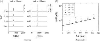
Figure 11. Streamwise velocity fluctuations at
 $Z=-5~\text{mm}$
. Case 2 (weakly unstable to secondary instability of K-type).
$Z=-5~\text{mm}$
. Case 2 (weakly unstable to secondary instability of K-type).
Large growth rates leading to larger wave amplitudes are observed in the spectra of figures 12(a) and 13(a) for cases 3 and 4, respectively. Yet at the last stations, the signal is entirely dominated by the fundamental frequency. The results still resemble the previous cases, but the maximum amplitude close to the roughness is less distinct and seems to have moved closer to the roughness. Another difference is that the evolution departs substantially from LST at the last stations, but in turn are consistent with the nonlinear behaviour predicted by the maps in figure 3(a,b).

Figure 12. Streamwise velocity fluctuations at
 $Z=-5~\text{mm}$
. Case 3 (unstable to secondary instability of K-type).
$Z=-5~\text{mm}$
. Case 3 (unstable to secondary instability of K-type).

Figure 13. Streamwise velocity fluctuations at
 $Z=-5~\text{mm}$
. Case 4 (unstable to secondary instability of K-type).
$Z=-5~\text{mm}$
. Case 4 (unstable to secondary instability of K-type).
Figure 14 displays phase distortions of TS waves for a number of flow regimes and roughness heights. Curves show distortion with respect to the case of nominally zero roughness height. In the present scenario, variations of phase are assigned either to the roughness near field or to the high amplitude of oblique waves. Distortions induced by the roughness tend to be more pronounced at early streamwise stations. At these locations, phase distortions are expected to be independent of the wave amplitude. According to the figure 14, this is indeed the case. In addition, the levels of phase distortion observed at such locations are rather small. At the other end, distortions associated with resonant wave interactions are expected to be more evident for unstable regimes and for stations far from the roughness. This is corroborated by results illustrated in figure 14. According to the figure, only unstable cases display significant phase distortion far downstream from the roughness. Stable and marginally unstable regimes show a fairly small phase distortion, at the last streamwise station. In general the phase plots also convey the idea that, flow effects that could be attributed exclusively by the roughness are restricted to the roughness vicinity and that far from the roughness the oscillations are consistent with linear or nonlinear theory as depicted in figure 3.

Figure 14. Phase distortion measured experimentally with respect to the case of nominally zero roughness height.
Detailed information about wave evolution can be extracted from the spanwise wavenumber spectra of the disturbances. For instance, the role of the secondary instability is better investigated in spectral domain. According to figures 10(a), 11(a), 12(a) and 13(a), the analysis can be restricted to the fundamental frequency. Figures 15–18 show the evolution of spanwise wavenumber spectra for a number of roughness heights. The two-dimensional component, corresponding to spanwise wavenumber (
 $\unicode[STIX]{x1D6FD}$
) equal to zero in the horizontal axis of the figure, is removed in order to enhance the observation of oblique waves. Also, the axis coordinate is displayed in
$\unicode[STIX]{x1D6FD}$
) equal to zero in the horizontal axis of the figure, is removed in order to enhance the observation of oblique waves. Also, the axis coordinate is displayed in
 $\text{mm}^{-1}$
instead of
$\text{mm}^{-1}$
instead of
 $\text{rad}~\text{mm}^{-1}$
to facilitate comparison with the roughness diameter, which is 10 mm.
$\text{rad}~\text{mm}^{-1}$
to facilitate comparison with the roughness diameter, which is 10 mm.
The spectral evolution of TS waves downstream from the roughness is shown in figures 15–18, where symbols correspond to experimental results. For all cases studied, at stations close to the roughness, amplitudes of oblique waves at fundamental frequency are approximately two orders of magnitude smaller than the two-dimensional one, because just a small portion of the incoming wave is transformed into oblique disturbances. Indeed, for cases 1 and 2, the situation holds true for nearly all streamwise stations. Under this circumstances, phase variation measured along the spanwise direction would be very small as they would mostly be associated with the excited 2-D wave, while possible contributions of the small oblique disturbances could be within the experimental uncertainty. Moreover, small phase variations of the order of few degrees caused by, for example, atmospheric wind gusts, can spread significant amount of noise into the phase of the components of the spanwise wavenumber spectra. In view of that, in the signal processing only wave magnitudes rather than the complex amplitude (with magnitudes and phases) are used in cases of oblique waves with very small amplitude. Accordingly, this procedure is adopted in producing figures 15 and 16 and the first two stations of the unstable cases 3 and 4, in figures 17 and 18. It artificially produced symmetrical spectral distributions. The procedure enhances the wave magnitude information at the expense of the phase. This simplification is applied only at situations of very small phase distortions, according to figure 14. Where, from figure 14 the phase distortion was observed to be large, the procedure was avoided.

Figure 15. Spectra of spanwise wavenumbers. ○ – experiment, – – LST calculations. Case 1.
The spectral evolution of TS waves downstream from the roughness under stable flow conditions (case1) are shown in figure 15. Dashed lines represent LST performed for a Blasius base flow. It is important to emphasize here that no base flow distortion is considered in the simulations and hence, a two-dimensional base flow condition is assumed in all simulations. For case 1, linear stability calculations are used, instead of PSE ones, in order to emphasize the weak influence of nonlinear effects. The initial amplitude distribution required to build the theoretical curve is taken from the experimental results at the first measurement station. Thus, only the evolution of disturbances generated at the roughness are analysed at this point. For small roughness heights, say up to
 $0.1\unicode[STIX]{x1D6FF}^{\ast }$
or
$0.1\unicode[STIX]{x1D6FF}^{\ast }$
or
 $0.2\unicode[STIX]{x1D6FF}^{\ast }$
the experimental and numerical comparison shows discrepancies at intermediate stations, but agrees remarkably better at the later stages. It once more conveys the idea that, for such heights, the wake influences only a region restricted to the vicinity of the roughness and that far downstream the evolution complies with that of a Blasius boundary layer excited by the spectrum at the first station. For increasingly higher roughness elements, say
$0.2\unicode[STIX]{x1D6FF}^{\ast }$
the experimental and numerical comparison shows discrepancies at intermediate stations, but agrees remarkably better at the later stages. It once more conveys the idea that, for such heights, the wake influences only a region restricted to the vicinity of the roughness and that far downstream the evolution complies with that of a Blasius boundary layer excited by the spectrum at the first station. For increasingly higher roughness elements, say
 $0.3\unicode[STIX]{x1D6FF}^{\ast }$
the roughness may have a more permanent impact. The spectra tend to broaden and for small spanwise wavenumbers, a lower amplification of disturbances in comparison to the theoretical predictions is observed. These findings are somewhat in line with works of Cossu & Brandt (Reference Cossu and Brandt2004) and Fransson et al. (Reference Fransson, Brandt, Talamelli and Cossu2005) which describe and substantiate possible damping mechanisms for 2-D TS waves interacting with high roughness elements. However, a connection with present results is purely speculative since in the works of Cossu & Brandt (Reference Cossu and Brandt2004) and Fransson et al. (Reference Fransson, Brandt, Talamelli and Cossu2005) the wave damping and the mean flow distortions are far more significant than those of present observations.
$0.3\unicode[STIX]{x1D6FF}^{\ast }$
the roughness may have a more permanent impact. The spectra tend to broaden and for small spanwise wavenumbers, a lower amplification of disturbances in comparison to the theoretical predictions is observed. These findings are somewhat in line with works of Cossu & Brandt (Reference Cossu and Brandt2004) and Fransson et al. (Reference Fransson, Brandt, Talamelli and Cossu2005) which describe and substantiate possible damping mechanisms for 2-D TS waves interacting with high roughness elements. However, a connection with present results is purely speculative since in the works of Cossu & Brandt (Reference Cossu and Brandt2004) and Fransson et al. (Reference Fransson, Brandt, Talamelli and Cossu2005) the wave damping and the mean flow distortions are far more significant than those of present observations.

Figure 16. Spectra of spanwise wavenumbers. ○ – experiment, – – nonlinear PSE calculations. Case 2.
Results obtained for marginally unstable conditions (case 2) are depicted in figure 16. Lines in the graphs correspond to weakly nonlinear calculations provided by the nonlinear PSE code. Base flow condition of two-dimensional Blasius boundary layer is also used for nonlinear PSE simulations. As in case 1, initial magnitudes used to build the theoretical spectra are taken from the experimental results at
 $\unicode[STIX]{x0394}X=25~\text{mm}$
. The spectral distributions show a double peak structure far from the roughness. The maximum amplitude is observed at wavenumbers close to
$\unicode[STIX]{x0394}X=25~\text{mm}$
. The spectral distributions show a double peak structure far from the roughness. The maximum amplitude is observed at wavenumbers close to
 $0.03~\text{mm}^{-1}$
. For roughness elements shallower than 0.1 of
$0.03~\text{mm}^{-1}$
. For roughness elements shallower than 0.1 of
 $\unicode[STIX]{x1D6FF}^{\ast }$
a fair agreement between experiments and theory is seen. Thus, secondary instability is apparently triggered by the roughness, as suggested in the works of Ustinov (Reference Ustinov1995), Crouch (Reference Crouch1997), Wang (Reference Wang2004), de Paula et al. (Reference de Paula, Medeiros and Würz2008). But for high roughness elements (
$\unicode[STIX]{x1D6FF}^{\ast }$
a fair agreement between experiments and theory is seen. Thus, secondary instability is apparently triggered by the roughness, as suggested in the works of Ustinov (Reference Ustinov1995), Crouch (Reference Crouch1997), Wang (Reference Wang2004), de Paula et al. (Reference de Paula, Medeiros and Würz2008). But for high roughness elements (
 $=0.3\unicode[STIX]{x1D6FF}^{\ast }$
) a significantly broader spectral distribution is observed in comparison with the PSE calculations. It suggests that the condition of two-dimensional base flow, adopted in the model, might be too artificial to capture the physics of the problem for such values of roughness height and this issue is further addressed in the next section.
$=0.3\unicode[STIX]{x1D6FF}^{\ast }$
) a significantly broader spectral distribution is observed in comparison with the PSE calculations. It suggests that the condition of two-dimensional base flow, adopted in the model, might be too artificial to capture the physics of the problem for such values of roughness height and this issue is further addressed in the next section.

Figure 17. Spectra of spanwise wavenumbers. ○ – experiment, – – nonlinear PSE calculations. Case 3.

Figure 18. Spectra of spanwise wavenumbers. ○ – experiment, – – nonlinear PSE calculations. Case 4.
For roughness elements shallower than 0.1 of
 $\unicode[STIX]{x1D6FF}^{\ast }$
a fair agreement between experiments and theory is seen. Thus, secondary instability is apparently triggered by the roughness, as suggested in the works of Ustinov (Reference Ustinov1995), Crouch (Reference Crouch1997), Wang (Reference Wang2004), de Paula et al. (Reference de Paula, Medeiros and Würz2008). Yet for higher roughness elements, in line with case 1, a somewhat broader spectral distribution is observed in comparison with the PSE calculations. It suggests that the condition of two-dimensional base flow, adopted in the model, might be insufficient to capture all the physics of the problem for such values of roughness height, but captures the dominant part.
$\unicode[STIX]{x1D6FF}^{\ast }$
a fair agreement between experiments and theory is seen. Thus, secondary instability is apparently triggered by the roughness, as suggested in the works of Ustinov (Reference Ustinov1995), Crouch (Reference Crouch1997), Wang (Reference Wang2004), de Paula et al. (Reference de Paula, Medeiros and Würz2008). Yet for higher roughness elements, in line with case 1, a somewhat broader spectral distribution is observed in comparison with the PSE calculations. It suggests that the condition of two-dimensional base flow, adopted in the model, might be insufficient to capture all the physics of the problem for such values of roughness height, but captures the dominant part.
Disturbances at conditions of case 3 are analysed in figure 17. Spectra show a double peak structure with a maximum amplitude located at wavenumbers close to
 $0.1~\text{mm}^{-1}$
. Again, the secondary instability is apparently triggered by the roughness,. For roughness with heights up to 0.2 of
$0.1~\text{mm}^{-1}$
. Again, the secondary instability is apparently triggered by the roughness,. For roughness with heights up to 0.2 of
 $\unicode[STIX]{x1D6FF}^{\ast }$
, the agreement between the predictions and the experiments is still fair for the dominant part of the spectra. For elements higher than
$\unicode[STIX]{x1D6FF}^{\ast }$
, the agreement between the predictions and the experiments is still fair for the dominant part of the spectra. For elements higher than
 $0.2\unicode[STIX]{x1D6FF}^{\ast }$
the predictions strongly disagreed with the experimental findings. In this last situation, the spectrum shows a four peak structure and the spanwise wavenumbers of the most amplified disturbances do not match the PSE predictions. A similar behaviour is observed for the unstable conditions of case 4, shown in figure 18, except that the modes modes predicted by the secondary instability are still dominant even for the largest roughness tested.
$0.2\unicode[STIX]{x1D6FF}^{\ast }$
the predictions strongly disagreed with the experimental findings. In this last situation, the spectrum shows a four peak structure and the spanwise wavenumbers of the most amplified disturbances do not match the PSE predictions. A similar behaviour is observed for the unstable conditions of case 4, shown in figure 18, except that the modes modes predicted by the secondary instability are still dominant even for the largest roughness tested.
Overall, results indicate that secondary instability of K-type is the most prominent nonlinear mechanism triggered by interaction between a roughness element and a plane TS wave at conditions examined in this work. It is important to mention that the nonlinear route described here is not unique and different nonlinear interactions may take place at an airfoil leading edge (Plogmann et al. Reference Plogmann, Würz and Krämer2014).
According to results of figures 15–18, it can be stated that the asymptotic evolution of disturbances in the wake of medium sized roughness elements with heights of approximately
 $0.2\unicode[STIX]{x1D6FF}^{\ast }$
, can be reasonably well predicted using a model based on an unmodified base flow. As anticipated at the beginning of this section, this conclusion fully ignores a very important aspect of the problem, which is even the key one: the mechanism of transformation of primary 2-D TS wave into 3-D TS waves due to scattering on the surface roughness. This aspect is excluded from the consideration by normalization of all spectra discussed above by the initial experimental spectrum. Therefore, the next section is devoted to the scattering of 2-D TS waves at the roughness.
$0.2\unicode[STIX]{x1D6FF}^{\ast }$
, can be reasonably well predicted using a model based on an unmodified base flow. As anticipated at the beginning of this section, this conclusion fully ignores a very important aspect of the problem, which is even the key one: the mechanism of transformation of primary 2-D TS wave into 3-D TS waves due to scattering on the surface roughness. This aspect is excluded from the consideration by normalization of all spectra discussed above by the initial experimental spectrum. Therefore, the next section is devoted to the scattering of 2-D TS waves at the roughness.
4 Scattering of TS waves at the roughness
Although models based on linear and nonlinear disturbance equations at condition of constant base flow can describe qualitatively the evolution of TS waves in the wake of a shallow roughness element, in particular far from the roughness, they are not capable to predict their amplitude just downstream of the roughness, which is what feeds the secondary instability and we here call initial amplitude. Therefore, a more detailed investigation is necessary to find how initial amplitudes of 3-D waves scale with roughness height, shape and TS amplitude. In principle, local variations of the base flow induced by the roughness might be an important source of three-dimensionality. Thus, the role of this mechanism on the initial amplitude of 3-D TS waves is assessed in the following section. In addition, linear interactions between the roughness and the TS waves are analysed. This last case configures a linear transfer function problem. The term scattering function is used here to designate the linear transfer function for scattering of 2-D waves at the roughness. Although in the scattering problem a different source is responsible for the excitation of oblique waves than in receptivity problems, the linear transfer functions of both phenomena are rather similar. Thus, the methodology applied here to address this topic is based on receptivity studies of Saric et al. (Reference Saric, Hoos, Radeztsky, Reda, Reed and Kobayashi1991), Choudhari & Streett (Reference Choudhari and Streett1992), Crouch (Reference Crouch1994), Kachanov (Reference Kachanov2000) and Würz et al. (Reference Würz, Herr, Wörner, Rist, Wagner and Kachanov2003).
4.1 Initial spectra of disturbances in the roughness wake
Prior to estimating the scattering function, measured disturbances are analysed in detail at the first measurement station. Initially the scaling of the 3-D disturbance amplitudes with respect to the amplitude of the 2-D TS wave at the roughness location (
 $A_{0}$
) is investigated. The spectra of spanwise wavenumbers displayed in the figure 19(a,b) are normalized by
$A_{0}$
) is investigated. The spectra of spanwise wavenumbers displayed in the figure 19(a,b) are normalized by
 $A_{0}$
. Results shown in figure 19(a) correspond to cases 1 and 3, while figure 19(b) is for cases 2 and 4. For the sake of clarity, the 2-D mode, corresponding to
$A_{0}$
. Results shown in figure 19(a) correspond to cases 1 and 3, while figure 19(b) is for cases 2 and 4. For the sake of clarity, the 2-D mode, corresponding to
 $\unicode[STIX]{x1D6FD}$
equals to 0 is not shown. Within the experimental range, for a given TS frequency, the initial amplitude of the 3-D disturbances scale linearly with the 2-D wave amplitude.
$\unicode[STIX]{x1D6FD}$
equals to 0 is not shown. Within the experimental range, for a given TS frequency, the initial amplitude of the 3-D disturbances scale linearly with the 2-D wave amplitude.

Figure 19. Spectra of disturbances at
 $\unicode[STIX]{x0394}X=25~\text{mm}$
normalized by TS wave amplitude at the roughness (
$\unicode[STIX]{x0394}X=25~\text{mm}$
normalized by TS wave amplitude at the roughness (
 $A_{0}$
). Open symbols:
$A_{0}$
). Open symbols:
 $A_{0}=0.45\,\%$
; filled symbols:
$A_{0}=0.45\,\%$
; filled symbols:
 $A_{0}=0.75\,\%$
. (a) Cases 1 and 3; (b) Cases 2 and 4.
$A_{0}=0.75\,\%$
. (a) Cases 1 and 3; (b) Cases 2 and 4.
According to figure 19(a,b), the roughness height can influence the initial spectra of disturbances. The side lobes of the curves are shifted toward higher wavenumbers as the roughness height increases. For instance, in figure 19(a,b) the peak in the first side lobe of the spectra is shifted from 0.1 to
 $0.16~\text{mm}^{-1}$
as the roughness height is increased from 0.1 to
$0.16~\text{mm}^{-1}$
as the roughness height is increased from 0.1 to
 $0.3h/\unicode[STIX]{x1D6FF}^{\ast }$
, respectively. Since the roughness shape is not changed, the flow reaction responsible for generation of 3-D disturbances is what must have varied with the roughness height. For high roughness elements, measurements displayed in figures 15, 16, 17, 18 indicate a modification in the evolution of TS waves at the roughness wake. In figure 19(a,b), results show modifications also in the initial amplitude of disturbances.
$0.3h/\unicode[STIX]{x1D6FF}^{\ast }$
, respectively. Since the roughness shape is not changed, the flow reaction responsible for generation of 3-D disturbances is what must have varied with the roughness height. For high roughness elements, measurements displayed in figures 15, 16, 17, 18 indicate a modification in the evolution of TS waves at the roughness wake. In figure 19(a,b), results show modifications also in the initial amplitude of disturbances.
In order to shed more light onto the mechanisms involved in the scattering of disturbances by the roughness, the mean flow distortion (MFD) is analysed for different roughness heights. Curves given in figure 20 cover all regimes investigated. The distortion at the first station is estimated by subtracting the reference case from the measured data. The reference corresponds to the roughness retracted (
 $h\approx 0$
) case. The solid line gives the spectrum of the roughness cross-section.
$h\approx 0$
) case. The solid line gives the spectrum of the roughness cross-section.

Figure 20. Symbols: mean flow distortion at
 $\unicode[STIX]{x0394}X=25~\text{mm}$
for different roughness heights. Line: Fourier transform of the roughness cross-section. It corresponds to the component of the roughness spectra at zero streamwise wavenumber
$\unicode[STIX]{x0394}X=25~\text{mm}$
for different roughness heights. Line: Fourier transform of the roughness cross-section. It corresponds to the component of the roughness spectra at zero streamwise wavenumber
 $\unicode[STIX]{x1D6FC}=0$
.
$\unicode[STIX]{x1D6FC}=0$
.
According to figure 20(a) weak MFDs are present when
 $h$
is close to
$h$
is close to
 $0.1\unicode[STIX]{x1D6FF}^{\ast }$
. Moreover, no agreement is found between the roughness shape spectrum and the spectrum of the base flow distortions. In this case, the amplitude of mean flow distortions associated with the roughness element appears to be within the experimental noise.
$0.1\unicode[STIX]{x1D6FF}^{\ast }$
. Moreover, no agreement is found between the roughness shape spectrum and the spectrum of the base flow distortions. In this case, the amplitude of mean flow distortions associated with the roughness element appears to be within the experimental noise.
In the case of high roughness elements (
 $0.3\unicode[STIX]{x1D6FF}^{\ast }$
) the spectral distribution of MFD is remarkably different and close to the roughness spectra, as shown figure 20(c). Moreover, the spectral distribution is not strongly dependent on TS frequency or amplitude. Therefore, the MFD in this case seems to be determined by the roughness. Results for intermediate roughness height
$0.3\unicode[STIX]{x1D6FF}^{\ast }$
) the spectral distribution of MFD is remarkably different and close to the roughness spectra, as shown figure 20(c). Moreover, the spectral distribution is not strongly dependent on TS frequency or amplitude. Therefore, the MFD in this case seems to be determined by the roughness. Results for intermediate roughness height
 $0.2\unicode[STIX]{x1D6FF}^{\ast }$
indicate a gradual variation from one limiting case to the other (see figure 20
c). Overall the picture shows that substantial mean flow distortions are present only for relatively high roughness. For low roughness a wave scattering is the most promising disturbance mechanism induced by the roughness. Also interesting is that, for all cases considered, the experimental curves do not display strong influence of the TS wave amplitude or frequency on the mean flow distortion.
$0.2\unicode[STIX]{x1D6FF}^{\ast }$
indicate a gradual variation from one limiting case to the other (see figure 20
c). Overall the picture shows that substantial mean flow distortions are present only for relatively high roughness. For low roughness a wave scattering is the most promising disturbance mechanism induced by the roughness. Also interesting is that, for all cases considered, the experimental curves do not display strong influence of the TS wave amplitude or frequency on the mean flow distortion.
A comparative analysis of TS wave amplitudes and mean flow distortions at the first station is provided in figure 21. Curves are normalized by their maximum to facilitate a direct comparison between the spectra. According to figures 19 and 20, results obtained at the first station for cases 1 and 2 are very similar to those observed for cases 3 ad 4, respectively. Therefore, for clarity only results of cases 1 and 2 are displayed in figure 21. Nevertheless, conclusions and comments drawn for these cases can be extended also to cases 3 and 4. In figure 21(a,b) no clear connection between the TS waves and the mean flow distortion is seen for shallow and moderate roughness heights. For these cases, the wave scattering into three-dimensional disturbances is weakly dependent of the MFD. Results obtained for high roughness elements, shown in figure 21(c), suggest a close link between the TS waves and the MFD. Therefore, in the scenario investigated here the mean flow distortion induced by relatively high roughness elements (
 $h/\unicode[STIX]{x1D6FF}^{\ast }>0.2$
) can strongly influence the initial amplitudes of 3-D disturbances.
$h/\unicode[STIX]{x1D6FF}^{\ast }>0.2$
) can strongly influence the initial amplitudes of 3-D disturbances.
The influence of MFD on the initial spectra of disturbances certainly reduce the accuracy of models based only on wave scattering. The next section is devoted to performing an analysis of the scattering problem including an assessment of the model for moderate roughness heights.

Figure 21. Comparison of normalized spectra of disturbances and mean flow distortion at
 $\unicode[STIX]{x0394}X=25~\text{mm}$
.
$\unicode[STIX]{x0394}X=25~\text{mm}$
.
4.2 Transfer function for TS wave scattering at shallow roughness
In the following analysis, the roughness shape is represented in terms of spanwise and streamwise wavenumbers, according to Crouch (Reference Crouch1994), Kachanov (Reference Kachanov2000) and Würz et al. (Reference Würz, Herr, Wörner, Rist, Wagner and Kachanov2003). The spectrum shown in figure 22 is obtained by applying a two-dimensional Fourier transform to the roughness shape. The figure also includes the dispersion curves of
 $\unicode[STIX]{x1D6FC}$
as a function of
$\unicode[STIX]{x1D6FC}$
as a function of
 $\unicode[STIX]{x1D6FD}$
for fixed frequencies of a TS wave and Reynolds number. Dispersion curves shown in the figure are associated with the frequencies tested in the experiment. Magnitudes and phases of the 2-D roughness spectrum, for unit roughness height, at streamwise and spanwise wavenumbers given by the dispersion curve, correspond to the resonant spectrum (
$\unicode[STIX]{x1D6FD}$
for fixed frequencies of a TS wave and Reynolds number. Dispersion curves shown in the figure are associated with the frequencies tested in the experiment. Magnitudes and phases of the 2-D roughness spectrum, for unit roughness height, at streamwise and spanwise wavenumbers given by the dispersion curve, correspond to the resonant spectrum (
 $H(\unicode[STIX]{x1D6FC},\unicode[STIX]{x1D6FD})$
). Thereby, it is possible to use the following equation for estimating the linear scattering function
$H(\unicode[STIX]{x1D6FC},\unicode[STIX]{x1D6FD})$
). Thereby, it is possible to use the following equation for estimating the linear scattering function
 $G$
:
$G$
:
 $$\begin{eqnarray}G(\unicode[STIX]{x1D6FC},\unicode[STIX]{x1D6FD})=\frac{[A(\unicode[STIX]{x1D6FC},\unicode[STIX]{x1D6FD},h\neq 0,\unicode[STIX]{x0394}X=0)-A(\unicode[STIX]{x1D6FC},\unicode[STIX]{x1D6FD},h=0,\unicode[STIX]{x0394}X=0)]}{H_{norm}(\unicode[STIX]{x1D6FC},\unicode[STIX]{x1D6FD})\,A_{0}\,h/\unicode[STIX]{x1D6FF}^{\ast }}.\end{eqnarray}$$
Although the equation shows no restriction with respect to
 $\unicode[STIX]{x1D6FD}$
, only cases related to 3-D waves (
$\unicode[STIX]{x1D6FD}$
, only cases related to 3-D waves (
 $\unicode[STIX]{x1D6FD}\neq 0$
) are analysed here.
$\unicode[STIX]{x1D6FD}\neq 0$
) are analysed here.
Equation(4.1) is very similar to acoustic receptivity functions from the works of Kachanov (Reference Kachanov2000) and Würz et al. (Reference Würz, Herr, Wörner, Rist, Wagner and Kachanov2003). Here, the main difference with respect to the literature is, firstly, the normalization of the resonant spectrum calculated for unit roughness height (
 $H$
) which is divided by its maximum amplitude (
$H$
) which is divided by its maximum amplitude (
 $H_{norm}=H/\max (H)$
), and secondly, the forcing disturbance which is the TS wave. The normalization is performed for each wave frequency, because amplitudes of
$H_{norm}=H/\max (H)$
), and secondly, the forcing disturbance which is the TS wave. The normalization is performed for each wave frequency, because amplitudes of
 $H$
, in the roughness spectra of figure 22, can vary significantly for different TS wave frequencies. However, figure 19(a,b) shows similar amplitude levels of scattered waves measured for two excitation frequencies. Thus, the normalized resonant spectrum was assumed to represent better the experimental results.
$H$
, in the roughness spectra of figure 22, can vary significantly for different TS wave frequencies. However, figure 19(a,b) shows similar amplitude levels of scattered waves measured for two excitation frequencies. Thus, the normalized resonant spectrum was assumed to represent better the experimental results.

Figure 22. Spectral distribution for a unit height roughness element and dispersion curves of TS waves (lines).
As explained in § 3, of the current work, at the earlier measurement stations, only magnitudes are considered, hence the phase of the receptivity function is not determined. As a consequence, phases of oblique waves in (4.1) are assumed to be all equal to the phase of the incoming plane wave. This assumption is supported by results of figure 14.
In the following, the roughness resonant spectra are compared against experimental data at the first measurement station. To this end, the theoretical growth rates provided by LST are used to extrapolate amplitudes of the roughness resonant spectra (
 $\unicode[STIX]{x0394}X=0$
) to the first measurement station (
$\unicode[STIX]{x0394}X=0$
) to the first measurement station (
 $\unicode[STIX]{x0394}X=25~\text{mm}$
). The experimental results are subtracted by the reference case of nominally zero roughness height before being shown in figure 23. Thereby, the influence of the excited TS wave is removed and only disturbances introduced by the interaction with the roughness are considered. For small roughness elements results of figure 23 show a fair agreement with the model. There is an evident amplitude difference in the side lobes of the curves, which points to a higher efficiency in excitation of oblique waves in comparison with two-dimensional ones. Many works, such as Choudhari & Streett (Reference Choudhari and Streett1992), Crouch (Reference Crouch1994), Kachanov (Reference Kachanov2000) and Würz et al. (Reference Würz, Herr, Wörner, Rist, Wagner and Kachanov2003), report a similar behaviour for acoustic receptivity induced by roughness. The experimental spectra distribution shown in figure 23, are similar for roughness within a range from 0.05 to
$\unicode[STIX]{x0394}X=25~\text{mm}$
). The experimental results are subtracted by the reference case of nominally zero roughness height before being shown in figure 23. Thereby, the influence of the excited TS wave is removed and only disturbances introduced by the interaction with the roughness are considered. For small roughness elements results of figure 23 show a fair agreement with the model. There is an evident amplitude difference in the side lobes of the curves, which points to a higher efficiency in excitation of oblique waves in comparison with two-dimensional ones. Many works, such as Choudhari & Streett (Reference Choudhari and Streett1992), Crouch (Reference Crouch1994), Kachanov (Reference Kachanov2000) and Würz et al. (Reference Würz, Herr, Wörner, Rist, Wagner and Kachanov2003), report a similar behaviour for acoustic receptivity induced by roughness. The experimental spectra distribution shown in figure 23, are similar for roughness within a range from 0.05 to
 $0.15h/\unicode[STIX]{x1D6FF}^{\ast }$
. For roughness elements around
$0.15h/\unicode[STIX]{x1D6FF}^{\ast }$
. For roughness elements around
 $0.2\unicode[STIX]{x1D6FF}^{\ast }$
the spectral distribution became slightly different. Above this height the distribution is very different and the transfer of energy from 2-D to 3-D waves seems to be strongly affected by the MFD (see figure 21). Thus, it is not appropriate to use linear scattering approach for modelling the roughness effect under these circumstances. Therefore, the following analysis focuses on roughness elements up to
$0.2\unicode[STIX]{x1D6FF}^{\ast }$
the spectral distribution became slightly different. Above this height the distribution is very different and the transfer of energy from 2-D to 3-D waves seems to be strongly affected by the MFD (see figure 21). Thus, it is not appropriate to use linear scattering approach for modelling the roughness effect under these circumstances. Therefore, the following analysis focuses on roughness elements up to
 $0.2\unicode[STIX]{x1D6FF}^{\ast }$
.
$0.2\unicode[STIX]{x1D6FF}^{\ast }$
.

Figure 23. Comparison of wave distribution observed at
 $\unicode[STIX]{x0394}X=25~\text{mm}$
with respective roughness spectrum. For a proper comparison, amplitudes of the roughness spectrum are multiplied by the corresponding amplification from
$\unicode[STIX]{x0394}X=25~\text{mm}$
with respective roughness spectrum. For a proper comparison, amplitudes of the roughness spectrum are multiplied by the corresponding amplification from
 $\unicode[STIX]{x0394}X=0$
to 25 mm according to LST. (a) Case 1, (b) case (2).
$\unicode[STIX]{x0394}X=0$
to 25 mm according to LST. (a) Case 1, (b) case (2).
In principle, the linear scattering function can be easily calculated using (4.1). However, amplitudes cannot be directly applied into the equation due to zeros in the roughness spectra of figure 23. In order to avoid division by zero, calculations are performed using the amplitude envelope of the spectral distribution. To compute the envelope amplitude, a Hilbert transform is applied to the experimental data and to the roughness resonant spectra, as illustrated in figure 24. For clarity, each curve is normalized by its absolute maximum amplitude. The experimental envelope is calculated for the case with a roughness height equals to a
 $0.05\unicode[STIX]{x1D6FF}\ast$
. According to results of figure 23 for this height there is no influence of the mean flow distortion on the results. In any case, results close to the zeros of the roughness spectra are likely to be less accurate.
$0.05\unicode[STIX]{x1D6FF}\ast$
. According to results of figure 23 for this height there is no influence of the mean flow distortion on the results. In any case, results close to the zeros of the roughness spectra are likely to be less accurate.

Figure 24. Envelope amplitude of the spectral distribution of the roughness-induced disturbances at
 $\unicode[STIX]{x0394}X=25~\text{mm}$
. For a proper comparison, amplitudes of the roughness spectrum are multiplied by the corresponding amplification from
$\unicode[STIX]{x0394}X=25~\text{mm}$
. For a proper comparison, amplitudes of the roughness spectrum are multiplied by the corresponding amplification from
 $\unicode[STIX]{x0394}X=0$
to 25 mm according to LST. (a) Case 1, (b) case 2.
$\unicode[STIX]{x0394}X=0$
to 25 mm according to LST. (a) Case 1, (b) case 2.
Finally, magnitudes of the scattering function are estimated according to (4.1). It is convenient to present the scattering function by means of the wave angle,
 $\unicode[STIX]{x1D703}=\tan ^{-1}(\unicode[STIX]{x1D6FD}/\unicode[STIX]{x1D6FC})$
, for each given TS wave frequency to facilitate comparison with the literature. Results are presented for propagation angles between
$\unicode[STIX]{x1D703}=\tan ^{-1}(\unicode[STIX]{x1D6FD}/\unicode[STIX]{x1D6FC})$
, for each given TS wave frequency to facilitate comparison with the literature. Results are presented for propagation angles between
 $\pm 45^{\circ }$
. In terms of spanwise wavenumbers this range corresponds, approximately, to
$\pm 45^{\circ }$
. In terms of spanwise wavenumbers this range corresponds, approximately, to
 $\pm 0.2~\text{mm}^{-1}$
.
$\pm 0.2~\text{mm}^{-1}$
.
In figure 25, open symbols are related to cases 1 and 2. They display a similar variation within the range of frequencies and dispersion angles analysed. Results suggest a weak sensitivity of the functions with respect to the wave frequency. Moreover, the graphics quantify the anticipated result of higher scattering coefficients for oblique waves in comparison to two-dimensional ones. For illustration, the current findings are compared with acoustic receptivity results from Würz et al. (Reference Würz, Herr, Wörner, Rist, Wagner and Kachanov2003). The similarity between scattering and receptivity functions is remarkable in view that the mechanisms are rather different.

Figure 25. Estimated scattering coefficients. Comparison with acoustic receptivity coefficients found in the work of Würz et al. (Reference Würz, Herr, Wörner, Rist, Wagner and Kachanov2003).
4.3 Extension of the scattering function to higher roughness elements
Linear scattering functions of the type discussed in this work can be used to predict initial amplitudes of oblique waves for any particular roughness geometry, incoming wave amplitude and frequency. In the usual methodology, the roughness height is assumed to influence linearly the amplitude of the excited disturbances. However, the range where this assumption is valid is not known a priori. In order to explore the influence of the roughness height on the receptivity functions, some integrals are evaluated in a range of spanwise wavenumbers of
 $\pm 0.2~\text{mm}^{-1}$
:
$\pm 0.2~\text{mm}^{-1}$
:
 $$\begin{eqnarray}\displaystyle & \displaystyle I_{A}(\unicode[STIX]{x1D6FC},\unicode[STIX]{x1D6FD},h)=\frac{1}{2B}\int _{-B}^{+B}[A(\unicode[STIX]{x1D6FC},\unicode[STIX]{x1D6FD},h,\unicode[STIX]{x0394}X=0)-A(\unicode[STIX]{x1D6FC},\unicode[STIX]{x1D6FD},h=0,\unicode[STIX]{x0394}X=0)]\,\unicode[STIX]{x2202}\unicode[STIX]{x1D6FD}, & \displaystyle\end{eqnarray}$$
 $$\begin{eqnarray}\displaystyle & \displaystyle I_{GHA_{0}}(\unicode[STIX]{x1D6FC},\unicode[STIX]{x1D6FD})=\frac{1}{2B}\int _{-B}^{+B}G(\unicode[STIX]{x1D6FC},\unicode[STIX]{x1D6FD})\,H_{norm}(\unicode[STIX]{x1D6FC},\unicode[STIX]{x1D6FD})\,A_{0}\,\unicode[STIX]{x2202}\unicode[STIX]{x1D6FD}. & \displaystyle\end{eqnarray}$$
The term
 $I_{A}$
in (4.2), represents an integral of the experimental spectra, while the term
$I_{A}$
in (4.2), represents an integral of the experimental spectra, while the term
 $I_{GHA_{0}}$
is related to an integral of the model predictions divided by the roughness height. In the range of validity of the linear model, the ratio given by
$I_{GHA_{0}}$
is related to an integral of the model predictions divided by the roughness height. In the range of validity of the linear model, the ratio given by
 $I_{A}/I_{GHA_{0}}$
(see figure 26) should match the non-dimensional roughness height, because this is the only parameter missing in
$I_{A}/I_{GHA_{0}}$
(see figure 26) should match the non-dimensional roughness height, because this is the only parameter missing in
 $I_{GHA_{0}}$
. However, in figure 26 the dashed line only approaches the ratio of integrals for
$I_{GHA_{0}}$
. However, in figure 26 the dashed line only approaches the ratio of integrals for
 $h/\unicode[STIX]{x1D6FF}^{\ast }$
below 0.1. For the entire range of heights investigated, the ratio is better fitted to a parabola. In addition, the ratio is not significantly changed for the two frequencies and two amplitudes analysed. Therefore, the same trend line represents cases 1 to 4.
$h/\unicode[STIX]{x1D6FF}^{\ast }$
below 0.1. For the entire range of heights investigated, the ratio is better fitted to a parabola. In addition, the ratio is not significantly changed for the two frequencies and two amplitudes analysed. Therefore, the same trend line represents cases 1 to 4.

Figure 26. Variation of integrated spectral distributions with respect to the roughness height at
 $\unicode[STIX]{x0394}X=0$
.
$\unicode[STIX]{x0394}X=0$
.
Results presented in figures 19(a,b), 23(a,b), suggest that weakly nonlinear corrections can be applied to the scattering function in order to extend its range of application. This conjecture is supported by the spectra of figure 23(a,b), which are qualitatively similar for roughness shorter than
 $0.2\unicode[STIX]{x1D6FF}^{\ast }$
. Within this range, results suggest that nonlinearities in the scattering function are related to the roughness height rather than to its shape. Thus the first nonlinear corrections for scattering coefficients in (4.1) seem to be linked to the term
$0.2\unicode[STIX]{x1D6FF}^{\ast }$
. Within this range, results suggest that nonlinearities in the scattering function are related to the roughness height rather than to its shape. Thus the first nonlinear corrections for scattering coefficients in (4.1) seem to be linked to the term
 $h/\unicode[STIX]{x1D6FF}^{\ast }$
with the term
$h/\unicode[STIX]{x1D6FF}^{\ast }$
with the term
 $H(\unicode[STIX]{x1D6FC},\unicode[STIX]{x1D6FD})$
playing a lesser role.
$H(\unicode[STIX]{x1D6FC},\unicode[STIX]{x1D6FD})$
playing a lesser role.
Here a correction due to
 $h/\unicode[STIX]{x1D6FF}^{\ast }$
is estimated from the ratio between
$h/\unicode[STIX]{x1D6FF}^{\ast }$
is estimated from the ratio between
 $I_{A}$
and
$I_{A}$
and
 $I_{GHA_{0}}$
, and is used by replacing the term
$I_{GHA_{0}}$
, and is used by replacing the term
 $h/\unicode[STIX]{x1D6FF}^{\ast }$
in (4.1) by the second-order equation given with figure 26. The equation is merely a quadratic fit to the results based on the roughness height.
$h/\unicode[STIX]{x1D6FF}^{\ast }$
in (4.1) by the second-order equation given with figure 26. The equation is merely a quadratic fit to the results based on the roughness height.
In order to evaluate the proposed correction, spectra of disturbances are estimated at the first measurement station (
 $\unicode[STIX]{x0394}X=25~\text{mm}$
) using the scattering functions and calculations based on LST. Predictions given by the model are then used as initial amplitude for oblique waves and their evolution is estimated acceding to LST and PSE calculations. For a proper comparison against experimental results, the reference spectrum related to the case of nominally zero roughness height is added to the model predictions. Thus, background disturbances that have been removed for calculations in (4.1), are added again to compose the spectra of disturbances. This is necessary because the model can only predict disturbances related to the interaction between a plane TS wave and a single roughness element. The evolution of the disturbances downstream from the first measurement station is estimated using LST, for case 1, and nonlinear PSE for cases 2, 3 and 4. For both stability calculations, the base flow condition is a non-disturbed 2-D Blasius boundary layer. The procedure is the same adopted for figures 15–18.
$\unicode[STIX]{x0394}X=25~\text{mm}$
) using the scattering functions and calculations based on LST. Predictions given by the model are then used as initial amplitude for oblique waves and their evolution is estimated acceding to LST and PSE calculations. For a proper comparison against experimental results, the reference spectrum related to the case of nominally zero roughness height is added to the model predictions. Thus, background disturbances that have been removed for calculations in (4.1), are added again to compose the spectra of disturbances. This is necessary because the model can only predict disturbances related to the interaction between a plane TS wave and a single roughness element. The evolution of the disturbances downstream from the first measurement station is estimated using LST, for case 1, and nonlinear PSE for cases 2, 3 and 4. For both stability calculations, the base flow condition is a non-disturbed 2-D Blasius boundary layer. The procedure is the same adopted for figures 15–18.

Figure 27. Evolution of the spanwise wavenumbers spectra for case 1. (○) – experiments, (– –) LST
 $+$
receptivity.
$+$
receptivity.

Figure 28. Evolution of the spanwise wavenumbers spectra for case 2. (○) – experiments, (– —) nonlinear PSE
 $+$
receptivity.
$+$
receptivity.

Figure 29. Evolution of the spanwise wavenumbers spectra for case 3. (○) – experiments, (– –) nonlinear PSE
 $+$
receptivity.
$+$
receptivity.

Figure 30. Evolution of the spanwise wavenumbers spectra for case 4. (○) – experiments, (– –) nonlinear PSE
 $+$
receptivity.
$+$
receptivity.
The scattering model with nonlinear correction based on roughness height is concerned only with the results of the first station (
 $\unicode[STIX]{x0394}X=25~\text{mm}$
) shown in figures 27–30. In general the agreement between model and experiments is good at this stations, providing strong evidence of applicability of the correction. Figures 27–30 also give the subsequent evolution of predicted waves in a fashion similar to that of figures 15–18 of the previous section. Here the agreement is not as good as in the previous section, but this is consistent with the extra level of modelling involved. It nevertheless shows the same trends, namely, better agreement far from the roughness and for smaller roughness. At some places the agreement is poor, such as for large roughness in case 4, figure 30, where the nonlinear modes are severely underpredicted. However, the disagreement can be traced to the region close to zeros of the roughness spectra, which, unfortunately, for this case fall very close to the most unstable modes of the secondary instability. Deviations at the initial condition are strongly amplified under these circumstances.
$\unicode[STIX]{x0394}X=25~\text{mm}$
) shown in figures 27–30. In general the agreement between model and experiments is good at this stations, providing strong evidence of applicability of the correction. Figures 27–30 also give the subsequent evolution of predicted waves in a fashion similar to that of figures 15–18 of the previous section. Here the agreement is not as good as in the previous section, but this is consistent with the extra level of modelling involved. It nevertheless shows the same trends, namely, better agreement far from the roughness and for smaller roughness. At some places the agreement is poor, such as for large roughness in case 4, figure 30, where the nonlinear modes are severely underpredicted. However, the disagreement can be traced to the region close to zeros of the roughness spectra, which, unfortunately, for this case fall very close to the most unstable modes of the secondary instability. Deviations at the initial condition are strongly amplified under these circumstances.
5 Conclusions
The paper reports on an experimental investigation of the interaction of a two-dimensional TS wave and an isolated roughness. The roughness was cylindrical, with a diameter of 10 mm (close to a TS wave wavelength), had sharp edges and a controlled height that could be varied within a small and medium height range (up to
 $0.3\unicode[STIX]{x1D6FF}^{\ast }$
). The roughness was positioned far from the leading edge of the model at a location of weak variation of the boundary layer thickness with the streamwise direction. The experimental work was assisted by PSE both in its planning and in the analysis of the results. Two TS wave amplitudes and two frequencies were chosen for the tests. PSE computations indicated that the TS waves used ranged from stable to unstable with respect the boundary layer secondary instability of the fundamental type.
$0.3\unicode[STIX]{x1D6FF}^{\ast }$
). The roughness was positioned far from the leading edge of the model at a location of weak variation of the boundary layer thickness with the streamwise direction. The experimental work was assisted by PSE both in its planning and in the analysis of the results. Two TS wave amplitudes and two frequencies were chosen for the tests. PSE computations indicated that the TS waves used ranged from stable to unstable with respect the boundary layer secondary instability of the fundamental type.
The work confirmed experimentally that the roughness can trigger the boundary layer secondary instability of the fundamental type. This result had been suggested by previous theoretical work, and is now generally accepted as the scenario observed by Klebanoff, Tidstrom & Sargent (Reference Klebanoff, Tidstrom and Sargent1962). For all the experiments reported, the roughness was in the subcritical regime with respect to engineering criteria for transition induced by roughness elements in a quiet boundary layer. For the scenario here studied the critical condition for transition anticipation is the TS wave amplitude and, for the parameter space covered the critical amplitude was the threshold amplitude for the secondary instability of fundamental type.
Comparison of the experimental results with PSE predictions of wave evolution in a Blasius boundary layer were also carried out. For these PSE computations the inlet condition was the spectra measured at the first measurement station downstream of the roughness. As expected, high roughness elements affected significantly the wave evolution. However, for roughness up to
 $0.2\unicode[STIX]{x1D6FF}^{\ast }$
the dominant features of the phenomenon could be predicted using a Blasius boundary layer. Very interesting was that, within this roughness height regime, deviations from the theory were more pronounced at the roughness vicinity, while the downstream asymptotic behaviour followed the theory more closely. The disagreement at intermediate stations might be related with transient growth mechanisms in the near field of high roughness elements, like those observed in Reshotko & Tumin (Reference Reshotko and Tumin2004) and Denissen & White (Reference Denissen and White2013) for yet higher roughness elements. However, this conjecture still lacks verification.
$0.2\unicode[STIX]{x1D6FF}^{\ast }$
the dominant features of the phenomenon could be predicted using a Blasius boundary layer. Very interesting was that, within this roughness height regime, deviations from the theory were more pronounced at the roughness vicinity, while the downstream asymptotic behaviour followed the theory more closely. The disagreement at intermediate stations might be related with transient growth mechanisms in the near field of high roughness elements, like those observed in Reshotko & Tumin (Reference Reshotko and Tumin2004) and Denissen & White (Reference Denissen and White2013) for yet higher roughness elements. However, this conjecture still lacks verification.
The paper also analysed and quantified the scattering of the two dimensional TS waves into three-dimensional TS waves promoted by the roughness. A methodology is proposed for estimation of scattering coefficients using envelope amplitudes of the roughness shape spectrum. Thereby, singularities introduced in the linear scattering transfer functions (see (4.1)) by zero values of the roughness spectrum are avoided. According to the suggested procedure, the magnitude of the wave scattering functions can be obtained for any arbitrary roughness shape. Within the parameter range covered in the experiments, the scattering was linear with respect to the TS wave amplitude. In addition, the scattering transfer function was found to favour oblique waves showing a remarkable similarity with acoustic receptivity functions reported in the literature (Würz et al. Reference Würz, Herr, Wörner, Rist, Wagner and Kachanov2003). Here, the shape of the scattering transfer function did not vary significantly with the TS wave frequencies tested, but the magnitude of the scattering was sensitive to this frequency.
The scattering was linear with respect to the roughness height only for very small roughness, up to approximately
 $0.08\unicode[STIX]{x1D6FF}^{\ast }$
. For slightly larger height values, the scattering was nonlinear with respect to the roughness height, but the shape of the scattering function was still not modified. This was observed for heights up to
$0.08\unicode[STIX]{x1D6FF}^{\ast }$
. For slightly larger height values, the scattering was nonlinear with respect to the roughness height, but the shape of the scattering function was still not modified. This was observed for heights up to
 $0.2\unicode[STIX]{x1D6FF}^{\ast }$
. It must be said, however, that such nonlinear behaviour was observed only for the roughness tested and it may not hold for other roughness shapes. Within this range a quadratic correction for scattering magnitude based on roughness could be fit to the data. Comparison between the scattering function model and the experimental results at the first measurement station downstream of the roughness was good for roughness up to
$0.2\unicode[STIX]{x1D6FF}^{\ast }$
. It must be said, however, that such nonlinear behaviour was observed only for the roughness tested and it may not hold for other roughness shapes. Within this range a quadratic correction for scattering magnitude based on roughness could be fit to the data. Comparison between the scattering function model and the experimental results at the first measurement station downstream of the roughness was good for roughness up to
 $0.2\unicode[STIX]{x1D6FF}^{\ast }$
.
$0.2\unicode[STIX]{x1D6FF}^{\ast }$
.
Comparison of the experimental evolution of the wave system and that computed by PSE considering a Blasius profile was once more performed. This time the inlet conditions for the PSE was the result of the nonlinearly corrected scattering function. Obviously the agreement was not as good as in cases with PSE computations initiated with experimental results, since it has an extra step of modelling. It however was consistent with previous computations revealing similar trends. Overall, the work quantified, for this roughness, to which extent the dominant feature in this scenario is simply the scattering of the TS waves at the roughness.
From a practical perspective, results suggest that models developed for transition prediction in smooth surfaces can be somehow extended to include roughness elements with heights up to
 $0.2\unicode[STIX]{x1D6FF}^{\ast }$
. It is expected that the current findings could guide future works towards a parametric examination of the aspects raised by this investigation. This might support the development of new transition prediction tools that account for the influence of medium sized roughness.
$0.2\unicode[STIX]{x1D6FF}^{\ast }$
. It is expected that the current findings could guide future works towards a parametric examination of the aspects raised by this investigation. This might support the development of new transition prediction tools that account for the influence of medium sized roughness.
Acknowledgements
This work was supported by the CAPES
 $BEX2443/04-0$
and FAPESP
$BEX2443/04-0$
and FAPESP
 $02/05818-7$
, both from Brazil. M.A.F.M. thanks the National Council for Scientific and Technological Development CNPq/Brazil for support via project 304243/2013-2.
$02/05818-7$
, both from Brazil. M.A.F.M. thanks the National Council for Scientific and Technological Development CNPq/Brazil for support via project 304243/2013-2.


