


Introduction
The Cassini Mission discovered jets of fine icy particles lofted by water vapour and venting from rifts in the ice cover of Enceladus (Hansen et al. Reference Hansen, Esposito, Stewart, Colwell, Hendrix, Pryor, Shemansky and West2006; Porco et al. Reference Porco, Helfenstein, Thomas, Ingersoll, Wisdom, West, Neukum, Denk, Wagner, Roatsch, Kieffer, Turtle, McEwen, Johnson, Rathbun, Veverka, Wilson, Perry, Spitale, Brahic, Burns, Delgenio, Dones, Murray and Squyres2006; Spencer et al. Reference Spencer, Pearl, Segura, Flasar, Mamoutkine, Romani, Buratti, Hendrix, Spilker and Lopes2006; Waite et al. Reference Waite, Combi, Ip, Cravens, McNutt, Kasprzak, Yelle, Luhmann, Niemann, Gell, Magee, Fletcher, Lunine and Tseng2006). This plume has been investigated extensively as the Cassini spacecraft passed through the plume multiple times over the course of a decade at elevations ranging from 50 to hundreds of kilometers and at relative velocities from ~6 to 18 km s−1. The data from these flybys indicate that the plume originates from a global ocean below an ice crust approximately 10–40 km thick (Iess et al. Reference Iess, Stevenson, Parisi, Hemingway, Jacobson, Lunine, Nimmo, Armstrong, Asmar, Ducci and Tortora2014; Thomas et al. Reference Thomas, Tajeddine, Tiscareno, Burns, Joseph, Loredo, Helfenstein and Porco2016) and maybe even <5 km thick at the south pole region (Čadek et al. Reference Čadek, Tobie, Van Hoolst, Massé, Choblet, Lefèvre, Mitri, Baland, Běhounková, Bourgeois and Trinh2016).
The plume contains organic compounds detected up to C6, the limit of the mass analysis instrument (Waite et al. Reference Waite, Combi, Ip, Cravens, McNutt, Kasprzak, Yelle, Luhmann, Niemann, Gell, Magee, Fletcher, Lunine and Tseng2006). Nitrogen is present in the form of ammonia (Waite et al. Reference Waite, Lewis, Magee, Lunine, McKinnon, Glein, Mousis, Young, Brockwell, Westlake, Nguyen, Teolis, Niemann, McNutt, Perry and Ip2009) and amines (Postberg et al. Reference Postberg, Khawaja, Hsu, Sekine and Shibuya2015) and sulphur in the form of hydrogen sulfide (Waite et al. Reference Waite, Lewis, Magee, Lunine, McKinnon, Glein, Mousis, Young, Brockwell, Westlake, Nguyen, Teolis, Niemann, McNutt, Perry and Ip2009). Sodium detected in the particles indicate that the ocean salinity is about 0.5 to 2% dominated by NaCl, with lower levels of K present – indicating a water activity suitable for life. Nanometer-sized silica particles detected in the E ring of Saturn, and which are derived from Enceladus, indicate that the ocean contains hydrothermal vents. Enceladus's ocean is in contact with the rocky core at temperatures of ~100°C and the pH of the ocean is estimated between 8.5 and 10.5 (Hsu et al. Reference Hsu, Postberg, Sekine, Shibuya, Kempf, Horányi, Juhász, Altobelli, Suzuki, Masaki, Kuwatani, Tachibana, Sirono, Moragas-Klostermeyer and Srama2015; Sekine et al. Reference Sekine, Shibuya, Postberg, Hsu, Suzuki, Masaki, Kuwatani, Mori, Hong, Yoshizaki, Tachibana and Sirono2015; Waite et al. Reference Waite, Glein, Perryman, Teolis, Magee, Miller, Grimes, Perry, Miller, Bouquet, Lunine, Brockwell and Bolton2017). All the elements needed for life (C,H,N,O,P,S) except P have been detected. Phosphorus has been reported in comets (Altwegg et al. Reference Altwegg, Balsiger, Bar-Nun, Berthelier, Bieler, Bochsler, Briois, Calmonte, Combi, Cottin, De Keyser, Dhooghe, Fiethe, Fuselier, Gasc, Gombosi, Hansen, Haessig, Jäckel, Kopp, Korth, Le Roy, Mall, Marty, Mousis, Owen, Rème, Rubin, Sémon, Tzou, Hunter Waite and Wurz2016) by mass spectrometry detection of the element as m/z 31. Phosphorus is expected to be present in the Enceladus ocean due to rock–water interactions. Although the Cassini Ion Neutral Mass Spectrometer (INMS) was sensitive to mass 31, the mass resolution was not adequate to separate P from other materials with m/z 31. Redox energy sources essential for life below the thick ice have not yet been fully elucidated but CO2 and H2 have been detected (Waite et al. Reference Waite, Lewis, Magee, Lunine, McKinnon, Glein, Mousis, Young, Brockwell, Westlake, Nguyen, Teolis, Niemann, McNutt, Perry and Ip2009, Reference Waite, Glein, Perryman, Teolis, Magee, Miller, Grimes, Perry, Miller, Bouquet, Lunine, Brockwell and Bolton2017) which form a suitable redox couple for methanogens. Thus, there is every indication that the ocean on Enceladus is habitable and that the icy particles in the plume are samples of that habitable water.
Dynamical and compositional models of the micron-sized icy particles in Saturn's E ring and the Enceladus plume have been developed from Cassini's Cosmic Dust Analyzer (CDA) measurements. Further modelling of the plume ice grains has also utilized data from Cassini's Visible and Infrared Mapping Spectrometer (VIMS), Imaging Science Subsystem (ISS) and Radio and Plasma Wave Science (RPWS) instrument. The ice particles have a size-velocity dependence with smaller grains more easily accelerated by the expanding gas and the higher-mass particles falling out of the plume at low altitudes. Postberg et al. (Reference Postberg, Schmidt, Hillier, Kempf and Srama2011) conclude >99% of the particulate mass is salt-rich (R > 0.6 µm, 0.5–2% Na and K salts by mass) at altitudes below 100 km. The salt-rich particles have been correlated to larger particle sizes (R > 0.6 µm). This low-altitude environment is dominated by larger salt-rich grains and the higher particle density permits larger sample masses to be practicably acquired. Cassini has passed directly through this low-altitude plume environment four times. Follow-up missions to Cassini will search for biomolecular evidence of life in the organic-rich plume (McKay et al. Reference McKay, Anbar, Porco and Tsou2014). The grains, representative of the subsurface ocean, would be the component targeted for a sample for biomolecular analysis.
The overall goal of this paper is to model and calculate the expected collection of amino acids in the Enceladus plume particles given expected concentrations in the ocean. We model the dynamics of the ice grains (presented in detail in our Appendix) in order to assess mass sample intercepted by a spacecraft as a function of altitude. We then develop two hypothetical models to predict the concentration of amino acids in the plume. The first model is based on the assumption that Enceladus has the composition of a comet, as suggested by Waite et al. (Reference Waite, Lewis, Magee, Lunine, McKinnon, Glein, Mousis, Young, Brockwell, Westlake, Nguyen, Teolis, Niemann, McNutt, Perry and Ip2009). The second model assumes that the water of Enceladus's ocean has the same amino acid composition as the deep ocean water on Earth. We also consider the liquid dispersion model (Postberg et al. Reference Postberg, Kempf, Schmidt, Brilliantov, Beinsen, Abel, Buck and Srama2009, Reference Postberg, Schmidt, Hillier, Kempf and Srama2011) for the formation of Na-rich grains where aerosol-like droplets are formed due to upward movements of plume gases (CO2, N2, CO, CH4). Subsequent bubble bursting occurs when the bubbles reach the water table that is standing in ice channels inside the icy crust hundreds of meters or a few kilometers below the surface (Porco et al. Reference Porco, Dones and Mitchell2017a). We consider the transfer of amino acids from the bulk ocean to the spray particles by computing the enhancements in the spray based on Earth observations. Combining these analyses, we compute the expected collected mass of amino acids by an astrobiology mission moving through the plume at a specified altitude. Our results may inform future mission designs focusing on astrobiology investigations at Enceladus both in-situ and sample return (Tsou et al. Reference Tsou, Brownlee, McKay, Anbar, Yano, Altwegg, Beegle, Dissly, Strange and Kanik2012).
Plume model
As illustrated in Fig. 1, the Enceladus plume is primarily water vapour venting from the relatively warm (0°C) water up through the cracks in the ice. The driving force for the venting is the pressure difference between the vapour pressure of water at 0°C, 610 Pa, and the vacuum of space. Particles of water spray generated by bubbles at the water–gas interface are carried by the upward moving water vapour. The emerging plume contains water and particles. The larger the particles the less acceleration by the water vapour and the lower the altitude they achieve before falling to the surface. The gas continues upward with a velocity sufficient to escape the gravitational pull of Enceladus. Small particles carried upward with this gas plus particles created by condensation form the E ring.
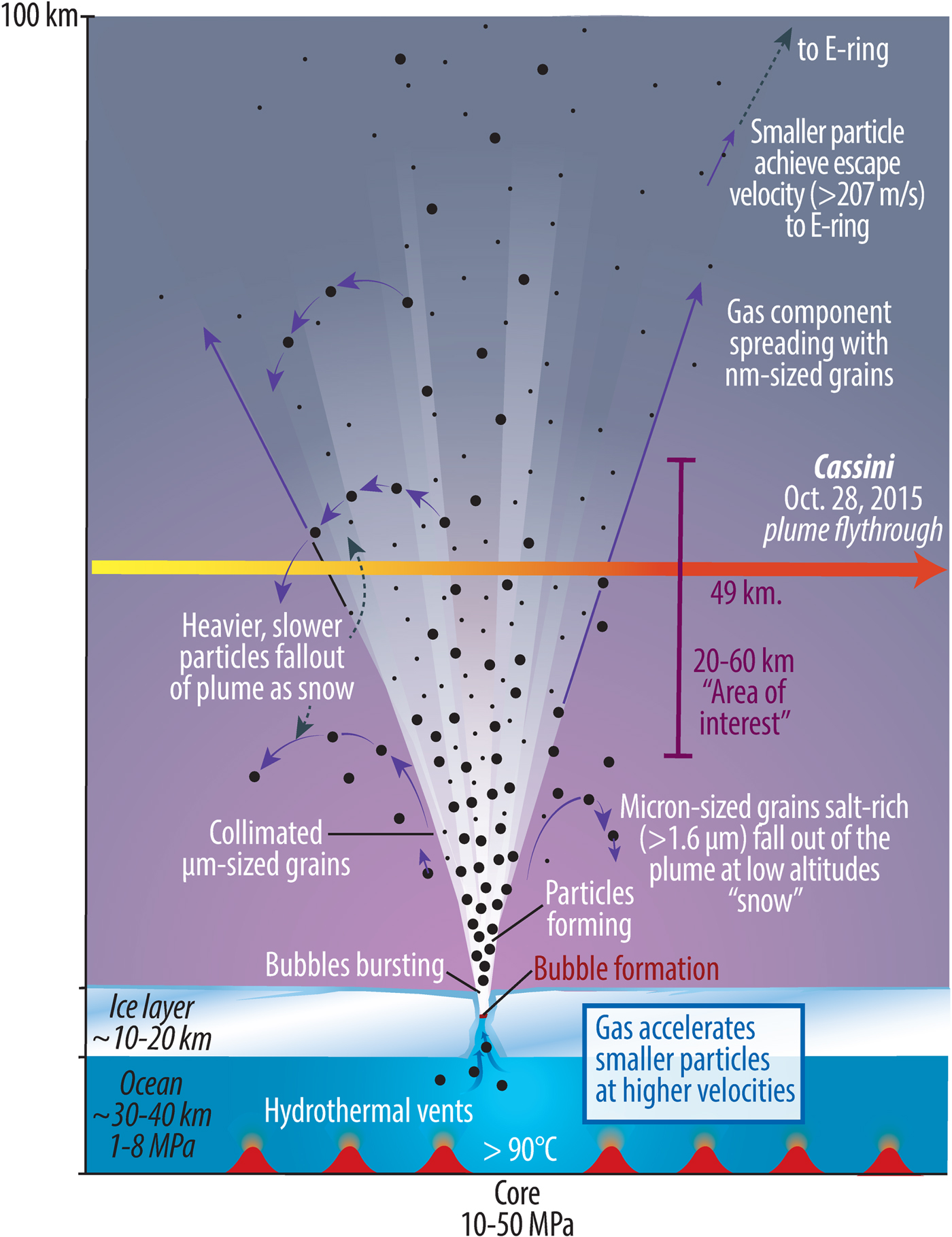
Fig. 1. Cross-section view of Enceladus tiger stripe vent. Not to scale.
We develop a physics-based plume model and fit that model to results from Porco et al. (Reference Porco, Dones and Mitchell2017b). This model folds together observations of (a) the size distribution of erupted ice particles, with (b) the total mass flux being erupted, and (c) the location and geometry of the eruptive sources. We assume a ‘nominal model’ based on our fits to Cassini data and use those nominal conditions to assess captured sample mass as a function of altitude as shown in Fig. 2. We choose a viable ‘area of interest’ for a collection that is <60 km based on the sharp decrease in plume density above this altitude.
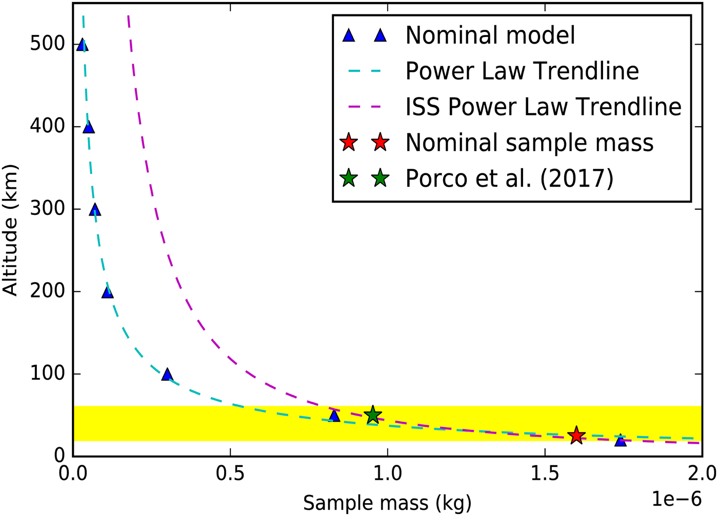
Fig. 2. Nominal model results for sample mass versus altitude (triangles) with a power law function fit (dotted line) and a nominal sample mass estimate based on the fit to ISS observations (Porco et al. Reference Porco, Dones and Mitchell2017b) is marked with a star. The highlighted region shows the ‘area of interest’ for collection from 20 to 60 km above the Enceladus surface. Here we show a single sample mass, altitude point (~1E-6, 50) fit to an early brightness versus altitude curve published by Schmidt et al. (Reference Schmidt, Brilliantov, Spahn and Kempf2008) in that paper's Fig. 3. More comprehensive, but unpublished, ISS brightness versus altitude curves for multiple flybys show even better agreement to our results.
The initial conditions for the dust in our model are based on observations and observationally-derived values from the Cassini ISS instrument (Porco et al. Reference Porco, Dones and Mitchell2017b). Our modelling results are in agreement with the results of related models (Kempf et al. Reference Kempf, Beckmann, Moragas-Klostermeyer, Postberg, Srama, Economou, Schmidt, Spahn and Grün2008; Schmidt et al. Reference Schmidt, Brilliantov, Spahn and Kempf2008; Postberg et al. Reference Postberg, Schmidt, Hillier, Kempf and Srama2011). Initial conditions of the particles are (Vi, S i) for the 100 + jets. Furthermore, the nominal model assumes the initial conditions shown in Table 1.
Table 1. Nominal plume model geophysical parameters

Free parameters matched to observational Cassini instrument results.
a q = 4 is chosen as nominal versus q = 3 as it allows better agreement with CDA and RPWS, with respect to the constraints CDA has put on the total particulate mass rate (Schmidt et al. Reference Schmidt, Brilliantov, Spahn and Kempf2008) and constraints CDA and RPWS have put on impact rates (Ye et al. Reference Ye, Gurnett, Kurth, Averkamp, Morooka, Sakai and Wahlund2014)
The plume model spacecraft parameters are summarized in Table 2. A given spacecraft ephemeris (θ, ϕ, r) is fed into the simulation. This allows for a variable spacecraft altitude in relation to the Enceladus ground. This capability is necessary in order to validate the model against existing Cassini data sets, e.g. a correlation to the CDA E7 pass seen in Fig. A4. For the purposes of mass interception and amino acid results shown in this paper, we assume a constant altitude above the surface of Enceladus.
Table 2. Plume model spacecraft parameters

A key new effort of this work is to computationally model grain densities at lower altitudes than Cassini flight paths while simultaneously fitting the results of the model to Cassini datasets at higher altitudes. For a given spacecraft position (θ, ϕ, r) a ‘shooting’ method is used to find particles with (Vi, S i) that intersect the spacecraft collector and are solutions by iterating on the second-order ODE for particle trajectories using Runge–Kutta–Fehlberg (RKF) iteration. After the shooting method is used for a single jet and a single collector position, the mass intercepted by the collector is calculated for that jet and position.
Based on the initial conditions of our nominal model, we calculate a nominal sample volume of 1600 µg with a 1 m2 collector in a single pass over the south pole at a 25 km closest approach altitude. Figure 3 shows an example of model output where jets ‘tagged’ with green dots are those jets which contribute material to the overall collection by the spacecraft collector. Additional descriptions of the numerical methods used in the computational plume model are found in the Appendix Section.

Fig. 3. Example of output of encountered jets ‘tagged’ with green dots for a given spacecraft ground-track. Note for the jet configuration some jets even close to the ground-track will not contribute to the total mass collection, due to high zenith and azimuth tilts, as well as narrow spread angles which cause the spacecraft to ‘miss’ the jet source at low altitudes. The jet source locations shown as green or red dots in this image come from Porco et al. (Reference Porco, DiNino and Nimmo2014). Note that curtain sources along the tiger stripes are not shown in this graphic.
Cometary model and biological model for Enceladus
Low molecular weight organic compounds and inorganic salts are known to be present in the plume of Enceladus based on Cassini results (Waite et al. Reference Waite, Lewis, Magee, Lunine, McKinnon, Glein, Mousis, Young, Brockwell, Westlake, Nguyen, Teolis, Niemann, McNutt, Perry and Ip2009; Postberg et al. Reference Postberg, Schmidt, Hillier, Kempf and Srama2011). Biomolecules, especially amino acids and lipids, are expected to be present as they are found in carbonaceous meteorites or are likely to be a product of any biological process.
Cassini's INMS detected organics over the mass range up to 99 amu (Waite et al. Reference Waite, Combi, Ip, Cravens, McNutt, Kasprzak, Yelle, Luhmann, Niemann, Gell, Magee, Fletcher, Lunine and Tseng2006) and with a resolution of m dm−1 of 100 (Waite et al. Reference Waite, Young, Cravens, Coates, Crary, Magee and Westlake2007) in a series of plume encounters. Based on improved results from the favourable geometry of the E5 encounter, Waite et al. (Reference Waite, Lewis, Magee, Lunine, McKinnon, Glein, Mousis, Young, Brockwell, Westlake, Nguyen, Teolis, Niemann, McNutt, Perry and Ip2009) suggested that many of the volatile compounds in the plume were present at roughly the ratio relative to water seen in comets. In particular, Waite et al. (Reference Waite, Lewis, Magee, Lunine, McKinnon, Glein, Mousis, Young, Brockwell, Westlake, Nguyen, Teolis, Niemann, McNutt, Perry and Ip2009) show that the abundances of CO2, CH4, C2H2, NH3 and H2CO (relative to H2O) in the plume resemble those in comets. They also suggest that CH3CHO and HCN are somewhat elevated in the plume compared with comets while H2S and CH3OH abundances are significantly lower. The comet model for the plume of Enceladus is also explored in McKay et al. (Reference McKay, Khare, Amin, Klasson and Kral2012) and Bouquet et al. (Reference Bouquet, Mousis, Waite and Picaud2015).
Thus the most parsimonious explanation for the rich organic content of the plume of Enceladus is a cometary endowment of organics during planetary accretion. The expectation from this explanation is that biomolecules would have the same concentration in the plume as in comets. With the recent exception of glycine (Altwegg et al. Reference Altwegg, Balsiger, Bar-Nun, Berthelier, Bieler, Bochsler, Briois, Calmonte, Combi, Cottin, De Keyser, Dhooghe, Fiethe, Fuselier, Gasc, Gombosi, Hansen, Haessig, Jäckel, Kopp, Korth, Le Roy, Mall, Marty, Mousis, Owen, Rème, Rubin, Sémon, Tzou, Hunter Waite and Wurz2016), amino acids have not been measured in cometary refractory materials. However, there is evidence that cometary refractory organics are approximated by meteoritic refractory organics. Cody et al. (Reference Cody, Heying, Alexander, Nittler, Kilcoyne, Sandford and Stroud2011) investigated molecular spectroscopic characteristics of organic solids in carbonaceous chondritic meteorites, interplanetary dust particles collected on Earth, and Comet 81P/Wild 2 particles returned by the Stardust mission. They conclude that their results support the hypothesis that chondritic insoluble organic matter (IOM) and cometary refractory organic solids are related chemically and likely were derived from formaldehyde polymer. Fray et al. (Reference Fray, Bardyn, Cottin, Altwegg, Baklouti, Briois, Colangeli, Engrand, Fischer, Glasmachers, Grün, Haerendel, Henkel, Höfner, Hornung, Jessberger, Koch, Krüger, Langevin, Lehto, Lehto, Le Roy, Merouane, Modica, Orthous-Daunay, Paquette, Raulin, Rynö, Schulz, Silén, Siljeström, Steiger, Stenzel, Stephan, Thirkell, Thomas, Torkar, Varmuza, Wanczek, Zaprudin, Kissel and Hilchenbach2016) report on the analysis of solid organic matter in the dust particles emitted by comet 67P/Churyumov– Gerasimenko and suggest that it is analogous to the IOM found in the carbonaceous chondrite meteorites. They conclude that the observed cometary carbonaceous solid matter could have the same origin as the meteoritic insoluble organic matter, but suffered less modification before and/or after being incorporated into the comet.
Following this logic, we assume cometary carbonaceous solid matter and meteoritic IOM are equivalent and we chemically model Enceladus as a comet. Thus we suggest the simplest approach to estimating biomolecules in the ocean of Enceladus is to assume that Enceladus has the organic composition of comets – from which it formed – and that we can estimate the expected amino acid concentrations and distribution from meteoritic organic matter. The organic content of the refractory organic material in carbonaceous chondrite meteorites has been measured in detail (e.g. Glavin et al. Reference Glavin, Callahan, Dworkin and Elsila2011). The simplest amino acid, glycine, is present from 1–50 ppm; for reference, the Murchison meteorite has a concentration of 2 ppm glycine.
Based on this approach we can estimate the glycine content in the ocean by scaling to the total organic content observed in the plume. Based on Cassini results (INMS) we estimate the total organic content of the ocean as 0.01–0.1%. The total organic content in carbonaceous meteorites is ~2%. Proportional scaling thus gives a glycine concentration in the ocean of Enceladus of 0.005–2.5 ppm.
We note that Altwegg et al. (Reference Altwegg, Balsiger, Bar-Nun, Berthelier, Bieler, Bochsler, Briois, Calmonte, Combi, Cottin, De Keyser, Dhooghe, Fiethe, Fuselier, Gasc, Gombosi, Hansen, Haessig, Jäckel, Kopp, Korth, Le Roy, Mall, Marty, Mousis, Owen, Rème, Rubin, Sémon, Tzou, Hunter Waite and Wurz2016) reported on the direct detection of glycine in comet 67P/Churyumov-Gerasimenko by Rosetta by the analysis of small discrete particles. Some particles had no glycine (presumably pure water) and some had 0.16% glycine. Some considerable uncertainty remains in the bulk abundance in comets given the small number of samples, but the range of values (0–1600 ppm) is certainly consistent with the analysis above.
As an interesting alternative to the comet model, we consider Earth's deep ocean. Hence, for estimating the amino acid concentration in the ocean of Enceladus, another possible analog is the deep ocean waters of Earth. Although the physical and any biological processes operating in the ice-covered ocean of Enceladus are different than on Earth the analog is broadly suggested and may be quite useful given the precise measurements of the amino acid concentration in Earth's oceans. It provides a defined biological case to consider.
The amino acids in the ocean are present in free and combined form (e.g. Sommerville & Preston Reference Sommerville and Preston2001). Combined amino acids are various compounds including proteins and peptides, proteins linked to sugars and amino acids adsorbed to humic and fulvic acids, clays and other materials. Several studies (e.g. Lee & Bada Reference Lee and Bada1977) indicate that in the deep ocean the dissolved free amino acid concentration is ~40 nM and the dissolved combined amino acid concentration is ~150 nM. The particular amino acids that dominate in aquatic ecosystems have been tabulated by Moura et al. (Reference Moura, Savageau and Alves2013). Their results for the five amino acids with the highest concentration, making up 64% of the total, are given in Table 3.
Table 3. Five most common amino acids in aquatic ecosystems (Moura et al. Reference Moura, Savageau and Alves2013)

Combining the total amino acids in the ocean of 190 nM with the fractions in Table 3 gives nominal concentrations on the biotic amino acids listed in Column 3 of Table 3. We use these nominal concentrations in the Results/discussion section to calculate expected concentrations of amino acids in a biotic case.
Spray and ocean composition
Any near-term mission to Enceladus conducting in situ analysis or collecting material for return to Earth is likely to be sampling the spray of ice particles in the plume. A key question is a relationship between the composition of the spray particles and the composition of the ocean. From studies of ocean spray on Earth, it is known that there can be significant differences between the spray and the ocean. The relevance of this phenomenon to Enceladus was pointed out by Porco et al. (Reference Porco, Dones and Mitchell2017a) primarily with respect to microorganisms. We follow that approach with a focus on amino acids.
In Earth's ocean, there has been a considerable study of the process of ‘bubble scrubbing’ where as bubbles rise through water, they scrub the water column so that organisms and organic materials become concentrated on the bubble surface. Figure 4 shows the bubble-related processes that affect the relative concentration of salts, organics and microorganisms, if any, in the plume particles compared with the bulk ocean. As the bubble surface meets the air–water interface at the ocean surface, a thin film forms between the entrapped vapour inside the bubble and the ambient vapour above. As the film thins and then breaks, droplets are produced and expelled upwards. These droplets are called film droplets. Finally, the now-broken bubble results in a central rise of fluid where the burst took place. This fluid peak separates into droplets which are called jet droplets. The jet droplets are generally larger in size than the film droplets. When the bubbles burst, as in ocean spray or in Enceladus's jets, they could eject microbes or biomolecules in the spray. If life exists on Enceladus, the particles in the plume may contain a greater concentration of organisms than the rest of its ocean and/or a higher concentration of organic macromolecules. We consider this bubble ‘enhancement factor’ (EF) in our estimates for the concentration of amino acids in a given sample volume collected in the Enceladus plume.
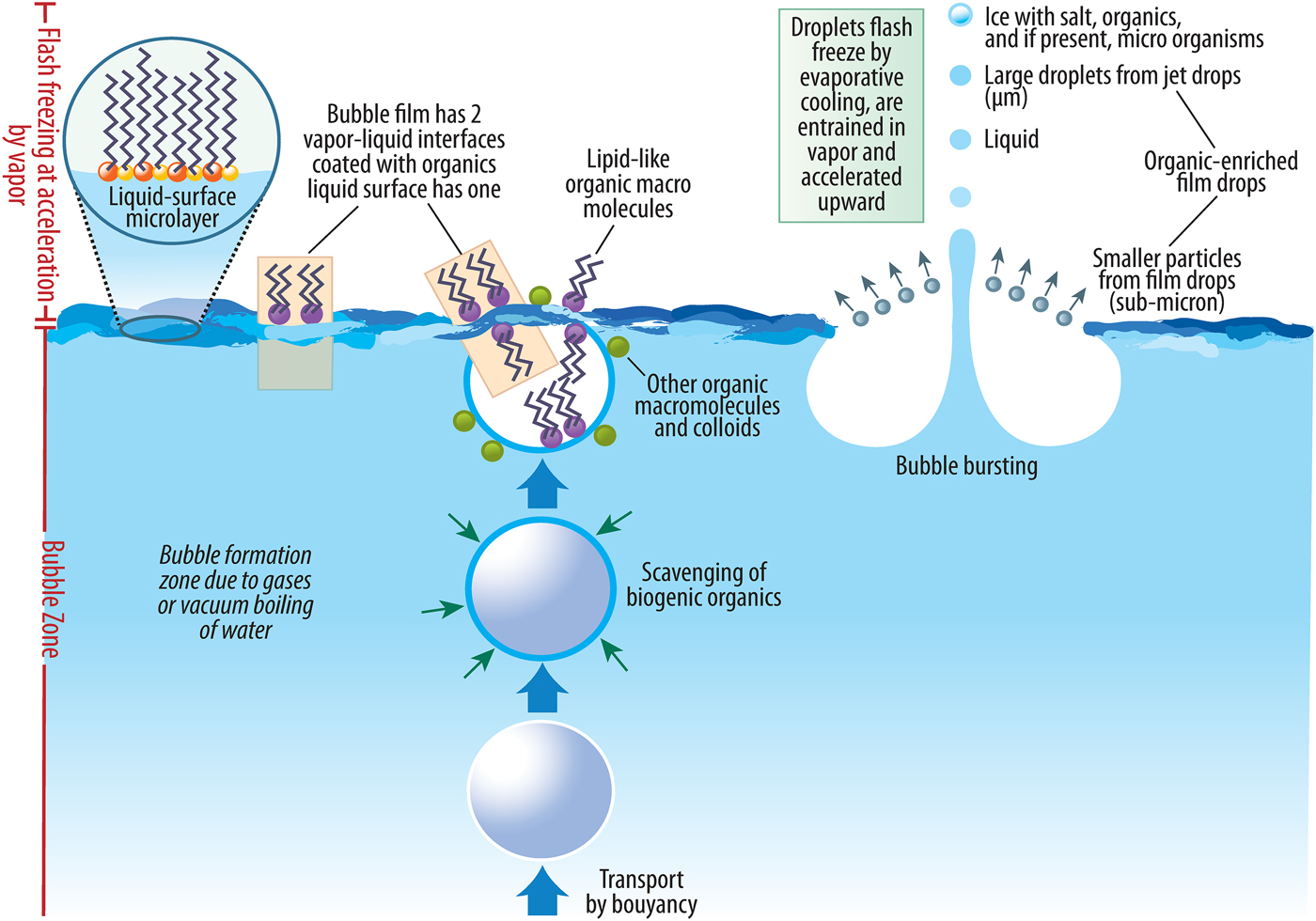
Fig. 4. Zone of bubble formation, bubble bursting and particle formation.
It is important to note, as summarized in Porco et al. (Reference Porco, Dones and Mitchell2017a), that the EF can vary by orders of magnitude and can be dependent on many factors including but not limited to ocean composition, surface properties, morphology (size, shape), the health of an organism, and environmental factors such as temperature and inorganic content (e.g. salinity). Other secondary characteristics also affect how efficiently matter and microbes will attach to rising bubbles, such as how much material is already present, how long it takes the material to attach (related to its surface chemistry) compared with the time it takes it to slide off the interface and back into the bulk fluid, the length of time the bubbles rise through the column, whether or not the saturation limit has been reached and the bulk concentration of the water. As stated in our Introduction, salts and even organics are present in Enceladus particles (Postberg et al. Reference Postberg, Kempf, Schmidt, Brilliantov, Beinsen, Abel, Buck and Srama2009) which also enhances attachment and increases the EF. The longer a bubble ascends, the more matter and microbes it will adsorb. In an environment such as the jet sources on Enceladus, we could expect the biggest drops, which are likely to be jet drops from the largest bubbles, to have the greatest concentration of bacteria, but film drops to be more numerous if bubble sizes are big enough to create them (Porco et al. Reference Porco, Dones and Mitchell2017a). This thinking adds credence to the idea that larger grain sizes, found at lower altitudes, may carry greater concentrations of biomolecules such as amino acids.
If the bulk water is not pure but contains concentrations of either inorganic or organic matter, including amino acids, these can become attached to the vapour–water interface of the bubble as it rises. Whether or not this occurs depends primarily on the solubility of the material and its surface activity; i.e., how it affects the surface tension of the bubble (Porco et al. Reference Porco, Dones and Mitchell2017a).
At the moment of their production, terrestrial film and jet drops have a chemical composition and pH close to that of normal seawater; the fresh sea-salt aerosols inherit these. The ratios of the major seawater ions are preserved in the newly formed aerosols (Warneck Reference Warneck1988). Sea-salt aerosols are alkaline with pH about 7.0 to 8.7 (Keene & Savoie Reference Keene and Savoie1998) compared with the ocean pH of 8.1. A specific feature of the fresh sea-salt aerosols, transferred to aged sea-salt aerosols, is their enrichment with organic matter (Blanchard Reference Blanchard1982; Middlebrook et al. Reference Middlebrook, Murphy and Thomson1998), iodine (Cicerone Reference Cicerone1981; Murphy et al. Reference Murphy, Thomson and Middlebrook1997) and even live organisms and bacteria (Blanchard & Syzdek Reference Blanchard and Syzdek1972, Reference Blanchard and Syzdek1982).
Kuznetsova et al. (Reference Kuznetsova, Lee and Aller2005) empirically measured concentrations of dissolved free (DFAA), dissolved combined (DCAA) and particulate amino acids (PAA) in natural and simulated aerosols on Earth. This study was based on the terrestrial understanding that marine aerosols transfer oceanic material to the atmosphere. Most of this marine aerosol originates when bubbles burst at the ocean surface and eject material from the liquid-surface microlayer and bubble surface layers into the air. They found that surface layer concentration of chemical compounds such as amino acids often differed from bulk water concentrations. According to their results, DFAA and DCAA enriched the aerosols sampled by 1–8.2× and 2–8.4×, respectively, compared with bulk seawater. PAA enhancement was usually higher (up to 50-fold). We use these enrichment factors for amino acids in our calculations in the Results/discussion section.
We acknowledge future work should consider other processes besides bubble bursting. For example, the R −4 aspect of the plume particle size distribution suggests a ‘fluidization’ near the vent where the particulates are of such high number density they are collisional near the fissure (e.g. Yeoh et al. Reference Yeoh, Li, Goldstein, Varghese, Levin and Trafton2016), creating smaller fragments and also a fractal-like particle size distribution with many small and progressively fewer large particles. This could be similar to the ‘saltation’ layer formed at the bottom of a dust devil (Kok et al. Reference Kok, Parteli, Michaels and Bou2012). In Earth's ocean, bubbles form and move vertically via passive buoyant forces, or adiabatic processes. In the Enceladus plume, the jet sources are under a strong head pressure forcing the fluid out so the process is not adiabatic. It is unclear if a bubble can form and remain stable in the flow, since the flow may break up the bubble before it reaches the surface due to hydrodynamic instability. A future laboratory study may be to examine a liquid–vacuum interface with liquid under pressure and consider the Joule-Thomson effect where there is a spray and the transition to a head pressure to a vacuum creates droplets.
Results/discussion
For the abiotic case, we take the organic content of the refractory organic material in meteorites, specifically of the Murchison meteorite, scale the amino acid content to the total organic content observed in the Enceladus ocean (Waite et al. Reference Waite, Lewis, Magee, Lunine, McKinnon, Glein, Mousis, Young, Brockwell, Westlake, Nguyen, Teolis, Niemann, McNutt, Perry and Ip2009), and extract an amino acid concentration in the Enceladus ocean. Proportional scaling thus gives a glycine concentration in the ocean of Enceladus of 0.005–2.5 ppm. We have used the relative abundances of the other amino acids against glycine. An important note is that while we have used the relative abundances of the other amino acids against glycine in the Murchison meteorite, meteorite content can vary significantly based on the given meteorite, e.g. Fig. 4 in Glavin et al. (Reference Glavin, Callahan, Dworkin and Elsila2011).
In the biotic case, we use the terrestrial deep ocean case and assume ~190 nM total amino acids. We combine the total amino acids in the ocean with the fractions given in Table 3 to predict nominal concentrations of biotic amino acids in an Enceladus sample.
Combing the mass collection with the abiotic and biotic models allows us to compute the expected mass of amino acids collected in a plume pass through. For item j this mass, M j is given by
 $$\eqalign{ M_{\rm j}\, = \,&{\rm mass}\,{\rm collected} \times {\rm concentration}\,{\rm in}\,{\rm the}\,{\rm ocean} \cr &\times {\rm spray}\,{\rm enhancement}\,{\rm factor}}$$
The amino acid EF range is taken to be a midpoint value of 4.6 for DFAA, 5.1 for DCAA and to be 50 for PAA (Kuznetsova et al. Reference Kuznetsova, Lee and Aller2005). The nominal sample mass used here is 1600 µg per Fig. 2. Table 4 shows the expected amount of intercepted amino acids for the abiotic and the biotic model for the Enceladus ocean.
Table 4. Mass of amino acids in the intercepted sample for a 1 m2 collector on a spacecraft with the closest approach of 20 km during mean plume activity for the given nominal particle size distribution, n(R) ~ R −4

Conclusion
There is every indication that the ocean on Enceladus is habitable and that the icy particles in the plume are samples of that habitable water. This motivates future missions to collect these icy grains and search for signs of life. Given the uncertainties regarding the conditions under which life originates, the most conservative hypothesis for Enceladus is that organic matter in the ocean reflects purely abiotic sources and the resulting organic pool resembles the organic composition observed in meteorites, comets and abiotic hydrothermal simulations. In order to go further and identify possible biological cases, future missions will need to target certain diagnostic compounds such as amino acids and lipids. Here we present expected amino acid concentrations in the Enceladus plume based on estimated sample mass at low altitudes and enhancement factors due to the phenomena of bubble scrubbing.
Appendix: Collecting amino acids in the plume of Enceladus
This Appendix describes the computational geophysical model used to ascertain mass sample as a function of altitude in the Enceladus plume. We use results from this model, which is derived from Cassini observations, to quantitatively estimate amino acid concentrations available for interception by a spacecraft.
Nominal model
In this section, we describe our numerical dust model and its nominal parameters. The nominal model has been formulated based on direct observations or a fit to direct observations from the Cassini Imaging Science Subsystem (ISS) and the CDA-High Rate Detector (CDA-HRD). The numerical dust model decomposes the Enceladus plume into the ~100 individual jets identified by Porco et al. (Reference Porco, DiNino and Nimmo2014) and putative interjet material, each of which launches a population of particles with a size-dependent launch velocity distribution and tracks their motion under Enceladus's gravity. After exiting the surface sources, gas drag, other gravity terms and electrostatic forces are not significant for the largest (>0.01 µm) particles which we choose to selectively model here. Thus, particle motions are purely ballistic,
 $$\displaystyle{{d{\bi V}} \over {dt}} = - {\bi g}\left( {\displaystyle{1 \over {r^2}}} \right)$$
Nominal initial conditions of the dust
The initial conditions for the dust are based on observations and observationally-derived values from the Cassini ISS instrument (Porco et al. Reference Porco, Dones and Mitchell2017b). Full model initial parameters are detailed in Table 1 in the main text. Additional details of the model's initial conditions are below.
Source geometry
The starting positions are the ‘tiger stripes’ and ~100 jet locations (Porco et al. Reference Porco, DiNino and Nimmo2014) on Enceladus's south polar region. The jet locations are modelled as point sources. The quasi-continuous emission from the tiger stripes is mimicked by equidistant point source locations along each stripe to simulate curtain sources. A jet source is defined by locations given by Porco et al. (Reference Porco, DiNino and Nimmo2014) and has a slimmer spread angle as well as a higher mass production rate. A tiger-stripe source is defined as interjet material placed continuously along the tiger stripes to simulate ‘curtains’ (Spitale et al. Reference Spitale, Hurford, Rhoden, Berkson and Platts2015). This interjet material is given a wider spread angle and a lower particulate mass rate in order to simulate the ‘continuum’ of material measured by instruments such as the CDA and the RPWS (Meier et al. Reference Meier, Kriegel, Motschmann, Schmidt, Spahn, Hill, Dong and Jones2014).
Grain starting directions
The spread angle of an individual jet source and a tiger stripe source, respectively, are 15° and 70°. We choose starting ejection angles which are more diffuse for the tiger stripes and more collimated for the jet sources as has been done in other models to fit Cassini data (Postberg et al. Reference Postberg, Schmidt, Hillier, Kempf and Srama2011; Meier et al. Reference Meier, Kriegel, Motschmann, Schmidt, Spahn, Hill, Dong and Jones2014).
Grain starting velocities
We model particle velocities ranging from 0 to 350 m s−1 using exit velocities from the model of Degruyter & Manga (Reference Degruyter and Manga2011). They consider two alternatives to the model of particle acceleration in the vent: drag-limited and collision-limited acceleration, which link particle size to exit velocity. We have considered both, but present results for the collision-limited model here because this gives the best agreement with the constraints on the size of erupted particles from VIMS and CDA. The collision-limited model is stochastic, i.e. the velocity a particle can reach is not uniquely determined but can be described by an average with a standard deviation for a given radius and vent condition. The Degruyter & Manga (Reference Degruyter and Manga2011) model qualitatively predicts similar results to the modeling by Schmidt et al. (Reference Schmidt, Brilliantov, Spahn and Kempf2008). It is consistent with the observations of particle size on the surface inferred from modelled VIMS data, the size of particles observed with the CDA and VIMS instruments at heights of Cassini flybys and the size of particles that reach escape velocity and are found in Saturn's E ring. We use the exit velocities shown in Fig. 1 of Degruyter & Manga (Reference Degruyter and Manga2011) as starting velocities for our ballistic particles.
Grain initial particle size distribution
The distribution of number density as a function of particle radius is given by a power law, n(R) ~ R − q with q = 4. The distribution of mass as a function of radius is given by N(R) · R 3. This function is then normalized such that it has an integral of one. Because of the normalization, the constant factor of 4/3 πρ is omitted from the calculation.
The Cassini CDA data (Schmidt et al. Reference Schmidt, Brilliantov, Spahn and Kempf2008; Kempf et al. Reference Kempf, Beckmann and Schmidt2010; Postberg et al. Reference Postberg, Schmidt, Hillier, Kempf and Srama2011) and RPWS data (Ye et al. Reference Ye, Gurnett, Kurth, Averkamp, Morooka, Sakai and Wahlund2014) both suggest a power law exponent with q = 3 to 4, and a maximum particle size of 10 µm. The maximum particle size must be due to the physical processes which produce the particles at the water–gas interface; it is not the result of gravity, e.g. Lorenz (Reference Lorenz2015). The lower limit on the particle size is harder to constrain but data from the CDA and RPWS suggests that the mass contribution of particles below 0.2 µm drops significantly.
Unfortunately, there is no upper size limit directly indicated by in-situ measurements. The non-detection of large particles is consistent with a power law of q = 3.5 or steeper. There is most likely an upper size limit for particles in the vents, arising from the condensation physics, the enthalpy of the reservoir and the number density and size-distributions of droplets above the ocean. That upper size limit is not seen in the plume at Cassini flyby altitudes because of the size-dependent ejection velocity (the largest particles do not reach high altitudes or escape velocity to the E ring).
There is also no upper size limit inferred from ISS observations. Porco et al. (Reference Porco, Dones and Mitchell2017a, Reference Porco, Dones and Mitchellb) inverted ISS images taken at high phase angle at many points in Enceladus's orbit. They found that a power law fits the data with values of q = 3–4. The ISS inversion integrates over particles from 0.01 to 10 µm but in practice, only a subset of these contribute to the ISS signal. The limits of that subset depend on the q value, the 5% and 95% cumulative values are for q = 3, 0.27–8.0 µm. (i.e. the ISS inversion is only 10% sensitive to any particles outside this size range) and for q = 4, 0.14–2.8 µm. Therefore, Porco et al. (Reference Porco, Dones and Mitchell2017b) cannot constrain R max at all due to the sensitivity of the instrument.
Total particulate mass rate
Our nominal total particulate mass rate is 16 kg s−1 based on a fit to the power law exponent and particle range chosen by Porco et al. (Reference Porco, Dones and Mitchell2017b). In the modelling, the total mass of all ejecta from Enceladus (16 kg s−1) is split among both the 100 jet sources and 400 created curtain sources. 80% of the mass (12.8 kg s−1) is split evenly among each of the jet sources (0.128 kg s−1 to each jet source) and the remaining 20% of mass (3.2 kg s−1) is split evenly amongst the 400 created curtain sources or .032 kg s−1 given to each curtain source. Each source's allotted mass flux is then distributed across grain sizes for the individual particles. This mass distribution fits best with available CDA-HRD E7 data and multiple ISS observational data sets, but the mass distribution across individual jet and curtain sources is an area for additional exploration. In fact, the mass rate most likely varies across individual jet and curtain sources (Kempf et al. Reference Kempf, Beckmann and Schmidt2010).
Spacecraft Ephemeris
The plume model spacecraft parameters are summarized in Table 2 in the main text. A given spacecraft ephemeris (θ, ϕ, r) is fed into the simulation. This allows for a variable spacecraft altitude in relation to the Enceladus ground. This capability is necessary in order to validate the model against existing Cassini data sets, e.g. a correlation to the CDA E7 pass. For the purposes of mass interception and resulting amino acid results shown in this paper, we assume a constant altitude above the surface of Enceladus. In all calculations, we use the Enceladus radius at the south pole, considering also the 500–1000 m depression of the south polar terrain.
Analytical starting point
Analytical extrapolation from Cassini literature
We use published particle densities from the literature (e.g. Dong et al. Reference Dong, Hill and Ye2015) to analytically predict the intercepted sample along the Cassini flight paths. Dong et al. (Reference Dong, Hill and Ye2015) fit their results to the Cassini Plasma Spectrometer (CAPS) and the RPWS results. The analytical mathematical approach described below is also used for the computational modelling.
The geometry and motion of the collector are shown in Fig. A1. We assume the collected sample mass is
 $${\rm mas}{\rm s}_{{\rm Acc}} = r(r){\rm} ({\bf A}^.{\bf v})t\ $$
where t is the time spent in the plume collecting, and is equal to the path length through the plume, L, divided by the spacecraft ram speed, v ram:
 $$t = L/v_{{\rm ram}} $$
The vector dot product A·v includes the collection components. The velocity vector is the addition of the ram vector component and average speed of the plume component. Generally, v = vram + vplume, so that
 $${\rm A}{\bf n}^.\,{\bf v} = {\rm A}{\rm v}_{{\rm ram}}{\rm cos}\left( {{\rm q}_{{\rm ndotvram}}} \right) + {\rm A}{\rm v}_{{\rm plume}}{\rm cos}\left( {{\rm q}_{{\rm ndotvplume}}} \right)$$
while V ram and V plume are not necessarily always perpendicular to each other, if we assume this scenario, then
 $${\rm 9}0^{\rm o} = {\rm \theta }_{{\rm ndotvram}} + {\rm \theta }_{{\rm ndotvplume}}$$
Thus, making cos(θndotvplume) = sin(θndotvram). We can call this a ‘quasi-perpendicular’ scenario:
 $${\rm A}{\bf n}^.\,{\bf v}\ \sim{\rm A}{\rm v}_{{\rm ram}}{\rm cos}({\rm \theta} _{{\rm ndotvram}}) + {\rm A}{\rm v}_{{\rm plume}}{\rm sin}({\rm \theta} _{{\rm ndotvram}}) $$
Combining (A1), (A2) and (A3) we find
 $${\rm Mas}{\rm s}_{{\rm Acc}} = {\rm \rho} \left( r \right){\rm L A} [{\rm cos}({\rm \theta} _{{\rm ndotvram}}) + v_{{\rm plume}}{\rm sin}({\rm \theta} _{{\rm ndotvram}})/v_{{\rm ram}}] $$
We note the general trend that when the ram speed is very fast compared with the plume particle speed, v ram >> v plume the first term in the brackets dominates and becomes its largest value by a collector oriented in the ram direction (θndotram = 0o). In contrast, if a craft passes very slow or hovers over the plume such that v ram < v plume, then the second term in the brackets dominates and becomes its largest value for a nadir-pointing collector (θndotram = 90o).
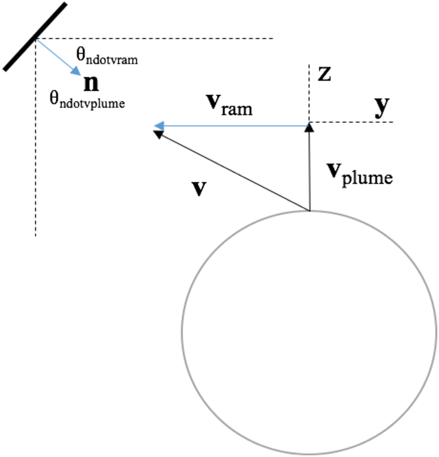
Fig. A1. Illustration of Enceladus plume and collector geometry used in analytical and computational modeling.
Analytical prediction of sample mass
For v ram >> v plume, the second term in brackets in Eq. A4 becomes small and the mass collection is simply a function of the path length ‘plowed’ by a ram-oriented spacecraft collector (θndotvram = 0o). In this case,
 $${\rm Mas}{\rm s}_{{\rm Acc}}\sim{\rm \rho} (z){\rm} L\left( z \right){\rm} A. $$
where L is the path length through the particulate cloud and A = 1 m2 is the ram-directed collector area. Dong et al. (Reference Dong, Hill and Ye2015) calculated the mass density, ρ, for the E17 and E18 plume over-flights at ~75 km altitude to be ~10−11 kg m−3 (Table 4, Dong et al., Reference Dong, Hill and Ye2015). For E17 and E18, the spacecraft spent about 15 s in a region of high particulate density (Fig. 4, Dong et al., Reference Dong, Hill and Ye2015), making the path length of a flythrough L ~ 7.5 km s × 15 s ~ 100 km. Consequently, the mass accumulated is 10−6 kg or ~1000 µg for these two passes at 75 km.
This accumulated mass from this simple approach yields results comparable with our computational modelling results (see Fig. 2 in the main paper). It should be noted that the numerical model and the analytical model are not perfect correlations in their initial assumptions with the overall plume source rate, R, consistent with Eq. (A5) at 75 km being ρ vplume π (L/2)2 ~ 15 kg s−1. We arrived at this rate, R, by estimating the mass flux, ρ vplume, at 75 km passing vertically in bulk at ~200 m s−1 through a circle of L/2 = 50 km radius overtop the plume region.
Computational modelling
Numerical methods
A key new effort of this work is to computationally model grain densities at lower altitudes than Cassini flight paths while simultaneously fitting the results of the model to Cassini datasets at higher altitudes. For a given spacecraft position (θ, ϕ, r) a ‘shooting’ method is used to find particles with (Vi, S i) that intersect the spacecraft collector and are solutions by iterating on the second-order ODE for particle trajectories using RKF iteration.
After the shooting method is used for a single jet and a single collector position, the mass intercepted by the collector is calculated for that jet and position as described below in the next section.
Mass collection
Solutions are found using the RKF solver for a spacecraft position and also a position 1 m above that position. With these solutions acting as streamlines in a fluid flow, as shown in Fig. A2, they bound an amount of mass between them. The amount of mass which is bounded is given by the difference between the initial zenith angle of each particle divided by the jet spread angle. This streamlined area is used to generate a per meter length density (for the line between the 2 points). We assume the density is the same locally and use that density to extrapolate an areal density at the location of the collector (given by the original two positions).

Fig. A2. Cartoon illustrating mass collection calculation in computational plume model where ϕm,ice is the mass flow rate through an area given by the zenith angle solutions.
Then the spacecraft position and velocity is stepped forward in its trajectory using its ephemeris data and the program uses the density profile for a 1 m3 volume in front of the spacecraft collector. The calculated density is multiplied by the volume swept out by the collector between time steps to obtain a mass collection which is added to a mass collection tally. That local density is assumed until the next time step when a new spacecraft position is used to find solutions using the RKF solver and the process is repeated. The simulation outputs the total mass collection as well as the mass attributed to each individual source. We find the mass density in the given volume by multiplying the percentage of the total particulate mass using the chosen possible zenith angles, azimuth angles and initial velocities and at the right time (using average particle velocity near the collector).
What is important for the calculation of particles ‘intercepted’ by the surface of the collector is the relative velocity in the reference frame of the collector; we have expressed it as two components of the mass collection. These two components are mathematically described by the two terms in Eq. (A4). When the velocity of the ice particles is much less than the velocity of the spacecraft the plume can be treated as a ‘static’ plume with a constant density which the spacecraft can sweep through. The particle collector is treated as a 1 m2 flat plate. The orientation of the collector plate is defined in the computational model. A vector normal to the collector surface is defined and the angle between the collector normal vector and a given particle velocity at the moment of impact (between plate and particle) is taken using a dot product to determine the mass flux into the collector.
Summary of model output
A model run consists of the program iterating through each jet for each spacecraft position and identifying those jets which have particles with initial position and velocity solutions to the boundary value problem. Therefore, for each spacecraft position, the program iterates through the 100 jets (or more, given curtain sources), finds which jets can contribute mass at that position and tags them. These tagged jets are marked by green dots, as shown in Fig. 3, at the end of each full simulation run.
A model run generates total mass collection in kg, a list of n number of jets encountered with mass collected from each in kg, density as a function of spacecraft position in kg m−3 versus (θ, ϕ, r) and the particle size distribution of the intercepted mass in kg versus R. This Appendix focuses on reporting mass collection as a function of altitude.
Results
The results of our nominal model and a discussion of perturbations on that nominal model are below.
Nominal model
Our model has several parameters which ideally would be set based on comparison with observation. These are (1) the total mass production rate of particles, (2) the particle size distribution including the upper and lower limits of particle sizes, coupled to the initial velocities of the particles as they exit the source region and (3) the source locations and geometries, e.g. the zenith and azimuth angles of any ‘tilted’ jet sources.
Porco et al. (Reference Porco, Dones and Mitchell2017a, Reference Porco, Dones and Mitchellb) inverted ISS images taken at high phase angle at many points in Enceladus's orbit. They found that a power law fits the data with values of q = 3–4. The ISS inversion integrates over particles from 0.01 to 10 µm but in practice, only a subset of these contribute to the ISS signal. The limits of that subset depend on the q value, the 5% and 95% cumulative values are for q = 3, 0.27–8.0 µm. (i.e. the ISS inversion is only 10% sensitive to any particles outside this size range) and for q = 4, 0.14 –2.8 µm. Porco et al. (Reference Porco, Dones and Mitchell2017a) also determine the column volume of particles in the plume at various altitudes – effectively the volume that a collector would sweep up moving through the plume. Our results, given in sample mass as a function of altitude, are shown in Fig. 2 of our main paper. Given the particle size distribution velocity, we match these column volume amounts by adjusting the mass production rate and initial velocity. We find a fit with a mass rate of 24 kg s−1 when q = 3 and 16 kg s−1 when q = 4. We explain our selection of q = 4 for the nominal model in the next section while discussing the CDA ‘case’.
We fit our 25 km altitude sample mass to Porco et al., (Reference Porco, Dones and Mitchell2017b) results which predict a mean collection of 3600 µg for q = 3 and a mean collection of 1600 µg for q = 4, not accounting for orbital variance in plume brightness. We show fits to the ISS observations at the lower altitudes (20–60 km) which is our ‘area of interest’. Note that the lower limit of the particle size range (0.01 µm) is getting close to the particle range where electrodynamic forces may become important – and this effect will affect the mass sample measurements at higher altitudes more than lower altitudes based on the particle trajectories. Continuing work on this model should include electrodynamics especially if the particle size distribution is continued below 0.01 µm (e.g. Meier et al. Reference Meier, Kriegel, Motschmann, Schmidt, Spahn, Hill, Dong and Jones2014).
Variations from the nominal model: examining non-uniqueness
Our nominal model parameters are described in Table 1. However, we acknowledge that each of the model parameters is widely constrained, unconstrained and/or a topic of debate. As a result, this predictive model is inherently non-unique, especially when considering the actual emission from the fissure source. We have attempted to fit quasi-consistently as many data sets as is available in the literature and final validation of this and other plume models will be made when a spacecraft passes through the plume at low altitudes. In this section, we explore perturbations on the nominal model and explore the effects on sample mass versus altitude due to a variation on several important parameters in Table 1.
Relationship of q and R max
Our first perturbation follows the lack of direct measurement indicating a maximum particle size produced at the Enceladus vents. The CDA instrument senses large particles but cannot separate them discretely by an integer value, and optical methods are not sensitive to the large particles. The CDA-HRD instrument uses four threshold detectors and has directly detected particles greater than (e.g. 6.5 µm) a given grain size (Kempf et al. Reference Kempf, Southworth, Srama, Schmidt and Postberg2016). The ISS and VIMS instruments are not sensitive to large sizes (Hedman, et al. Reference Hedman, Gosmeyer, Nicholson, Sotin, Brown, Clark, Baines, Buratti and Showalter2013; Porco et al. Reference Porco, Dones and Mitchell2017a). Ye et al. (Reference Ye, Gurnett, Kurth, Averkamp, Morooka, Sakai and Wahlund2014) report on the RPWS data and indicated particles larger than the nominal 10 µm reported by them are present. In the Ye et al. (Reference Ye, Gurnett, Kurth, Averkamp, Morooka, Sakai and Wahlund2014) Fig. 7, the peaks at the upper size limit of the histograms indicate clipped signals caused by dust particles larger than the upper size limits of the corresponding gain levels. This indicates that the power law size distribution applies to a wider-size range than the instrument limit.
There is no Cassini data indicating a maximum size of the particles in the Enceladus plume. However, for our nominal model for q = 4 this does not matter much. But if q = 3 this does matter. We take our nominal model (q = 4, R max = 10 µm giving a fitted value of P = 16 kg s−1) and consider the sensitivity of collected mass to changes in R max and q.
We integrate over the differential mass density distribution where A o is a constant chosen as the total mass production, P, and based on our fit to Porco et al. (Reference Porco, Dones and Mitchell2017b).
 $$M\left( R \right) = A_{o}\int_{R{\rm min}}^{R{\rm max}} {n\left( R \right) \cdot} \displaystyle{4 \over 3}\pi R^3\rho \; dR $$
where n(R) = R −q and q = 4 per the nominal model. We plot mass production rate versus R max in Fig. A3 based on Eq. (A6).

Fig. A3. Grain production rate versus R max for different power-law exponent values.
As is clear from Fig. A3 changing R max for the q = 4 Nominal Model has little effect on the collected mass. But if q = 3 there is a lot of mass in the larger particles and analyses based on current instrument limits could underrepresent the total particulate mass rate at the surface.
CDA case
Our nominal model is defined based on the Porco et al. (Reference Porco, Dones and Mitchell2017b) results from ISS observations. However, it is paramount to consider the case of the CDA data, as the CDA instrument cannot only measure impact rates with the CDA-High Rate Detector (CDA-HRD) but also that team has compared their data to a physics-based model which should have similar results to our own.
The CDA is a complex instrument and should really be separated into two different instruments. We rely on a comparison with the HRD here as it is most applicable as a comparison with our model. The probability that a particle of size R contributed to the HRD counts in a plume pass depends on the total volume swept out and the density
 $$N(R) = {\rm integral}\ {\rm over}\ {\rm the}\ {\rm path}\ {\rm of}\ n(R)\ {\rm A\ dl}\ \sim n(R){\rm A} \times {\rm L}$$
There are subtleties and complexities in interpreting the HRD data due to a fairly large minimum detection (~1 µm) and the binning of particles into four mass threshold categories. Turning this data into a mass production rate or mass collection per unit area in a plume pass is highly model dependent in terms of how one devises the particle size distribution.
In Fig. A4 we compare our model to CDA and RPWS dust densities. Using a spectrum of different source geometries, a power law with q = 4 and a mass rate of 2.7 kg s−1 (Kempf et al. Reference Kempf, Southworth, Srama, Schmidt and Postberg2016), we get peak dust densities of 4–17 particles m−3 for R > 1.7 µm particles for the E7 flyby. Our range in dust density correlates to the possible range in predicted source geometries (Porco et al. Reference Porco, DiNino and Nimmo2014; Spitale et al. Reference Spitale, Hurford, Rhoden, Berkson and Platts2015). This is consistent with the CDA peak density of ~9 particles m−3 for the instrument's 1.7 µm threshold. Ye et al. (Reference Ye, Gurnett, Kurth, Averkamp, Morooka, Sakai and Wahlund2014) found consistency between the dust densities from RPWS and CDA for E7, taking into consideration different particle size thresholds and effective impact areas for each instrument.

Fig. A4. (Left) RPWS and CDA dust densities from the E7 flyby (100 km closest approach) as reported by Ye et al. (Reference Ye, Gurnett, Kurth, Averkamp, Morooka, Sakai and Wahlund2014) for particle radius R > 2.2 µm (RPWS) and R > 1.7 µm and R >2.2 µm (CDA); (Right) Dust density for the E7 flyby from our computational model for R > 1.7 µm. In order to fit the CDA/RPWS dust densities for E7, our model uses a power law with q = 4 describing the particle size distribution and a total mass rate of 2.7 kg s−1 (Kempf et al. Reference Kempf, Southworth, Srama, Schmidt and Postberg2016). The blue curve uses the Porco et al. (Reference Porco, DiNino and Nimmo2014) jet locations and zenith/azimuth angles+additional curtain sources along the tiger stripes, while the red curve uses only the Porco et al. (Reference Porco, DiNino and Nimmo2014) jets.
As described, there is no upper size limit inferred from in-situ measurements since the CDA distinguishes only that there is a particle ≥6.5 µm, for example. Understanding the bi-modal or multi-modal size distribution based on different physical mechanisms, especially for larger particles which dominate the mass density, is an area for future work. Comparisons between our model and RPWS and CDA data for a comprehensive set of trajectories will also better constrain the values of mass rate, source geometry and initial grain velocities for the physics model and is an area for future work. In this way, the comparison with ISS observations for our nominal model uses a more comprehensive data set as those results consider multiple Cassini plume flybys (Porco et al. Reference Porco, Dones and Mitchell2017b) across the Cassini mission's 10-year observation of the plume.
Our model also predicts the discrepancies reported by Porco et al. (Reference Porco, Dones and Mitchell2017a) between the ISS and CDA calculations of total mass rate; as we require mass rates of ~2–5 kg s−1 to match the CDA impact rates and mass rates of ~15–25 kg s−1 to match the ISS extrapolated sample volumes. We suspect that a better understanding of R max created at the vent source and propelled to given altitudes in the plume will help in explaining the discrepancy. We continue to explore the concept of R max and its effects on other parameters in the sections below. Our first perturbation discussion emphasizes the importance of stating both the power law exponent used in modelling and the particle size range (e.g. R max) when stating a particulate mass rate, as even a change in the exponent value could yield substantially different mass rates. For example, we assume mass rates of ~2–5 kg s−1 reported from CDA are tagged to particles in the size range ~0.5–10 µm.
Maximum particle size as a function of altitude
Smaller icy particles in the Enceladus plume accelerate more easily by gas expansion, whereas larger particles tend to fall out of the plume at low altitudes; as a result, only 10% of the total mass in micron-sized particles escapes Enceladus (Schmidt et al. Reference Schmidt, Brilliantov, Spahn and Kempf2008). The question of R max depends not only on the vent physics and the formation of particles there, but also on the separation of particles by gravity as slower particles fall back to the surface at lower altitudes.
Vent
A general approach is to model the expanding flow through a converging–diverging nozzle, and to calculate the acceleration of a particle by the drag of the gas, as calculated, for example, for comet jets (Yelle et al. Reference Yelle, Soderblom and Jokipii2004) or Enceladus (Schmidt et al. Reference Schmidt, Brilliantov, Spahn and Kempf2008; Degruyter and Manga Reference Degruyter and Manga2011). However, a much more succinct method, suitable for expansion into a vacuum (as per Lorenz Reference Lorenz2015, Reference Lorenz2016), is to simply consider the energies involved. The energy acquired by the particle during its acceleration by the gas is ~wr 2P t. A particle made of material with density ρ will have a mass ρr 3, and thus equating the kinetic energy at a final speed V we find
 $$V = \left( {\displaystyle{{wP_{t}} \over {r\rho}}} \right)^{0.5}$$
We use this simple formula to estimate the maximum height of a given particle size, and we compare it with the results from a higher fidelity model by Degruyter & Manga (Reference Degruyter and Manga2011) in Fig. A5.
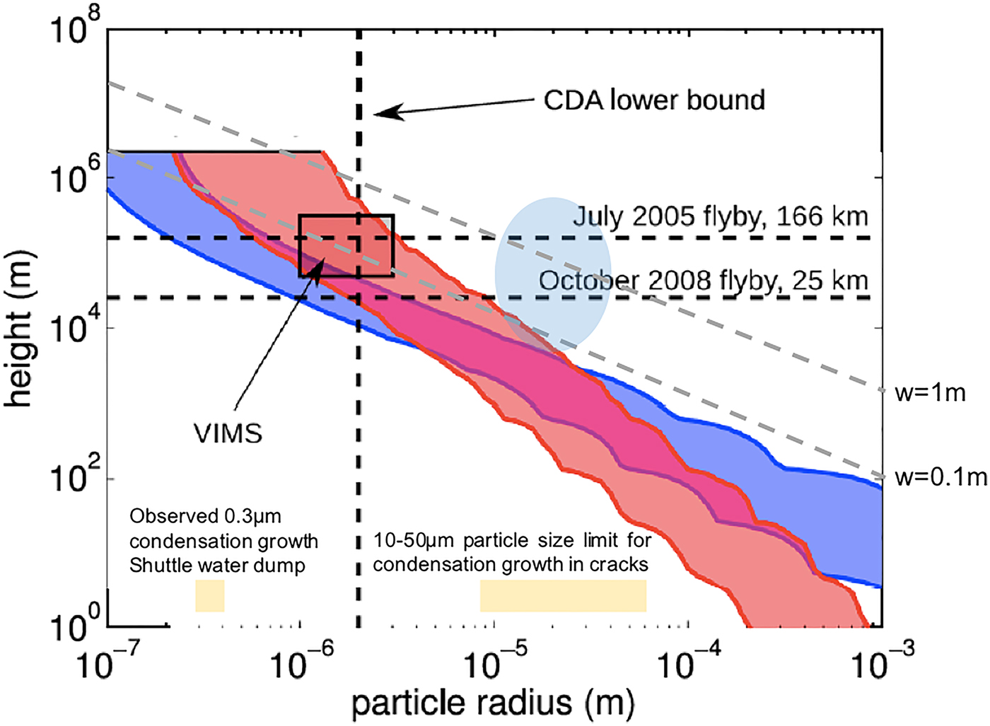
Fig. A5. A modified plot of maximum particle height versus particle radius from Degruyter and Manga (Reference Degruyter and Manga2011). The shaded areas show the solution for a gas temperature range T = 190–273 K using the best fit for the acceleration length of the particles in the subsurface vent. The blue area comes from applying drag-limited acceleration while the red area from applying collision-limited acceleration. The grey dashed lines are from the idealized model of Lorenz (Reference Lorenz2016) assuming a vent crack width of 0.1–1 µm, a throat pressure of 600 Pa and a particle density of 1000 kg m−3. The shaded blue circular region is a statement that for altitudes relevant to this work an R max of 10–50 µm is appropriate. Limits on R max due to studies on condensation growth have been further constrained by the modelling (Schmidt et al. Reference Schmidt, Brilliantov, Spahn and Kempf2008) and in-situ observations of water dumping from the Space Shuttle (Kofsky et al. Reference Kofsky, Rall, Maris, Tran, Murad, Pike, Knecht, Viereck, Stair and Setayesh1992).
In addition to the physics formulation stated above, there are empirical observations and computational modelling which can offer insight on R max. The observation of water dumps from the Space Shuttle estimates a maximum particle diameter of ~500 µm for water at the freezing point (Fowler et al. Reference Fowler, Leger, Donahoo and Maley1990). In further studies of the venting of excess water from the Space Shuttle, Kofsky et al. (Reference Kofsky, Rall, Maris, Tran, Murad, Pike, Knecht, Viereck, Stair and Setayesh1992) find much of the material ends up as 0.3 µm particles from recondensing vapour. For a confined vent system, as in the case of Enceladus, rather than a 2π or 4π expansion from a spacecraft, there is time for particles to grow to the more than a few microns observed by the CDA-HRD. That has been explored by the modelling of Schmidt et al. (Reference Schmidt, Brilliantov, Spahn and Kempf2008) where a 10–50 µm particle size limit was found for condensation growth in the South Polar Terrain vent cracks.
Gravity
Degruyter & Manga (Reference Degruyter and Manga2011) consider two alternatives to the model of particle acceleration in the vent: drag-limited and collision-limited acceleration, which link particle size to exit velocity. They plot maximum particle size versus altitude based on their calculated particle exit velocities (Fig. A6). Ye et al. (Reference Ye, Gurnett, Kurth, Averkamp, Morooka, Sakai and Wahlund2014) reported on the RPWS data and indicated particles larger than the nominal 10 µm reported by them were present during the E7 flyby with the closest approach of 100 km. Analysis by Dong et al. (Reference Dong, Hill and Ye2015) assumes an arbitrary maximum particle size of 50 µm.
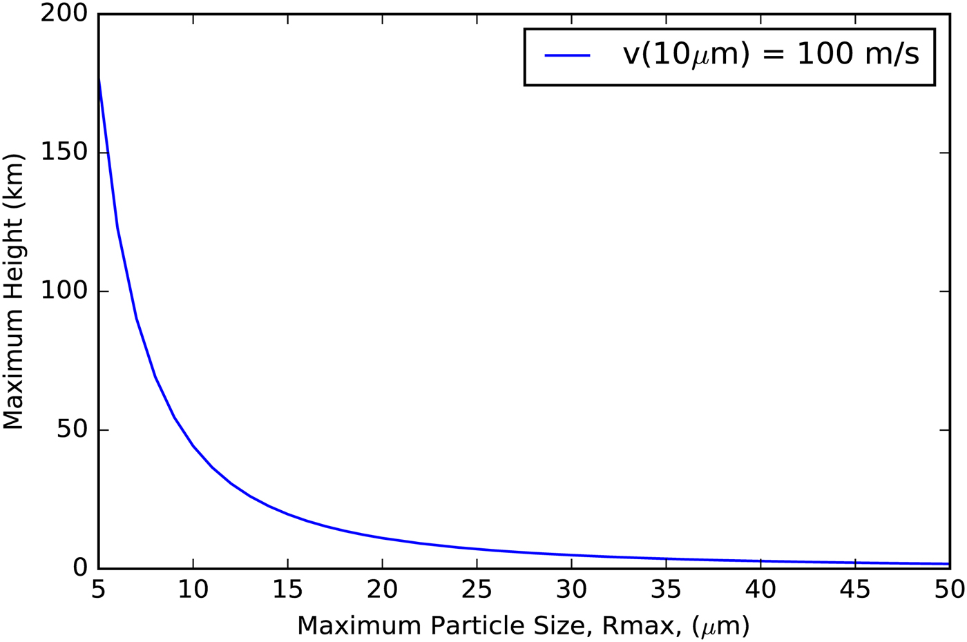
Fig. A6. Maximum height for a given maximum particle size, R max, based on simple kinematics.
We use Degruyter & Manga (Reference Degruyter and Manga2011) exit velocities to set the initial velocities of our particles as they leave the vent. Then particles are treated ballistically. In Fig. A6 we show the maximum height versus R max using our model's initial velocities and our v ~ 1/R velocity dependence. As described above, this dependence is limited by the gas velocities for smaller particles.
In addition, we say that as far as the data indicate larger collectors will collect more scaled simply to the area given a simple sweep up model, N(R) = n(R)×A×L where A is collector area, L is the path length through the plume and the statistical R max is when N(R) = 1.
Orbital variability
Plume variability with Enceladus orbital position as observed by the VIMS instrument and ISS instrument has been reported (Hurford, et al. Reference Hurford, Helfenstein, Hoppa, Greenberg and Bills2007; Hedman, et al. Reference Hedman, Gosmeyer, Nicholson, Sotin, Brown, Clark, Baines, Buratti and Showalter2013). Porco et al. (Reference Porco, Dones and Mitchell2017b) reported on the ISS observation that plume brightness changes by a factor of 0.5–2x with orbital phase and that this scales directly in mass production rate. In our model, if we double mass production rate indeed we double the sample mass. However, variations in orbit may be caused by more than just a change in production rate. There may also be variations in factors such as source geometry and configuration, particle size distribution, etc., with orbital position and this is an interesting area for future work. Possible decadal variability in plume activity has recently been suggested (Ingersoll & Ewald, Reference Ingersoll and Ewald2016), but is not considered in our plume modelling.


