


INTRODUCTION
In recent years, an increasing number of annually resolved radiocarbon (14C) records from tree rings have been published (e.g. Miyahara et al. Reference Miyahara, Masuda, Muraki, Kitagawa and Nakamura2006; Eastoe et al. Reference Eastoe, Tucek and Touchan2019; Fogtmann-Schulz et al. Reference Fogtmann-Schulz, Kudsk, Trant, Baittinger, Karoff, Olsen and Knudsen2019; Kudsk et al. Reference Kudsk, Philippsen, Baittinger, Fogtmann-Schulz, Knudsen, Karoff and Olsen2019). These high-precision datasets make it possible to investigate the occurrence of high-frequency cyclicities in solar activity, including the Schwabe (ca. 11 years) and Hale (ca. 22 years) cycles. The behavior of these cycles during Grand Solar Minima (GSMs) are of particular interest, as they have important bearings on our understanding of the solar dynamo. A GSM is a time interval characterized by lower solar magnetic activity than usual over a period of 30–160 years (Usoskin et al. Reference Usoskin, Gallet, Lopes, Kovaltsov and Hulot2016). The Maunder Minimum (1640–1720 CE, timing from Usoskin et al. Reference Usoskin, Gallet, Lopes, Kovaltsov and Hulot2016) is the only GSM which is covered by direct observations of sunspots. These observations show that the sunspots almost completely disappeared during the Maunder Minimum (Eddy Reference Eddy1976). For the period prior to the invention of the telescope in 1610 CE, the documentation of GSMs relies on indirect proxies of solar activity. Since 14C is formed in the atmosphere as a product of incoming cosmic rays, the production rate of 14C is correlated with the strength of the geomagnetic as well as the solar magnetic fields, which both shield the Earth from cosmic rays. The strength of the magnetic fields changes the cut-off rigidity necessary for cosmic rays to penetrate the atmosphere of the Earth. Since the geomagnetic field changes on millenial timescales (Dutta Reference Dutta2016), it can be regarded as stable on shorter timescales. Changes on a timescale of <100 years are therefore primarily due to changes in the solar magnetic field.
The 14C produced in the atmosphere is mixed with the stable carbon isotopes, 12C and 13C, and becomes part of the carbon cycle, where it eventually will be taken up in terrestrial archives, such as trees. The age of tree rings can be independently determined by dendrochronology, which makes 14C in tree rings an ideal proxy for solar activity. However, since the precision of the A accelerator M mass S spectrometry (AMS) measurements are of the same magnitude (2–3‰) as variations in atmospheric 14C associated with the Schwabe solar cycle (Stuiver and Braziunas Reference Stuiver and Braziunas1993; Baroni et al. Reference Baroni, Bard, Petit, Magand and Bourlès2011), it is difficult to resolve past changes in the solar cycle.
Several GSMs have been identified since the use of indirect proxies for solar magnetic activity began. Stuiver and Quay (Reference Stuiver and Quay1980) named the interval from 1282 to 1342 CE the Wolf Minimum, which was characterized by a maximum in 14C near 1340 CE, based on measurements of 14C in tree-ring samples that each spanned 10 years. Usoskin et al. (Reference Usoskin, Gallet, Lopes, Kovaltsov and Hulot2016) reconstructed the solar activity over the last nine thousand years based on 10Be and 14C records, and they identified the Wolf Minimum as spanning the years from 1270 to 1350 CE.
Hong et al. (Reference Hong, Park, Park, Sung, Lee, Park and Kim2013), and Eastoe et al. (Reference Eastoe, Tucek and Touchan2019) have published annually resolved 14C records based on tree rings covering the Wolf Minimum. Hong et al. (Reference Hong, Park, Park, Sung, Lee, Park and Kim2013) found peaks in a power spectrum of their annual dataset at 10.9 and 23.9 years corresponding to the Schwabe and Hale cycles, respectively. However, these periodicities were determined using the whole record spanning the years from 1250 to 1650 CE, and therefore it is unknown if these periodicities changed during the Wolf Minimum. The annual record of Eastoe et al. (Reference Eastoe, Tucek and Touchan2019) covered the years 998–1510 CE, and a spectral analysis of the whole record showed a peak corresponding to the Schwabe cycle at 10.4 years. The temporal evolution of the periodicities was investigated in a spectrogram, and in the time interval associated with the Wolf Minimum, there were indications of periodicities of 13.6 years and 26.4 years. More detailed information on the solar variability during the Wolf Minimum is needed to understand changes in the solar-cycle behavior during this GSM, and to resolve similarities and differences in solar activity among the different GSMs.
Eddy (Reference Eddy1976) noted that the Spörer (1390–1550 CE, Usoskin et al. Reference Usoskin, Gallet, Lopes, Kovaltsov and Hulot2016) and Maunder minima occurred at the time of the two most severe temperature decreases during the Little Ice Age (LIA), which was an unusually cold time period between ca. 1350 and 1850 CE (Brönnimann et al. Reference Brönnimann, Franke, Nussbaumer, Zumbühl, Steiner, Trachsel, Hegerl, Schurer, Worni, Malik, Flückiger and Raible2019), suggesting a relation between decreased solar activity and lower temperatures during the LIA. The exact definition of the LIA varies from study to study. Nagaya et al. (Reference Nagaya, Kitazawa, Miyake, Masuda, Muraki, Nakamura, Miyahara and Matsuzaki2012) suggested that the occurrence of the Wolf Minimum followed by the Spörer and Maunder minima could all have contributed to the lower than usual temperatures during the LIA, but the underlying mechanism and degree of causality remain uncertain. However, the timing of the Wolf Minimum does not coincide with that of the LIA. Instead, the beginning of the Wolf Minimum occurs at the end of the Medieval Climate Anomaly (950–1250 CE, Mann et al. Reference Mann, Zhang, Rutherford, Bradley, Hughes, Shindell, Ammann, Faluvegi and Ni2009), which could suggest the Wolf Minimum instead contributed to ending the Medieval Climate Anomaly. This coincidence between changes in climate and GSMs is intriguing and more knowledge about solar activity during this period could help provide a better understanding of the relationship between solar activity and the climate on Earth, and elucidate if the correlation between GSMs and climate changed over time.
In this paper, we present a new biennial 14C record based on measurements of tree rings from Danish oak covering the interval 1251–1378 CE. We compare the new results to the two above-mentioned annual records and perform frequency analysis to identify possible periodicities in the dataset. We also reconstruct the solar modulation potential across the Wolf Minimum, and compare it to the Spörer, Maunder, and Dalton minima.
METHOD
Eighteen archaeological samples of oak (Quercus sp.) found at Skjern Slot (Bjerringbro, Mid Jutland, Denmark, 56.45°N, 9.75°E, see Figure 1) were dated using dendrochronology (Bonde and Eriksen Reference Bonde and Eriksen2003). The 18 tree-ring sequences were averaged to form a site chronology (7044i001) ranging from 1239 to 1477 CE. This curve was crossdated with master chronologies from Jutland using the program DENDRO for Windows (Tyers Reference Tyers1999) following the methods outlined by Baillie and Pilcher (Reference Baillie and Pilcher1973). The master chronology best matching the Skjern Slot site chronology was that of Eastern Jutland (6m100001) with a t value of 11.11, thus validating the dendrochronological dates (Bonde and Eriksen Reference Bonde and Eriksen2003).

Figure 1 The red cross marks the location of the oak sample used for this study. (Please see electronic version for color figures.)
One of the 18 wood samples (70441029, G615, sample 2, hereafter referred to as SK2) with a tree-ring range of 1250–1425 CE was selected for AMS 14C dating. Individual ring widths of SK2 can be seen in Table S1 in the supplementary information. The tree-rings from 1250–1380 CE were separated into annual samples of early wood (EW) and late wood (LW) under a microscope using a surgeon scalpel. The LW samples from every second year were chosen for further analysis, as LW in oak has been shown to be a more robust recorder of past changes in the atmospheric radiocarbon levels than EW (Fogtmann-Schulz et al. Reference Fogtmann-Schulz, Østbø, Nielsen, Olsen, Karoff and Knudsen2017; Kudsk et al. Reference Kudsk, Olsen, Nielsen, Fogtmann-Schulz, Knudsen and Karoff2018), in part because EW may contain radiocarbon from the previous growth season (McDonald et al. Reference McDonald, Chivall, Miles and Bronk Ramsey2019).
The chosen LW samples were further pretreated to α-cellulose following the procedure described in Fogtmann-Schulz et al. (Reference Fogtmann-Schulz, Kudsk, Adolphi, Karoff, Knudsen, Loader, Muscheler, Trant, Østbø and Olsen2020), based on the method of Southon and Magana (Reference Southon and Magana2010). First, lignin was removed by treating with NaClO2 and HCl (2 times, 3 hr each, 70°C). After rinsing with 70°C milli-Q water, hemicelluloses were removed by treating with 17% NaOH (1 hr, room temperature). Lastly, after another rinse with 70°C milli-Q water, the samples were treated with 1 M HCl (30 min, 70°C) to remove any CO2 absorbed from the atmosphere during the step with the base treatment. The samples were then carefully rinsed with milli-Q water and freeze-dried.
The resulting α-cellulose fraction of the initial wood sample was in the range 32.2% to 48.8%, with most samples around 40%. According to Miller (Reference Miller1999), cellulose constitutes approximately 50% of wood substance in general, implying all samples experienced some loss of material. This was inevitable, especially during transfer of the sample from the glass vials used during pretreatment to the tube used for freeze-drying.
Next, the α-cellulose samples were prepared for measurement on an AMS system. The samples were first combusted to CO2 with CuO in sealed glass tubes. Then, the CO2 samples were purified and graphitized using the procedure of Olsen et al. (Reference Olsen, Tikhomirov, Grosen, Heinemeier and Klein2017). The radiocarbon fraction was then measured using a 1 MV HVEE Tandetron AMS system at Aarhus AMS Centre (AARAMS) at Aarhus University, Denmark (Olsen et al. Reference Olsen, Tikhomirov, Grosen, Heinemeier and Klein2017). To correct the measured 14C/12C ratios for isotopic fractionation, the 13C/12C ratio was measured online in the AMS system and subsequently normalized to a standard δ13C value of –25‰ Vienna Pee Dee Belemnite (Stuiver and Polach Reference Stuiver and Polach1977). The resulting radiocarbon ages are reported as conventional 14C dates in 14C years BP (Before Present = 1950 CE). Also reported are Δ14C values, which are calculated and age-corrected according to Stuiver and Polach (Reference Stuiver and Polach1977) and Jull et al. (Reference Jull, Panyushkina, Lange, Kukarskih, Myglan, Clark, Salzer, Burr and Leavitt2014).
The measured samples covered the timespan 1251–1378 CE, with two samples measured for every second year. To avoid using very narrow tree rings, uneven years were measured in the interval 1251–1367 CE, and even years were measured in the interval 1368–1378 CE. A total of 137 samples were measured from 65 individual LW tree rings.
The two individual measurements from the same year were combined by calculating a weighted mean for the samples that passed a reduced χ2 test. Seven years failed the χ2 test, and one extra sample was therefore measured for each of these years. The χ2 test was repeated for the 3 samples from the same year, but 6 of the 7 years still failed the test. A weighted mean was calculated for the one year that passed the test. For 5 of the remaining 6 years, the measurement with the greatest distance to the mean divided by the uncertainty was deemed an outlier. For the last year that failed the test, none of the individual measurements could clearly be deemed an outlier, and instead, the uncertainty was enhanced by multiplying with the square root of the χ2 value.
The resulting dataset was filtered with an infinite impulse-response low-pass filter with a stopband attenuation of 60 dB and a cut-off frequency of 1/5 yr–1 to reduce the year-to-year scatter and help identify long-term changes. The dataset was also filtered using a range of different bandpass filters, including (i) a filter with pass band frequencies of 1/40–1/16 yr–1 to study the Hale solar cycle, (ii) a filter with pass band frequencies corresponding to 1/16–1/7.1 yr–1 to study the Schwabe solar cycle, and a filter with pass band frequencies of 1/7.1–1/4.05 yr–1 to study other variabilities with higher frequencies. All the bandpass filters were sixth-order butterworth filters.
Furthermore, the dataset was analyzed with a Lomb-Scargle Fourier Transformation to identify the presence of significant periodicities. This was done using REDFIT (Schulz and Mudelsee Reference Schulz and Mudelsee2002), which calculated a power spectrum for the measured data and identified false-alarm levels based on comparison with red-noise data. The long-term variations in the dataset were removed prior to this analysis by subtracting a 34-yr moving mean.
In order to study variations of the solar magnetic field, we reconstructed the solar modulation function, Φ. First, the biennial data were linearly interpolated to a resolution of 0.1 yr. Next, the data were filtered with a lowpass filter with a cut-off frequency of 1/8 yr–1, and inserted into a carbon box model (Muscheler et al. Reference Muscheler, Beer, Kubik and Synal2005) to model changes in the 14C production rate. The IntCal20 data (Reimer et al. Reference Reimer, Austin, Bard, Bayliss, Blackwell, Bronk Ramsey, Butzin, Cheng, Edwards and Friedrich2020) were used in the interval from 10,000 BP to 1250 CE and from 1379 CE to 1800 CE to better constrain the box model in time intervals where we have no data. The modelled 14C production rate was combined with reconstructions of the geomagnetic field strength by Knudsen et al. (Reference Knudsen, Riisager, Donadini, Snowball, Muscheler, Korhonen and Pesonen2008) to estimate Φ (Masarik and Beer Reference Masarik and Beer1999). In order to estimate the uncertainty of Φ, the original Δ14C data were resampled 10,000 times using a normal distribution defined by the value and standard deviation of each Δ14C data point. The calculation of Φ was then repeated for each resampling. The final Φ estimate associated with each year was defined by the mean and standard deviation of these 10,000 values.
RESULTS
The average precision of the individual Δ14C measurements (Table S2 in the supplementary information) is ± 1.9‰, equivalent to ± 16 14C years. The combination of 2 or 3 measurements from the same year (Figure 2 and Table S2) yields a combined precision of ± 1.4‰, equivalent to ± 11 14C years.

Figure 2 The Δ14C record from this study is shown with blue circles. A lowpass filter with cut off frequency of 1/(5 yr) is shown for visual clarification with a light blue line. Data from Hong et al. (Reference Hong, Park, Park, Sung, Lee, Park and Kim2013) are shown with green triangles, and data from Eastoe et al. (Reference Eastoe, Tucek and Touchan2019) are shown with magenta triangles. The data from IntCal20 (Reimer et al. Reference Reimer, Austin, Bard, Bayliss, Blackwell, Bronk Ramsey, Butzin, Cheng, Edwards and Friedrich2020) are shown as a dark grey band including 1 σ error. The light grey box marks the interval of the Wolf Minimum (1270–1350 CE; Usoskin et al. Reference Usoskin, Gallet, Lopes, Kovaltsov and Hulot2016).
There is a general positive offset of 2.76 ± 0.23‰ between the new SK2 dataset from Danish oak and the IntCal20 curve (Reimer et al. Reference Reimer, Austin, Bard, Bayliss, Blackwell, Bronk Ramsey, Butzin, Cheng, Edwards and Friedrich2020) (Figure 2). A χ2 test of these two datasets failed, indicating that they are statistically different or the estimated errors are too small (χ2: 2.03 ≤ 1.31). The offset is largest for the early part of the record, whereas it becomes negligible after 1345 CE (Figure 2). When the samples were measured in the AMS, they were mixed in the different machine runs, i.e. they were not measured chronologically. Furthermore, there is nothing in the machine performance that suggests that these measurements were contaminated, the standard and background values were comparable to normal laboratory values.
Our SK2 dataset and the annual dataset of Hong et al. (Reference Hong, Park, Park, Sung, Lee, Park and Kim2013) have 65 years in common. Out of these 65 years, 22 years fail a χ2 test, implying they are statistically different and cannot be combined. The average difference in Δ14C values between these two datasets is 3.74 ± 0.51‰ (χ2: 3.60 ≤ 1.31). Hong et al. (Reference Hong, Park, Park, Sung, Lee, Park and Kim2013) noted an average offset of +40.0 14C years (i.e. older ages) compared to the IntCal04 data (Reimer et al. Reference Reimer, Baillie, Bard, Bayliss, Beck, Bertrand, Blackwell, Bronk Ramsey, Buck, Burr, Cutler, Damon, Edwards, Fairbanks, Friedrich, Guilderson, Hogg, Hughen, Kromer, McCormac, Manning, Reimer, Remmele, Southon, Stuiver, Talamo, Taylor, van der Plicht and Weyhenmeyer2004) for the period 1330 to 1430 CE. However, they did not provide an explanation for this offset. When comparing the Hong et al. (Reference Hong, Park, Park, Sung, Lee, Park and Kim2013) data to the IntCal20 data (Reimer et al. Reference Reimer, Austin, Bard, Bayliss, Blackwell, Bronk Ramsey, Butzin, Cheng, Edwards and Friedrich2020) for the time period 1330–1430 CE, the offset is +36 ± 3 14C years, equivalent to 4.52 ± 0.41‰. When subtracting the mean offset between the SK2 dataset and the Hong dataset, and repeating the χ2 test, 16 of the 65 years in common fail the test. We also subtracted a 35-year running mean from both datasets and repeated the χ2 test. This resulted in 14 failed years out of 65 years in common. The Hong dataset has an average precision of 32 14C years, i.e. more than three times higher than the average precision obtained in this study for the SK2 dataset when 2–3 samples are combined, and it also displays larger variability. To get a measure of the variability, we calculated the standard deviation of the difference between the sample values and a running mean (for 10 years) of the dataset. For the Hong dataset, this resulted in a variability of 5.4‰, whereas it is only 2.4‰ for the SK2 dataset. The larger variability associated with the Hong dataset, which possibly reflect local conditions and/or differences in wood cutting and measurement procedures, may explain the high number of years failing a χ2 test.
The annual dataset of Eastoe et al. (Reference Eastoe, Tucek and Touchan2019) has 59 years in common with our SK2 dataset. Out of these 59 years, 17 fail a χ2 test and are therefore statistically different. The average offset between these two datasets is 2.02 ± 0.29‰ (χ2: 2.69 ≤ 1.32). When this mean offset is subtracted from the data, 13 of the 59 years in common fail a χ2 test. If we subtract a 35-year running mean from both datasets, 11 of 59 years in common fail the test. This implies that our SK2 dataset is statistically different from the two existing annually resolved contemporaneous records based on χ2 tests, or that the associated errors are underestimated.
The variability of Δ14C over time is investigated with an amplitude spectrum (Figure 3A). This shows a peak corresponding to a period of 27 years above the 95% false-alarm level. There are furthermore two peaks above the 95% false-alarm level at 5.3 and 4.2 years. One peak additionally rises above the 90% false-alarm level at 9.1 years, but this is the only peak found near the 11-yr Schwabe cycle. The time evolution of these periodicities is visualized in a periodogram (Figure 3B). The periodicity around 9 years is present throughout most of the investigated time period, from ca. 1280 to 1340 CE, whereas the periodicity around 27 years is not significant between ca. 1290 and 1300 CE, indicating that this cyclicity weakened during part of the Wold f Minimum.
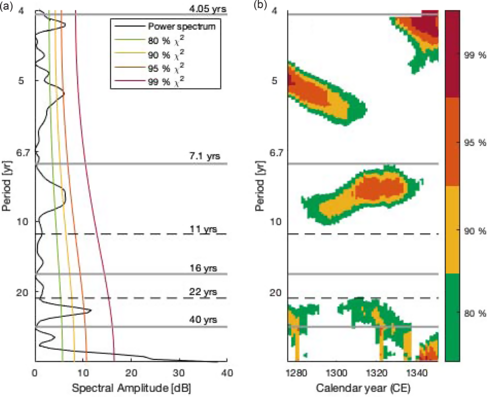
Figure 3 Amplitude spectrum (a) and time-resolved periodogram (b) of our data (black). The first and last 25 years are missing in the periodogram due to a window size of 50 years. A 34-year running mean filter has been subtracted from the data prior to these calculations. The black, dashed, horizontal lines mark periods of 11 and 22 years, respectively. The four grey horizontal lines mark the boundaries of the bandpass filters used in Figure 4 (4.05, 7.1, 16, and 40 years).
The variability of Δ14C is further investigated by applying different bandpass filters to the SK2 time series (Figure 4). In all the different bands, the amplitude is highest before and during the first half of the Wolf Minimum (1250–1310 CE). In the bandpass centered on the Hale cycle (16–40 years), the variability is greatly dampened from 1320 CE until the end of the time series (Figure 4C). A similar pattern is observed for the variability in the bandpass centered on the Schwabe cycle (7.1–16 years) (Figure 4B). A minimum amplitude is reached between 1345 and 1365 CE. The variability in the bandpass with periods of 4.05–7.1 years is also lowest after 1310 CE (Figure 4A). This high-frequency variability is of the same magnitude as the variability in the Schwabe- and Hale-centered bands during the Wolf Minimum.

Figure 4 Bandpass filtered Δ14C data. The different bands are confined by the periods written on the right side. The grey box marks the duration of the Wolf Minimum according to Usoskin et al. (Reference Usoskin, Gallet, Lopes, Kovaltsov and Hulot2016). The dashed black line marks the center year (1310 CE). The dashed red lines are plotted at ± 1.4‰, marking the average precision of these measurements.
The reconstructed solar modulation function, Φ, is shown in Figure 5. One cycle from 1250 to 1260 CE, characterized by a large magnitude, is followed by several cycles of reduced magnitude until 1360 CE. Thereafter, the magnitude of the cycles becomes larger again. The minima of the cycles before the Wolf Minimum (in 1250–1270 CE) are higher than the cycle minima during most of the Wolf Minimum (in 1270–1340 CE), whereas the cycle-minima values become larger towards the end of the Wolf Minimum (from 1340 CE onwards). A clear cyclicity with a duration between 8 and 10 years is evident in these data, particularly during the Wolf Minimum. The data were lowpass filtered with a cut-off frequency of 1/8 yr–1 prior to the calculation of Φ, which makes the ca. 9-yr periodicity stand out more clearly than in the original data.

Figure 5 Solar modulation function, Φ, reconstructed from the filtered radiocarbon record in blue. The grey band marks the standard deviation found by resampling the Δ14C values 10,000 times and calculating Φ for each resampling of the signal. Φ values based on 14C from Muscheler et al. (Reference Muscheler, Adolphi, Herbst and Nilsson2016) is shown in magenta. The light grey box mark the duration of the Wolf Minimum according to Usoskin et al. (Reference Usoskin, Gallet, Lopes, Kovaltsov and Hulot2016). On the right side, the mean values of Φ during the Dalton Minimum (DM), Maunder Minimum (MM), Spörer Minimum (SM), and Wolf Minimum (WM) from the Muscheler et al. (Reference Muscheler, Adolphi, Herbst and Nilsson2016) reconstruction is shown as well as the mean value of Φ during the Wolf Minimum based on the SK2 reconstruction.
DISCUSSION
The reconstruction of the solar modulation function, Φ, shows lowered solar activity during the Wolf Minimum. Vaquero et al. (Reference Vaquero, Gallego, Usoskin and Kovaltsov2011) suggested the Maunder Minimum was preceeded by two solar cycles of reduced activity, indicating a gradual transition into the Grand Minimum. Our reconstruction of Φ showed that the cycle from 1260 to 1270 CE, i.e. one cycle before the onset of the Wolf Minimum according to the definition of Usoskin et al. (Reference Usoskin, Gallet, Lopes, Kovaltsov and Hulot2016), was of similar amplitude as the following cycles that fall within the Wolf Minimum. This cycle could be a transitioning cycle, as suggested by Vaquero et al. (Reference Vaquero, Gallego, Usoskin and Kovaltsov2011).
The mean value of the reconstructed Φ during the Wolf Minimum (1270–1350 CE) is 255 ± 177 MeV. Muscheler et al. (Reference Muscheler, Adolphi, Herbst and Nilsson2016) reconstructed the solar modulation function based on the IntCal13 record for the northern (Reimer et al. Reference Hogg, Hua, Blackwell, Niu, Buck, Guilderson, Heaton, Palmer, Reimer, Reimer, Turney and Zimmerman2013) and southern hemispheres (Hogg et al. Reference Hogg, Hua, Blackwell, Niu, Buck, Guilderson, Heaton, Palmer, Reimer, Reimer, Turney and Zimmerman2013), as well as the annual radiocarbon record of Stuiver et al. (Reference Stuiver, Reimer and Braziunas1998) covering the last ca. 500 years. Their approach to calculating Φ was similar to the approach used in this paper, but the filter they applied was different. This reconstruction of Φ is shown in Figure 5. The mean value of Φ during the Wolf Minimum in the record of Muscheler et al. (Reference Muscheler, Adolphi, Herbst and Nilsson2016) was 269 ± 81 MeV, which is consistent with the result from this paper. We also calculated the mean value of Φ based on the reconstructed record presented in Muscheler et al. (Reference Muscheler, Adolphi, Herbst and Nilsson2016) during the Spörer Minimum (1390–1550 CE), Maunder Minimum (1640–1720 CE), and Dalton Minimum (1790–1820 CE) (Figure 5). The mean value during the Dalton Minimum was 520 ± 205 MeV, which is much higher than the mean value during the Wolf Minimum, revealing the Wolf Minimum to be considerably deeper than the Dalton Minimum. The mean values of Φ during the Spörer and Maunder minima were 211 ± 65 MeV and 195 ± 71 MeV, respectively, i.e. lower than the mean value during the Wolf Minimum. It is thus possible that that the Wolf Minimum was different from the Maunder Minimum in the sense that sunspots may have occurred regularly during the Wolf Minimum, as oppose to the Maunder Minimum that was characterized by extended periods with no sunspots.
In order to compare the Wolf Minimum to the three subsequent GSMs, we plotted our record of Φ together with the record of Φ from Muscheler et al. (Reference Muscheler, Adolphi, Herbst and Nilsson2016) across the Spörer, Maunder, and Dalton minima (Figure 6). The data were all lowpass filtered with a 1/16 yr–1 cut-off frequency to enable a better comparison of the overall shape of the different minima. The Dalton Minimum is clearly not as deep nor as long as the other minima. The Maunder Minimum is slightly deeper and wider than the Wolf Minimum, in part because the Wolf Minimum rises more steeply towards the end. The Spörer Minimum is of similar depth as the Maunder Minimum, but the duration of the Spörer Minimum is considerably longer. We note that the timespan officially associated with the Dalton Minimum (1790–1820 CE) seems misaligned with the Φ reconstruction of Muscheler et al., although this misalignmbet misalignment may partly relate to the filtering of the Φ reconstruction. For a comparison of the Δ14C values across the Wolf, Spörer and Maunder minima, see Figure S1 in the supplementary material
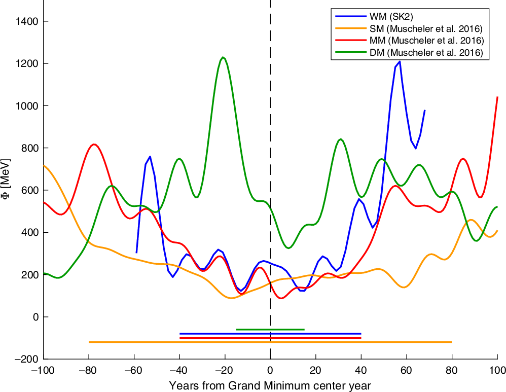
Figure 6 The solar modulation function, Φ, during the four most recent GSMs: The Dalton Minimum (green), Maunder Minimum (red), Spörer Minimum (orange), and Wolf Minimum (blue) plotted with respect to their center year (timing according to Usoskin et al. Reference Usoskin, Gallet, Lopes, Kovaltsov and Hulot2016 and Usoskin et al. Reference Usoskin2017), which is marked with a dashed, black, vertical line. The duration of the GSMs are marked with the horizontal lines in the bottom, the color corresponds to the color of the curve. The curves showing the Dalton, Maunder, and Spörer Minimum are the Φ reconstruction from Muscheler et al. (Reference Muscheler, Adolphi, Herbst and Nilsson2016) filtered with a lowpass filter with a cut-off frequency of 1/16 yr–1. The curve showing the Wolf Minimum is the Φ reconstruction from this paper (SK2) filtered by a lowpass filter with a cut-off frequency of 1/16 yr–1.
The variability in Δ14C in two bands centered on the Schwabe and the Hale cycle, respectively, is higher in the first 40 years of the Grand Minimum than in the last 40 years, implying that the Wolf Minimum was asymmetric with respect to the radiocarbon variability, as also observed for the Spörer Minimum (Fogtmann-Schulz et al. Reference Fogtmann-Schulz, Kudsk, Trant, Baittinger, Karoff, Olsen and Knudsen2019). This could indicate that the first half of a GSM has a slow decrease of amplitude until the overall minimum is reached, where after the amplitude rises more quickly to a non-GSM level. The variability in the band corresponding to periods of 4.05–7.1 years is of similar amplitude as the variability in the Schwabe band, and this makes it more difficult to detect the Schwabe cycle in the data. The exact cause of the 4–7-year variability is unknown, and we cannot rule out the possibility that it is strongly influenced by noise. However, Stuiver and Braziunas (Reference Stuiver and Braziunas1993) also found considerable variability in this period band (particularly around 5.1–6.4 years) in their Δ14C record from firs on the westcoast of the US. They suggested this variability was caused by changes in the ocean-atmosphere exchange associated with variations in upwelling related to the El Niño-Southern Oscillation (ENSO). Similarly, we propose that the 4–7-year variability in the SK2 dataset reflect changes in ENSO-related upwelling. It is also possible that changes in the ocean-atmosphere exchange related to the North Atlantic Oscillation contributed to the 4–7-year variability in the SK2 dataset. Olsen et al. (Reference Olsen, Anderson and Knudsen2012) found that the North Atlantic Oscillation (NAO) varied significantly with periodicities between 5 and 8 years in the past.
The power spectrum shows a peak at 27 years periodicity, being the only significant peak in the vicinity of the Hale cycle. Eastoe et al. (Reference Eastoe, Tucek and Touchan2019) also found a period of 26.4 years to be present in their annual 14C dataset around 1300–1330 CE, where after the period shortened between ca. 1330 and 1350 CE, and then returned to a period of 26.4 years from 1350 to 1375 CE. They also found some variability between ca. 1275 and 1325 CE with a period of ca. 13.6 years, but the amplitude was not high and the significance was not indicated.
Solanki et al. (Reference Solanki, Krivova, Schüssler and Fligge2002), Miyahara et al. (Reference Miyahara, Kitazawa and Nagaya2010), and Moriya et al. (Reference Moriya, Miyahara, Ohyama, Hakozaki, Takeyama, Sakurai and Tokanai2019) suggested that the Schwabe and Hale cycles lengthen during GSMs, which may also be the case in our record. However, the only significant peak close to the Schwabe cycle is the peak at 9.1 years, which may indicate the opposite, i.e. that the Schwabe cycle shortened during the GSM. Another possibility is that this is not the Schwabe cycle, in which case the amplitude of the Schwabe cycle must have been less than 1.4‰. The peak at 27 years may be the third harmonic of the 9.1-year periodicity, or it may be a lengthened Hale cycle.
CONCLUSION
Changes in atmospheric radiocarbon across the Wolf Minimum have been investigated with a new biennially resolved Δ14C record based on tree rings from Danish oak. Spectral analysis of the new Δ14C record revaled significant peaks at ~5.5 years, 9.1 years, and 27 years. This suggests that either the Schwabe cycle was shortened during the Wolf Minimum, or, alternatively, that the Schwabe cycle had an amplitude that was too small to be accurately identified during the Wolf Minimum. In contrast, the 27-year periodicity indicates that the Hale cycle was lengthened during the Wolf Minimum. Alternatively, 27-year periodicity could represent the third harmonic of the 9.1 years periodicity. The bandpass-filtered record showed dampened amplitudes of variability during the second half of the Wolf Minimum, and in the 30 years following the minimum in bands centrered on the Schwabe and Hale cycles, respectively. Variations in Δ14C with a period of 5.5 years most likely reflect changes in ocean-atmosphere exchange related to ENSO and the NAO.
A reconstruction of the solar modulation function showed a clear ca. 9-year period of variability, but also indicates that the interval characterized by low amplitudes began already in 1260 CE, implying that there was a gradual transition into the Wolf Minimum with one cycle of reduced activity preceeding the GSM.
A comparison of the solar modulation function during the Wolf Minimum with similar reconstructions covering the Spörer, Maunder, and Dalton minima showed that the Wolf Minimum resembles the Maunder Minimum with respect to duration and depth. The Wolf Minimum was deeper than the Dalton Minimum, but it was not quite as deep as the Maunder Minimum. However, the variability changes associated with the bandpass-filtered record resemble the variability during the Spörer Minimum more than the Maunder Minimum.
ACKNOWLEDGMENTS
We would like to acknowledge financial support from the Villum Foundation (VKR023114 and VKR010116). Funding for the Stellar Astrophysics Centre is provided by the Danish National Research Foundation (Grant Agreement DNRF106). We thank the staff at AARAMS for help with the laboratory work. We would also like to thank Raimund Muscheler for help with the carbon box model.
SUPPLEMENTARY MATERIAL
To view supplementary material for this article, please visit https://doi.org/10.1017/RDC.2020.126


