


Introduction
Rain fade refers to the absorption and scattering of a microwave signal by rain drops and it is a critical issue at frequencies above 10 GHz. Knowledge of the dynamics characteristics of rain fade is important for communication system designs since it determines the system availability and provides essential information for implementation of fade mitigation techniques. For that reason, it has received much attention during the last few decades [1–Reference Das and Maitra6]. Most of these studies were conducted on rain fade dynamics using data collected from temperate regions and various models were suggested. A well-known prediction model was proposed by the International Telecommunication Union-Radio (ITU-R) for earth to satellite links only. However, studies in [Reference Franklin, Fujisaki and Tateiba7–Reference Dao, Islam and Al-Khateeb10] have shown that the ITU-R fade slope model should be modified in order to suit tropical regions which are characterized by rainfall patterns that are different from temperate regions [Reference Mandeep and Allnutt2]. In addition, the modification should also consider the implementation of the model for terrestrial microwave links. This paper analyzes rain fade slope statistics obtained from rain attenuation data measured in Malaysia, and proposes an empirical model that can predict rain fade slope for point to point terrestrial microwave links.
This paper is organized as follows. “Fade slope models” section presents an overview of the known fade slope models available in the literature. Then, the fade slope data and the filtering process are described in the section “Fade slope data.” “Results and analysis” section compares the ITU-R fade slope model predictions with the measured results and then presents a new empirical model. Finally, “Conclusion” section concludes the paper.
Fade slope models
Fade slope is defined as the rate of change in rain attenuation with respect to time [Reference Dintelmann11] as illustrated in Fig. 1. Fade slope has been measured and analyzed in many experimental sites. Matricciani [Reference Matricciani12] studied the fade slope based on data collected from an 11.6 GHz satellite link in Italy. He found that the distribution of the fade slope for negative and positive rates is similar, and the threshold value does not affect the distribution. The same result was obtained by Dintelmann [Reference Dintelmann11] who also found that fade slope and fade duration are related.

Fig. 1. Graphical representation of the fade slope definition.
Sweeney and Bostian [Reference Sweeney and Bostian13] examined the dynamics of rain-induced fades on radio links by evaluating the rate at which the first Fresnel zone volume gets filled with rain. They have concluded that fade slope is very sensitive to changes in the rain rate. Nelson and Stutzman [Reference Nelson and Stutzman14] have studied rain fade dynamics using the data collected in Blacksburg-USA from the OLYMPUS satellite beacons at 12.5, 20, and 30 GHz. Their measured results have demonstrated that fade slope increases with frequency for a fixed occurrence level. They have also found that as the attenuation level increases, the occurrence of large fade slope increases. The same result is reported by Ruker [Reference Rücker15], who used data obtained from slant path propagation experiments carried out using the OLYMPUS satellite at 12.5, 20, and 30 GHz. He has concluded that the fade slope is frequency dependent, and occurs mostly in the high attenuation range. Furthermore, Miranda et al.[Reference De Miranda, Pontes and Da Silva Mello16] have analyzed fade slope data collected from three sites in Brazil. He has found that the distribution is almost symmetric. Van de Kamp [Reference Van de Kamp17, Reference Van de Kamp18] has derived a model in 1999 which was later adopted by the International Telecommunication Union Radio Communication Sector (ITU-R) as a global model in 2003. The ITU-R model [1] was tested using data collected at 12.5, 20, and 30 GHz from other locations in UK, France, Belgium, Italy, and USA. These results showed a good match with the shape of the fade slope distribution as well as its variation with attenuation levels. In the ITU-R model [1], the fade slope ξ was calculated for each sample from the following expression:
 $$\xi \lpar i \rpar = \displaystyle{{A\lpar i + 0.5\;{\rm \Delta }t\rpar -A\lpar i-0.5\;{\rm \Delta }t\rpar } \over {{\rm \Delta }t}}\;\lpar {\rm dB/s}\rpar \comma \;$$
where A is the rain attenuation, i is the sample number, and Δt is the length of the time interval. To calculate the conditional distribution of the fade slope, the following equation was proposed by the ITU-R [1]
 $$p\lpar {\xi \vert A} \rpar = \displaystyle{2 \over {\pi \sigma _\xi {\lpar {1 + {\lpar {\xi /\sigma_\xi } \rpar }^2} \rpar }^2}}\;$$
The only parameter that affects the distribution is the standard deviation, which can be approximated by
 $$\sigma _\xi = s\;F\lpar f_B\comma \;\;\Delta t\rpar A$$
where the coefficient s = 0.01, and the function F depends on the time interval length Δt and the 3 dB cut-off frequency of the low-pass filter fB. The function F can be expressed as:
 $$F\lpar f_B\comma \;{\rm \Delta }t\rpar = \sqrt {\displaystyle{{2\pi ^2} \over {{\lpar f_B^{{-}b} + {\lpar 2{\rm \Delta }t\rpar }^b\rpar }^{1/b}}}} $$
where b is a constant equal to 2.3. The bandwidth of the moving average filter is defined as:
 $$f_B = \displaystyle{{0.445} \over {t_a}}$$
where ta is the length of the moving average block.
Many researchers have found that the ITU-R model for fade slope perform reasonably well when compared with experimental data collected in temperate regions. For example, in England, Kastamonitis [Reference Kastamonitis, Gremont and Filip19] and Chambers [Reference Chambers, Callaghan and Otung20] compared the ITU-R model with measured data collected from satellite links at 20, 40, and 50 GHz. Both found that the ITU-R model is well fitted to the measured data. The same result was obtained by Garcia-Del-Pino in Spain at 50 GHz [Reference Garcia-del-Pino, Riera and Benarroch21]. In Finland, Salonen [Reference Salonen and Heikkinen22] compared the ITU-R model with the measured data from satellite link at a low elevation angle (12.7°). He also concluded that the prediction by the ITU-R model is close to their measured data. The same result was published in [Reference Singliar, Heder and Bito23] for terrestrial microwave link in Hungary. On the other hand, the same researchers in Hungary found that the ITU-R model should be modified to fit their data for other terrestrial microwave links [Reference Héder, Singliar, Katona and Bitó24]. They found that the ITU-R model does not fit to their measured data along terrestrial paths. Therefore, they have proposed a modified model which can be expressed as [Reference Héder, Singliar, Katona and Bitó24]:
 $$p\lpar {\xi \vert A} \rpar = \displaystyle{4 \over {\pi {{\sigma }^{\prime}}_\xi {\lpar {1 + {\lpar {\xi /{{\sigma }^{\prime}}_\xi } \rpar }^2} \rpar }^2}}\;$$
 The parameter  ${\sigma }^{\prime}_\xi $ was determined by the minimum root mean squared error. Moreover, Franklin and his team compared the ITU-R model with the measured data in Japan [Reference Mandeep5]. They found that the model does not fit the measured data and it needs to be improved. They modified the expression of the standard deviation which becomes:
 $$\sigma _\xi = \alpha \;F\lpar {\,f_{ 3{\kern 1pt} {\rm dB}}\comma \;{\rm \Delta }t} \rpar \;A\;\lpar {1 + \lambda \;{\rm ln}\lpar A\rpar } \rpar $$
where F(f 3dB, Δt) is as mentioned in (4), and the factor λ is equal to 0.32. From their measurement, the fade slope distribution behavior was found to be different from the one proposed by the ITU-R. They observed that the shape of the fade slope distribution had a return point between 7 and 8 dB in all stations and it is independent of the sampling period.
Fade slope data
The measured data considered in this paper was collected from three experimental mini links installed by Ericsson at the University of Technology Malaysia in Johor campus (1.5333°N, 103.6667°). The frequencies used by these mini-links are 15, 23, and 38 GHz with a hop length of 300 m. The main features of these mini-links are summarized in Table 1. The collected data were directly obtained from the measurement of the automatic gain control (AGC) voltage level at the receiver side by using a data acquisition card of type PCL-718. Then the data were converted into the received power level using the calibration chart supplied by the manufacturer. The data were collected every second during raining events. If it is not raining, the average value of the data is stored every minute. The data were measured for a period of 16 months with the availability of the links shown in Table 1. The rain attenuation data were extracted from the received signal level using Matlab. A real-time rain gage was also installed and synchronized in time with the mini-link data acquisition system.
Table 1. Mini link specification details

During rainfall, the received signals have two components: rain attenuation and scintillation. To study the rain fade, fast fluctuation due to scintillation is filtered out before analysis. Based on [Reference Matricciani and Riva25], the rain attenuation time series can be obtained by filtering the measured data time series through a Butterworth low-pass filter with a cutoff frequency of about 0.025 Hz. In [Reference Van de Kamp18] and [Reference Baxter, Upton and Eden26–Reference Van de Kamp and Castanet28], low-pass filtering was used by applying moving average windows of lengths varying from 10 s to 2 min. In this study, the scintillation is removed by using a 20 s moving average filter which corresponds to a low-pass filter with a cut-off frequency of 0.022 Hz. The output can be expressed as
 $$A\lpar t\rpar = \displaystyle{1 \over {1 + t_a}}\;\mathop \sum \limits_{t-t_a}^t A\lpar t_i\rpar \;$$
where ta = 20 s and t is time in seconds.
Another issue of concern is the accuracy of the rain attenuation data obtained from the measurement system. This can be resolved by computing the measurement uncertainty of the system following the GUM recommendations [29]. For this purpose, a number of sources of uncertainty are considered based on their significant contribution. This includes uncertainties due to calibration, resolution, and repeatability which are associated with the data acquisition card PCL-718. The accuracy and the resolution of the PCL-718 card are provided in its specification sheet, while the repeatability errors was estimated using 10 sampled data measured during non-raining events. Another source of uncertainty is produced from the conversion of AGC voltage into the received power level. Rafiqul [Reference Islam30] had demonstrated that the AGC conversion will introduce a maximum error of 2% when computing the rain attenuation. Considering all these factors and taking into account the averaging of the AGC level, the combined standard uncertainty was determined for five attenuation values with 95% confidence and the results are shown in Table 2. It is clear that the AGC conversion significantly contributes to measurement uncertainty and it is the dominant factor because the maximum error is about 2% for attenuation values higher than 3 dB. Since this study is dealing with rain attenuation data with values higher than 0.5 dB, in worst case the maximum error will not exceed 5% and this can be tolerated.
Table 2. Combined standard uncertainty with 95% confidence for the three links at various attenuation values

The fade slope statistics are analyzed by calculating the conditional probability density function (CPDF). For each sample i the fade slope ξ(i) is calculated from (1). The conditional distributions at the attenuation level A (in dB) is calculated based on all the attenuation values A(t) that satisfy the following inequality:
 $$A-0.5 \lt A\lpar t\rpar \le A + 0.5$$
where A = 1, 2, 3, 4,… dB. For example, the 1 dB distribution is obtained considering all the slopes calculated using (1) for an attenuation A(t) between 0.5 and 1.5 dB [Reference Garcia-del-Pino, Riera and Benarroch21, Reference Salonen and Heikkinen22]. The distribution characteristics and its behavior are discussed in the next section.
Results and analysis
The fade slope of the measured data was calculated for each attenuation level from (1). These data are used to compute the CPDF distribution behavior which is compared with the predictions from the ITU-R model. A detailed description of this comparison is presented in the next section. Then, a new empirical model based on the data from the 23 GHz link is proposed in the section “Proposed model for fade slope prediction.” Finally in the last section, the model is validated using the data from the 15 and 38 GHz links. This validation is made possible since earlier studies in [Reference Zyoud, Dao, Islam, Chebil, Al-Khateeb and Abd Rahman9, Reference Van de Kamp18, Reference Garcia-del-Pino, Riera and Benarroch21, Reference Islam, Chebil, Khalifa, Khan, Dao and Zyoud31] have shown that the fade slope distribution is independent of frequency.
Comparison of fade slope data with the ITU-R model
The CPDFs of the measured fade slope data at 23 GHz were compared with the ITU-R model for different attenuation levels 1, 3, 5, 8, 10, and 15 dB as illustrated in Fig. 2. The results show that the ITU-R model is only close to the measured data at 1 dB level, but far away for all other attenuation levels. This problem is mainly due to the selected value for the standard deviation which affects the distribution. It is found that the standard deviation values used by the ITU-R curves are generally higher than those obtained from the measured data. Similar behavior is also observed for the other two links. In order to predict the fade slope probability density functions for terrestrial microwave links, this study suggests improving the ITU-R model by modifying the expression of its distribution and its standard deviation. This will be discussed further in the next section.
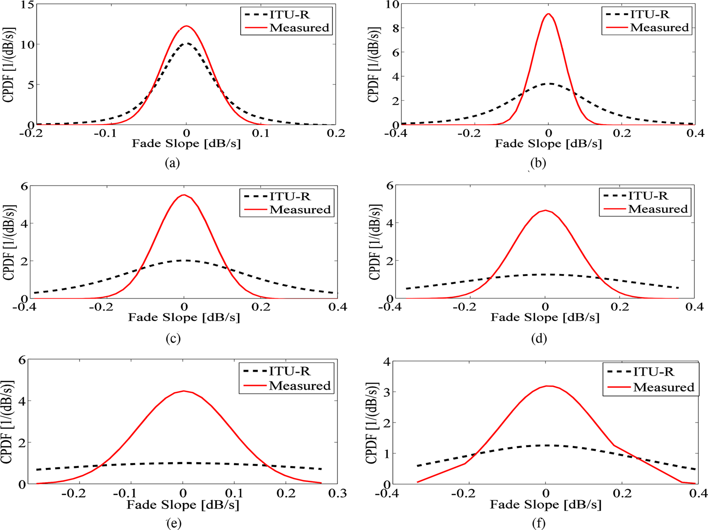
Fig. 2. The CPDF of fade slope for measured data with the ITU-R predictions at 23 GHz for attenuation levels at: (a) 1 dB; (b) 3 dB; (c) 5 dB; (d) 8 dB; (e) 10 dB; and (f) 15 dB.
Proposed model for fade slope prediction
The conditional distribution functions of the fade slope for the attenuation levels 1, 3, 5, 8, 10, and 15 dB at 23 GHz are plotted in one graph in Fig. 3. The following observations are noted. First, all the fade slope distributions here are symmetric around 0 dB/s which confirm the finding of other researchers [Reference Nelson and Stutzman14, Reference De Miranda, Pontes and Da Silva Mello16–Reference Kastamonitis, Gremont and Filip19, Reference Garcia-del-Pino, Riera and Benarroch21]. Second, all the CPDFs follow normal distribution with zero average. Third, the distribution becomes broader when the attenuation level increases. Finally, the magnitude of the fade slope increases with the attenuation level, however the amount of data decreases.

Fig. 3. The CPDF of the fade slopes for different attenuation levels measured at 23 GHz in Malaysia.
To prove that the fade slope distribution follows the normal distribution, the T-test is used. Two hypotheses are considered for the T-test. The first one is the null hypothesis (H = 0) which considers the measured data follow a normal distribution with mean μ = 0. While the second one is the alternative hypothesis (H = 1) which considers measured data follow a normal distribution with mean μ ≠ 0. The T-test statistics that is used is described by [Reference DeCoursey32]
 $$t = \displaystyle{{\bar{x}-\mu } \over {\sigma /\sqrt n }}$$
where  $\overline x $, σ are the mean and standard deviation of the tested data. The size of the data is represented by n. The results of the test are summarized in Table 3 and it shows that the T-test succeeds for all attenuation levels at 23 GHz considering a significance level of 0.05. This means that the null hypothesis is accepted with a confidence level of 95%.
Table 3. T-test results for the data measured from the 23 GHz link

Since the data follow the normal distribution with zero mean for all attenuation levels so the probability distribution can be expressed as [Reference DeCoursey32, Reference De Miranda, Quesnel and Da Silva Mello33]
 $$p\lpar \xi \vert A\rpar = \displaystyle{1 \over {\sigma _\xi \sqrt {2\pi } }}\exp \left({0.5{\left({\displaystyle{{\xi -\mu } \over {\sigma_\xi }}} \right)}^2} \right)$$
The only parameter that affects the distribution in this equation is the standard deviation. To derive an expression for this parameter, the standard deviation is plotted in Fig. 4 as a function of the attenuation levels measured at 23 GHz. By using Matlab fitting tools, the best fit can be described by
 $$\sigma _\xi = 0.00012A^3-0.003A^2 + 0.027A-0.0016\;$$
Fig. 4. Comparison between the estimated and measured standard deviation as a function of attenuation levels at 23 GHz.
The good fit is verified from the curve of (12) in Fig. 4. Since the mean is equal to zero, so (11) can be rewritten as
 $$p\lpar {\xi \vert A} \rpar = \displaystyle{1 \over {\sigma _\xi \sqrt {2\pi } }}\exp \left({0.5{\left({\displaystyle{\xi \over {\sigma_\xi }}} \right)}^2} \right)$$
From the above analysis, equations (12) and (13) can be used as a new model for predicting the fade slope distribution. To test its performance, Fig. 5 shows the plots of both the CPDF of the fade slopes from the new model and from the measured data for various attenuation levels at 23 GHz. It is clear that the new model fits well the measured data at all attenuation levels except at 1 and 3 dB. However, by comparing the results in Figs 2(b) and 5(c), the predicted distribution by the new model is better than that of the ITU-R for the 3 dB level. It can be concluded that the new model can perform better than the ITU-R model for any attenuation level above 2 dB. The validity of the proposed model is presented in the next section.

Fig. 5. Comparison between the predicted CPDF of fade slopes from the proposed model and the measured data at 23 GHz for attenuation levels at (a) 1 dB; (b) 2 dB; (c) 3 dB; (d) 5 dB; (e) 8 dB; and (f) 15 dB.
Validation of the new model
To verify the proposed empirical model, the fade slope data measured from the 15 and 38 GHz radio links are used. The CPDF of fade slopes from the proposed model and the measured data at 38 GHz are shown in Fig. 6. Similar outcome was observed if the measured data at 15 GHz were used. The results show that the proposed model fits very well the data for any attenuation levels higher than 2 dB for both frequencies. However, this observation is not sufficient since we should take into considerations the uncertainty in the measured data. For this reason, the new model is validated using the chi-square goodness-of-fit test which is a well-known method. This test determines how well the proposed distribution fits the measured distribution using hypothesis testing for a given significance level which is commonly taken as 0.05 [Reference DeCoursey32]. The test is applied to the fade slope data measured from the 15, 23, and 38 GHz radio links. The first step in this method is to define the null hypothesis: H0, and the alternative hypothesis: Ha.
H0: There is no significant difference between the measured and the expected values.
Ha: There is a significant difference between the measured and the expected values.
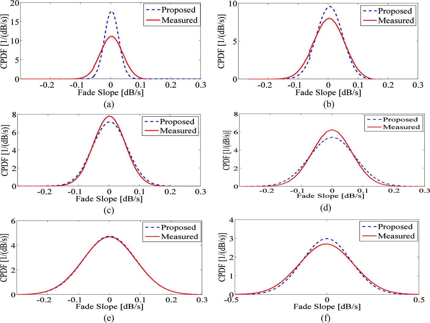
Fig. 6. The CPDF of fade slopes from the proposed model and the measured data at 38 GHz for attenuation levels of (a) 1 dB; (b) 2 dB; (c) 3 dB; (d) 5 dB; (e) 8 dB; and (f) 15 dB.
In the next step, the chi-square test is determined using [Reference DeCoursey32]
 $$\chi _{comp}^2 = \mathop \sum \limits_{i = 1}^N \displaystyle{{{\lpar O_i-E_i\rpar }^2} \over {E_i}}$$
where  $\chi _{comp}^2 $ represents the computed χ 2 value, Oi is the observed or the measured sample, Ei is the expected sample, and N is the number of samples. In this case, the number of degree of freedom (df) is equal to N − 1. The computed values for
  $\chi _{comp}^2 $ and df are shown in Table 4 for the three types of measured data. Then, the theoretical χ 2 value,
 $\chi _{th}^2 $, is determined for a degree of freedom df and a significance level of 0.05 using Matlab and the results are also presented in Table 4. It is noted that for attenuation levels higher or equal to 2 dB, the values of
  $\chi _{comp}^2 $ are found less than those of
  $\chi _{th}^2 $ for all three links. Therefore, the null hypothesis H0 is accepted and it can be concluded that there is no significant difference between the predicted and measured values for the three cases. This means the proposed model is a good fit for attenuation levels larger than 2 dB for the three frequencies. However, the model did not produce a good fit for an attenuation level of 1 dB since
  $\chi _{comp}^2 {\rm \gt }\chi _{th}^2 $.
Table 4. The computed  $\lpar \chi _{comp}^2 \rpar $ and the theoretical
  $\lpar \chi _{th}^2 \rpar $χ 2 values for a significance level of 0.05 are shown along the degree of freedom (df) for the three experimental links

Conclusion
This paper proposes a new empirical model for the prediction of rain fade slope for point to point terrestrial microwave links in tropical regions such as Malaysia. The study is based on measured rain fade slope data which were obtained from three terrestrial microwave links installed in Malaysia and operating at 15, 23, and 38 GHz. Unlike the ITU-R earth-to-satellite rain fade slope model for earth-to-satellite links, it is found that the measured fade slope distribution at 23 GHz is better approximated by normal distribution with mean equals to zero. A new prediction model is derived based on analysis of the measured data at 23 GHz. The proposed model is tested with the measured fade slope data at 15 and 38 GHz and it is found in close agreement with almost all attenuation levels. Furthermore, the model is validated using the chi-square goodness-of-fit test. The proposed model will be a useful tool in designing rain fade mitigation techniques for terrestrial links in tropical regions.
Acknowledgement
This work is partially funded by International Islamic University Malaysia (IIUM) Publication Research Initiative Grant Scheme P-RIGS18-003-0003. The authors are also grateful to the Wireless Communication Centre at the University of Technology Malaysia for supporting this research by providing the data.
 Jalel Chebil received his bachelor and master degrees in electrical engineering from the University of Wisconsin Madison, USA in 1987 and 1990, respectively. He also completed his Ph.D. in electrical engineering from the University of Technology Malaysia in 1998. He is currently working in the University of Sousse, Tunisia. He has authored and co-authored many research papers in international journals and conferences. His main research interests include radio wave propagation, wireless channel modeling, antennas, and digital signal processing.
 Md. Rafiqul Islam (M’01–SM’18) received his B.Sc. degree in electrical and electronic engineering from the Bangladesh University of Engineering and Technology, Dhaka, Bangladesh, in 1987, and his M.Sc. and Ph.D. degrees in electrical engineering from the University of Technology Malaysia in 1996 and 2000, respectively. He is currently a Professor with the Department of Electrical and Computer Engineering, International Islamic University Malaysia, Kuala Lumpur, Malaysia. He has authored or co-authored more than 300 research papers in international journals and conferences. His research interests include wireless channel modeling, RF propagation measurement, and modeling. Prof. Islam is a Life Fellow of Institute of Engineers, Bangladesh and a member of the IET.
 Al-Hareth Zyoud (M’18) received his bachelor degree in electrical engineering from Palestine Polytechnic University in 2006, his master and Ph.D. degrees in communication engineering from International Islamic University Malaysia in 2011 and 2017, respectively. He has authored or co-authored many research papers in international journals and conferences. His current research interests include RF modeling and simulation, 5G radio resource management, and rain attenuation analysis.
 Mohamed Hadi Habaebi (M’99–SM’16) received his first degree from Civil Aviation and Meteorology High Institute, Esbeiaa, Libya, in 1991, his M.Sc. degree in electrical engineering from Universiti Teknologi Malaysia in 1994, and his Ph.D. degree in computer and communication systems engineering from Universiti Putra Malaysia in 2001. He is currently the Head of the Department and a professor at the Electrical and Computer Engineering, International Islamic University Malaysia, Kuala Lumpur, Malaysia. He is the founding member of IoT and wireless Communication Protocols Laboratory with the same department. He has supervised many Ph.D. and M.Sc. students, authored or co-authored more than 200 articles and papers, and sits on the editorial board of many international journals. He is actively reviewing and publishing in computer communications, wireless sensor and actuator networks, cognitive radio, small antenna system & radio propagation, and wireless communications & network performance evaluation.
 Hassan Dao received his bachelor degree in computer engineering in 2002 from Sripatum University, Thailand. He also received his M.S. and Ph.D. from the International Islamic University Malaysia in 2007 and 2013, respectively. He is currently a lecturer at the ECE Department, Faculty of Engineering, Princess of Naradhiwas University, Thailand. He has published several papers in international journals and conferences. His research interests include signal processing communication, image processing, radio link design, RF propagation measurement, and wireless communication.


