


NOMENCLATURE
- D
-
non-swirl jet diameter, mm
- Dh
-
hub internal diameter, mm
- D oh
-
hub outer diameter, mm
- D os
-
swirl outer diameter, mm
- Ds
-
swirl diameter, mm
- L
-
length of the pipe, mm
- L/D
-
length to diameter of the pipe
- M
-
mach number
- n
-
number of vanes
- P0
-
settling chamber pressure, Pa
- Pa
-
ambient pressure, Pa
- Pe
-
jet exit pressure, Pa
- Pt
-
total or pitot pressure
- S
-
swirl number
- tb
-
blade thickness, mm
- th
-
hub thickness, mm
- w
-
width of the swirler, mm
- ϑ
-
vane angles, degrees
- BSAN
-
Broadband Shock-Associated noise
- EA
-
Emission Angle
- NPR
-
Nozzle Pressure Ratio
- OASPL
-
Overall Sound Pressure Level
- SCV
-
Swirler – Curved Vane
- SFV
-
Swirler – Flat Vane
- SPL
-
Sound Pressure Level
Abbreviations
1.0 INTRODUCTION
The applications of swirling flows are widely recognised in many research areas over a broad range of Mach numbers from subsonic to supersonic conditions. The swirling flows usually enhance the mixing and the spreading rate(Reference Park and Shin1,Reference Abdelhafez and Gupta2) compared to non-swirl or free jets. At certain high swirl numbers, the core expands and causes the generation of a vortex breakdown. This enhances the mixing between the fuel and the oxidizer and acts as a flame holder in the combustion chamber. Also, the addition of swirling flows causes a reduction of noise levels(Reference Schwartz3,Reference Schwartz4) . Apart from these applications, swirling flows are used in confined configurations such as combustion, cyclone separators and pipe flow systems, systems for transport of sand, gravel(Reference Elsner and Kurzak5–Reference Ariyaratne9) and so on. The advantages of swirl are heat transfer enhancement, mixing enhancement, reduction of pressure losses in bends, fittings and so on. The importance of swirl can be understood from research findings that the augmentation of heat transfer is a strong function of the swirl number and less dependent on Reynolds number(Reference Dhir10).
Thus, the existing literature on confined swirl systems mainly focuses on flow and mixing characteristics. There is not much research on the noise effects of confined swirl systems. Hence, the present experimental work is devoted to the study of the noise and flow field characteristics of co-axial swirl pipes over a range of Mach numbers.
1.1 Swirl number and flow field characteristics of co-axial swirl pipe flows
The swirl number is used to quantify the amount of swirl is added into the given flow system. It is the ratio of the axial flux of swirl momentum (Gθ) to the product of axial flux of axial momentum (Gx), and the equivalent nozzle radius (R), as shown in Equation (1):
 $$\begin{equation}
S = \frac{{{G_\theta }}}{{{G_x}R}}
\end{equation}$$
$$\begin{equation}
S = \frac{{{G_\theta }}}{{{G_x}R}}
\end{equation}$$
However, for fixed vane angle configurations (flat or curved), the swirl number equation can be written(Reference Alekseenko, Dulin, Kozorezov and Markovich11) as,
 $$\begin{equation}
S = \frac{2}{3}\left( {\frac{{1 - {{\left( {{D_h}/{D_s}} \right)}^3}}}{{1 - {{\left( {{D_h}/{D_s}} \right)}^2}}}} \right){\rm{tan}}\theta ,
\end{equation}$$
$$\begin{equation}
S = \frac{2}{3}\left( {\frac{{1 - {{\left( {{D_h}/{D_s}} \right)}^3}}}{{1 - {{\left( {{D_h}/{D_s}} \right)}^2}}}} \right){\rm{tan}}\theta ,
\end{equation}$$
where, Dh and Ds are hub and swirler diameters in mm. θ is the vane angle in degrees.
In the present work, at the downstream of the swirler, a confined pipe system is attached. However, there are no standard methods to quantify the swirl number in such flow conditions. Further, the Equation (2) is used for the present work in order to define the swirl numbers with respect to the vane angles.
The swirl can be generated by means of fixed or movable vanes, tangential injections, rotating pipes, twisted pipes, propeller types, and so on. The swirl number can be weak or high and strongly depends on the vane angle.
Figure 1 shows the flow characteristics of co-axial swirl pipe jets. The inner and outer (annular) streams are separated by the inner pipe wall. In the annular passage, flow enters through curved blades to generate a swirl, while the inner (primary jet) pipe flow evolves as a free pipe jet. The co-axial swirl pipe jet consists of a primary potential core, an annular secondary potential core and inner and outer mixing layers. The region where the primary and secondary shear layers develop and the secondary core disappears is called the initial merging zone. The primary core still exists and the mixing and merging of the primary and secondary shear layers occur in the intermediate zone. In the fully merged region, the primary core disappears, and the region is entirely dominated by eddies.

Figure 1. Flow structures of co-axial swirl pipe.
The confined co-annular swirl jet with swirl in annular passage was studied by Dinesh et al(Reference Dinesh, Savill, Jenkins and Kirkpatrick12), who observed that the jet spreads more radially with increase in swirl velocity, due to the presence of the centrifugal force. They also observed that an increase in swirl leads to a decrease in the centre line velocity. Similarly Ribeirio and Whitelaw(Reference Ribeiro and Whitelaw13) conducted experiments on co-axial jets with and without swirl. It was observed that, when the swirl is introduced in the outer stream, the near field becomes complicated and swirling flows show higher spread rates.
However, at supersonic conditions, the shocks/expansion waves appear in the both primary and secondary cores. These two core shocks interact with each other at the exit of the pipes, and the extent of interaction depends on the swirl number or vane angle.
1.2 Acoustic characteristics
The principal noise sources are turbulent mixing noise (at subsonic and supersonic conditions), transonic tones (at transonic Mach numbers), Broadband Shock-Associated Noise (BSAN), and screech tones (at supersonic imperfectly expanded conditions).
The turbulent mixing noise is caused by the mixing of the pipe jet fluid with the surrounding ambient fluid. The turbulent mixing noise originates from both the large- and fine-scale turbulent structures. When the large-scale turbulent eddies are convected at supersonic speeds with respect to the surrounding ambient fluid, Mach waves are generated(Reference Tam, Golebiowski and Seiner14), which are dominant noise sources in supersonic conditions. The transonic tones are observed at low Nozzle Pressure Ratios (NPRs) (1.6 ≤ NPR ≤ 1.9) due to the presence of shock waves in the diverging portion of CD nozzle(Reference Zaman, Dahl, Bencic and Loh15) and also in other jet configurations(Reference Jothi and Srinivasan16). The BSAN emerges from the interactions of the downstream convecting large-scale structures with the shock cells. BSAN is a strong function of Mach number and it occurs usually at frequencies higher than the screech tone. The instability waves originating at the nozzle lip interact with the quasi-periodic shock cell structures to generate acoustic waves. The acoustic waves propagate upstream and hit the nozzle lip, triggering the next sequence of instability waves, thus completing an acoustic feedback loop. This feedback loop generates screech tones which are discrete tones with high amplitudes. In some cases, screech tone appears with its harmonic tones, and it is usually dominant at upstream angles.
In the 1970s, Schwartz(Reference Schwartz3,Reference Schwartz4) proposed that noise intensity can be reduced by using vanes. Later, Lu et al(Reference Lu, Ramsay and Miller17) developed an experimental work to study the noise of the swirling exhaust flows. The swirling jet noise was higher than the non-swirling jets, except at angles less than 40° from the jet axis. Yu et al(Reference Yu and Chen18) studied tangential injection swirling flows and observed that swirl flow reduce the shock cell spacing compared to non-swirling flows. A high subsonic co-axial jet of Mach 0.9 was simulated by Andersson et al(Reference Andersson, Eriksson and Davidson19), who observed the high levels of turbulent kinetic energy in the secondary core outer shear layers, which lead to an increase in the sound pressure levels. Co-axial jet noise source distribution experiments were conducted by Rostamimonjezi(Reference Rostamimonjezi20). The results showed that the addition of the secondary flow reduces the convective velocity of the eddies in the primary layers, which helps to attenuate the Mach waves. The present work studies the noise and flow characteristics of confined co-axial pipe with swirl in the annular passage (secondary core) and free jet at the centre of the jets (primary core). To the knowledge of the authors, such a configuration has not been studied in the literature, and has potential applications in combustors and mixing systems.
2.0 EXPERIMENTAL METHODS AND PROCEDURES
This section briefly explains the experimental set-up and the procedure of the experiments carried out.
2.1. Anechoic chamber and instrumentation
Figure 2 shows the layout of the anechoic jet test facility at Thermodynamics and Combustion Engineering Laboratory, Department of Mechanical Engineering, IIT Madras. The air is compressed using a150HP, Khosla reciprocating compressor located outside the laboratory. The compressed air is dried and filtered before entering the settling chamber in which wire meshes are installed to remove any flow disturbances.

Figure 2. Layout of Anechoic chamber with Data acquisition system (Dimensions are in m).
The pressure is continuously monitored by a bourdon tube pressure gauge and a piezo- resistive pressure transducer inside the settling chamber. The acoustic far field measurements are carried out using a ¼-inch condenser microphone (PCB 377A01) with a sensitivity of 4mV/Pa. A Piezo-resistive pressure transducer (Endevco Model 8510C-100) was connected to a pitot probe to measure the total pressure along the jet center line. A high-speed digital camera (Mikrotron MC1302) was used for recording the schlieren images. The data were acquired using National Instruments data acquisition board NI-PCI-6143, which was controlled by Labview 2014.
2.2. Test models and methods of measurements
Figure 3 shows the schematic of co-axial swirler used in the present experimental work. The swirl jet inner (Ds ) and outer (Dos ) diameters are 14mm and 16mm, respectively. The internal hub (Dh ) and width (w) of the swirler are 6mm each. The curved blade thickness (tb ) and hub thickness (th) are 1mm each, and the number of blades (n) is 6.

Figure 3. Co-axial swirl jet model and blade position (only one blade shown here).
The notation is used “Swirler – Curve Vane” (SCV) followed by curved vane angle. That is, SCV20 denotes co-axial curved vane pipe swirler at 20° vane angle. The non-swirl pipe jet has a diameter (D) of 12mm, in order to maintain almost equal momentum for swirl and non-swirl pipe jets. The pipe lengths for the present experiments are L=0.5D and 2D from the exit of the swirler (Fig. 1). The swirl number is calculated using the Equation (2), and listed in Table 1. The pipe jets are manufactured using Eden 350V Rapid Prototyping Machine at Department of Engineering Design, IIT Madras and the material used was photopolymer resin.
Table 1 Swirl Numbers for various curved vane swirlers

SCV - Swirler Curve Vane, SFV - Swirler Flat Vane
* Although there is no tangential velocity, vortices are shed from the trailing edge of vanes
The acoustic measurements are carried out in the acoustic far field region of 34D and the microphone measurement angles (Emission Angle (EA)) span across an upstream angle of 135° to a downstream angle of 35° with an increment of 5°.
2.3. Validation
For the purposes of validation, the transonic fundamental frequency is compared with data available in the literature, as shown in Table 2. The frequencies are not exactly the same, but close to each other. The variations in the frequencies are due to different jet configurations and flow conditions. At supersonic conditions, the screech frequency for the non-swirl pipe jet (L/D=2) is validated with the results of Dhamanekar and Srinivasan(Reference Dhamanekar and Srinivasan21) and the screech frequency formula given by Gao and Li(Reference Gao and Li22). The comparisons are shown in Fig. 4. The present results show only helical modes, in line with results of Dhamanekar and Srinivasan(Reference Dhamanekar and Srinivasan21), who also observed only helical modes.
Table 2 Comparison of transonic fundamental frequency


Figure 4. Validation of screech frequency.
3.0 SPECTRAL CHARATERISTICS
The spectral characteristics of swirl and non-swirl pipe jets are discussed in this section for L/D=0.5 and 2, for various Mach numbers.
3.1. Spectra for L/D=0.5
Figure 5 compares the spectra for the swirl and non-swirl pipe jets at Mach number 0.85, at an emission angle of 90°. Transonic tones are observed for the non-swirl pipe jet which emits high amounts of noise at all the frequencies. The transonic tones usually appear in the range of Mach numbers, 0.85 ≤ M ≤ 1, due to the unsteadiness of the shock oscillations(Reference Zaman, Dahl, Bencic and Loh15,Reference Rostamimonjezi20) . However, the swirl pipe jets eliminate the transonic tones, with lower amounts of noise in the lower end of the spectrum.

Figure 5. Far-field sound pressure level spectra for Mach number 0.85 and emission angle 90°.
Figure 6 shows that there are no transonic tones in the non-swirl pipe jets at Mach number 1.05. Further, the swirl pipe jets are noisy in the higher-frequency range. The curved blades in the annular passage break the fluid particles into fine scales leading to small-scale turbulence. These fine-scale turbulence structures mix with ambient fluid, which increases the high-frequency noise components for the swirl jets compared to the non-swirl pipe jet.

Figure 6. Far-field sound pressure level spectra for Mach number 1.05 and emission angle 90°.
At a downstream angle of 35°, for Mach number 1.05, the non-swirl jet emits the highest levels of noise at low frequency ranges, as shown in Fig. 7. Since there is a predominance of large-scale structures in the evolving pipe jet flow, higher amplitudes are seen in the lower frequencies. However, the swirl pipe jets emit relatively lower noise levels at low frequency ranges and higher levels at higher frequencies. The large-scale turbulence structures break down into fine-scale turbulence structures by the swirl velocity in the annular region and this leads to an increase in the high-frequency noise.

Figure 7. Far-field sound pressure level spectra for Mach number 1.05 and emission angle 35°.
A hump-like structure in the spectra of non-swirl jet and Swirler – Flat Vane 0 (SFV0) jet at Mach number 1.56 (Fig. 8) can be attributed to broadband shock associated noise (BSAN). The BSAN is responsible for higher noise levels over a wide range of frequencies for the non-swirl and SFV0 pipe swirl jets. However, SCV20 and SCV40 pipe swirl jets eliminate the BSAN and emit lower noise levels. Swirl enhances the mixing and entrainment rates and this results in the equalisation of the jet pressure with the ambient more rapidly compared to non-swirl pipe jets. Hence, the shock noise is eliminated by the swirl jets at higher swirl numbers.

Figure 8. Far-field sound pressure level spectra for Mach number 1.56 and emission angle 130°.
The screech elimination by the swirl pipe jets is clearly observed in Fig. 9. The swirl enhances the spread rate and weakens the shock cell structures, which interrupts the forward feedback loop(Reference Yu, Chen and Chew24). The Mach wave emission at highly under expanded conditions is intense, which leads to an increase in the noise of non-swirl pipe jet. The Mach wave emission is attenuated by the co-axial jets(Reference Andersson, Eriksson and Davidson19), and this leads to lower noise levels from the co-axial swirl pipe jets. While the noise emission of SCV40 swirl pipe jet is the least, SFV0 and SCV20 swirl pipe jets emit almost the same amount of noise.

Figure 9. Far-field sound pressure level spectra for Mach number 1.83 and emission angle 35°.
3.2. Spectra for L/D=2
In contrast to the L/D=0.5 case, the transonic tones are not observed for L/D=2 non-swirl pipe jet, as shown in Fig. 10. The development of the internal boundary layer inside the pipe leads to a larger initial shear layer thickness which may be the reason for attenuation of transonic tones(Reference Jothi and Srinivasan16).

Figure 10. Far-field sound pressure level spectra for Mach number 0.85 and emission angle 35°.
For SFV0 and SCV20 jets, the hump is observed around 40kHz and this is the main cause of enhanced OASPLs at M=0.85, at almost all the emission angles. Also, the peak looks different from the transonic tones. The reason behind the hump is unclear. However, for SCV40, no hump is observed. This might be the due to the increase in vane angle leading to destruction of the resonance phenomenon. Similar observations are made at an emission angle of 90° (Fig. 11).
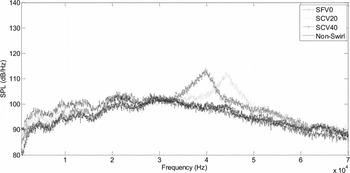
Figure 11. Far-field sound pressure level spectra for Mach number 0.85 and emission angle 90°.
Compared to the L/D=0.5 case, the increase in the pipe length in the case of L/D=2 increases the BSAN level for the non-swirl pipe jet as shown in Fig. 12, for Mach number 1.56. Similarly, the swirl pipe jets also show an increase in the noise levels at L/D=2, compared to L/D=0.5. Increase in the vane angle (or swirl number) also leads to an increase in the noise level. However, BSAN is eliminated in the swirl pipe jets.

Figure 12. Far-field sound pressure level spectra for Mach number 1.56 and emission angle 130°.
The non-swirl pipe jet radiates the maximum noise at all the frequencies, along with screech tone at Mach number 1.83, as shown in Fig. 13. An increase in the vane angle (or swirl number) leads to a reduction in the noise due to increased spread rate and reduction in axial momentum.

Figure 13. Far-field sound pressure level spectra for Mach number 1.83 and emission angle 35°.
4.0 DIRECTIVITY CHARACTERISTICS
The directivity characteristics of swirl and non-swirl pipe jets are discussed in this section for L/D cases of 0.5 and 2 for different Mach numbers.
4.1. Directivity for L/D=0.5
Figure 14 compares the Overall Sound Pressure Level (OASPL) directivity for swirl and non-swirl pipe jets at Mach number 0.85.

Figure 14. Directivity of OASPL for different microphone polar angle Mach number 0.85.
It is observed that the SCV20 pipe jet emanates the least amount of noise at almost all the emission angles among all the swirl and non-swirl pipe jets. The non-swirl pipe jet produces the maximum noise due to the presence of transonic tones at this Mach number. SFV0 jet is noisier than SCV20 and SCV40 pipe jets. As seen in the spectra, the SFV0 pipe jet is energetic in the low frequency range compared to SCV20 and SCV40, which is the reason for the increase in the OASPL levels. Around 8-12dB reduction in OASPL is observed for SCV20 pipe jet compared to non-swirl pipe jet.
However, at Mach number 1.05, the non-swirl pipe jet emits the lowest noise at all the emission angles except at a few downstream angles as shown in Fig. 15. The OASPL levels are lower compared to the Mach number 0.85 case due to the absence of transonic tones. The swirl pipe jets are noisy compared to the non-swirl pipe jets, due to enhanced turbulent mixing between the pipe jet fluid and the ambient. The increase in the turbulent mixing enhances the turbulent mixing noise leading to higher levels of OASPL. An increase in the vane angle increases the mixing in the swirl pipe jets, and consequently, higher OASPLs.

Figure 15. Directivity of OASPL for different microphone polar angle Mach number 1.05.
Upon increasing the Mach number further, the OASPL increases dramatically, by around 15-20dB, due to the presence of shock cells, compared to Mach number 1.05. The non-swirl pipe jet emits the highest noise level at Mach number 1.56 as shown in Fig. 16, except in the emission angle range 40° ≤ EA ≤ 80°, wherein the SCV40 pipe jet emits the maximum noise compared to the other pipe jets. The SFV0 pipe jet emerges as the least noisy jet except at most upstream and downstream angles. Strong shock cells exist at Mach number 1.56 and the shock noise enhances the OASPL level. The upstream noise increments for non-swirl and SFV0 pipe jets are due to the BSAN, which is observed in the spectra. However, the SCV20 and SCV40 pipe jets eliminate the BSAN and are less noisy beyond 120° upstream. Similarly, at the far downstream angles, the SCV20 and SCV40 pipe jets radiate the minimum noise due to the enhancement in spread rate and reduction in the axial momentum.

Figure 16. Directivity of OASPL for different microphone polar angle Mach number 1.56.
For a Mach number of 1.71 (plot not shown here), the non-swirl jet radiates higher noise levels at all the emission angles and SCV40 jet radiates the lowest noise at almost all the emission angles. Similar trend is observed for Mach number 1.83 also with enhanced OASPL compared to M =1.71 (Fig. 17). It is clearly observed that the peak noise is radiated by the non-swirl pipe jet due to the strong shock cells and their interactions with the large-scale turbulence structures. The screech tones also contribute to the increase the OASPL level for the non-swirl pipe jet. However, the screech tone is entirely eliminated by the swirl pipe jets. Similar to the non-swirl pipe jet, the SFV0 and SCV20 pipe jets also emit BSAN (which is observed in the spectra), leading to an increase in the OSAPLs. However, they are less noisy than the non-swirl pipe jet. The SCV40 swirl pipe jet completely eliminates the screech tones and BSAN noise due to the high levels of annular swirl velocity. Hence, SCV40 swirl pipe jet radiates the least noise, except at mid-range emission angles. The noise increments at these mid-range angles are due to the noise emission from the fine-scale turbulence structures, which increases with increase in vane angles.

Figure 17. Directivity of OASPL for different microphone polar angle Mach number 1.83.
4.2. Directivity for L/D=2
Figure 18 presents the directivity at Mach number 0.85 for L/D=2 case. It is observed that SFV0 and SCV20 pipe jets radiate the highest noise levels except at the downstream angles. The presence of the transonic resonance and increase in turbulent mixing causes an increase in the noise level.

Figure 18. Directivity of OASPL for different microphone polar angle Mach number 0.85.
Figure 19 compares the directivity of swirl and non-swirl pipe jets at Mach number 1.56. SFV0 pipe jet emerges the least noisy except at emission angles less than 50°. The reduction in OASPL by SFV0 pipe jet is around 12 dB at mid- and at upstream angles compared to non-swirl pipe jet. However, the reduction in OSAPL levels is smaller towards the downstream angles. The non-swirl pipe jet directivity is almost flat except at upstream angles. The reason behind this is a strong BSAN hump observed for the non-swirl pipe jet at emission angles above 45°.

Figure 19. Directivity of OASPL for different microphone polar angle Mach number 1.56.
At Mach numbers of 1.71 and 1.83, almost similar trends with enhanced OASPL levels are observed. The SCV40 pipe jet radiates lower noise levels at Mach number 1.83 as shown in Fig. 20. This is achieved by the complete elimination of the screech tones and shock associated noise. SFV0 and SCV20 swirl pipe jets come next in noise reduction efficacy. However, at far downstream angles, SFV0 emits screech tone and therefore emits higher noise levels. The upstream forward feedback could not be eliminated by the SFV0 pipe jets at L/D=2.

Figure 20. Directivity of OASPL for different microphone polar angle Mach number 1.83.
4.3. Comparison of L/D
The effects of increasing the pipe lengths on OASPL characteristics are discussed here.
The non-swirl pipe jet of L/D=2 radiates the minimum noise except emission angle less than 50° as shown in Fig. 21. However, the non-swirl pipe jet of L/D=0.5 emits the maximum noise at all the emission angle. This shows the effect of L/D. Around 10dB noise reduction is achieved for non-swirl pipe jet by increasing the pipe length. Similarly, the swirl pipe jets also radiate less noise upon increasing the pipe lengths. The increase in the pipe length causes less entrainment rate and mixing due to the effects of confinement. SCV40 pipe jets reduced the noise around 3-5dB on increasing the pipe lengths.

Figure 21. Directivity of OASPL comparison at Mach number 0.85.
At Mach number 1.56, it is observed that increasing the pipe length of non-swirl pipe jet causes an increase in the noise levels (Fig. 22). This is due to the presence of strong shocks for L/D=2 case, compared to L/D=0.5 case. The swirl pipe jets follow the trend of decrease in the noise levels with an increase in the pipe lengths, as observed in Mach number 0.85. SFV0 pipe jet does not show BSAN hump for L/D=2 and thus leads to low noise levels compared to L/D=0.5 case. SFV0 pipe jet of L/D=2 radiates less noise compared to other pipe jets.

Figure 22. Directivity of OASPL comparison at Mach number 1.56.
However, at Mach number 1.83, the non-swirl pipe jets radiate the same amount of noise irrespective of the pipe lengths, as shown in Fig. 23. Similarly, SFV0 pipe jets also emit almost the same amount of noise at upstream angles, although at mid-range angles, around 2dB difference is observed. However, SCV40 swirl pipe jet radiates the least noise for L/D=2. The emission of Mach wave is suppressed for the co-axial pipe jets due to the suppression of convective velocity of the eddies in the primary shear layers(Reference Rostamimonjezi20) and leads to lower noise radiation compared to non-swirl pipes.

Figure 23. Directivity of OASPL comparison at Mach number 1.83.
5.0 FLOW FIELD CHARACTERISTICS
This section deals with the centreline total pressure (Pt ) measured along the centreline of the jet using pitot tube. In the case of under-expanded jets, the probe measures the pressure behind the shocks and thus, at such conditions, the results are merely qualitative. However, the results indicate the overall shock cell structures, number of shock cells, shock cell spacing, axial extent of the core lengths, for comparison of the different jets. Further, the centreline pressure decay is an indirect measure of the mixing(Reference Phanindra, Chiranjeevi and Rathakrishnan25). Hence, the mixing characteristics of different pipe jet models also can be compared from this study.
5.1. Centreline total pressure variation for L/D=0.5
The non-swirl pipe jet shows the maximum core length compared to other pipe jets for Mach number of 0.85 (Fig. 24). For SFV0 and SCV40 pipe jets, almost no core length is exhibited, and decay follows.

Figure 24. Centreline total pressure variation at Mach number 0.85.
The rapid mixing in the case of SCV40 jet does not extend in the downstream locations, whereas SCV20 jet shows better decay. Nevertheless, SCV20 and SCV40 jets show rapid decay in the near field. The reduction in core length with increase in vane angle is due to the enhanced entrainment and mixing.
Figure 25 shows that maximum core length for the non-swirl pipe jet at Mach number 1.56, wherein the core shows a series of shock cells up to x/D=8. These shock cells generate maximum noise in the non-swirl pipe jet at Mach number 1.56 compared to the other pipe jets. However, the swirl pipe jets eliminate the shock cells with a reduction of the core length compared to non-swirl pipe jet. The addition of swirl components destroy the shock cells and increase the entrainment rate (radially outwards), which helps to equilibrate the jet pressure with the ambient pressure faster compared to non-swirl pipe jet. Thus, it is evident that the noise reduction at Mach number 1.56 for the swirl pipe jets is due to the destruction of the shock cells.

Figure 25. Centreline total pressure variation at Mach number 1.56.
The increase in Mach number to 1.83 causes strong shocks and more number of shock cells for the non-swirl pipe jet as shown in Fig. 26. The axial extent of the pressure oscillations in the non-swirl pipe jet is until x/D=14, which is more than that for Mach number 1.56. In a similar trend, for SFV0 and SCV20 swirl pipe jets, the shock cells are observed until x/D=8. The shock oscillations and number of shock cells are less for the swirl pipe jets compared to the non-swirl pipe jet. However, for SCV40 swirl pipe jet, the shock cells are not observable from the centreline pressure data. An increase in the vane angle causes reduction in the number of the shock cells for the swirl pipe jets compared to non-swirl jet. A strong pressure deficit is observed for SCV40 swirl pipe jets, due to fact that pressure equilibration occurs across a fewer number of shock cells or with strong shocks. Hence, a strong Mach disk is generated in order to match the pipe jet pressure with the ambient. The flow visualisation study also confirms this observation. Now, it is clear why swirl pipe jets radiate the lower noise levels compared to non-swirl pipe jet at higher Mach numbers.

Figure 26. Centreline total pressure variation at Mach number 1.83.
5.2. Centreline total pressure variation for L/D=2
The increase in pipe length elongates the core length for L/D=2 case, compared to L/D=0.5 case as shown in Fig. 27. The mixing and decay of the SFV0 and non-swirl pipe jets are lower compared to SCV20 and SCV40 swirl pipe jets. The addition of the swirl always helps to increase the mixing rates, but enhances the turbulent mixing noise.

Figure 27. Centreline total pressure variation at Mach number 0.85.
The non-swirl pipe jet exhibits a shock cell length of around x/D=6 for Mach number 1.56 (Fig. 28). The fluctuations are strong and higher, leading to strong BSAN levels, as observed in the spectra for L/D=2 (Fig. 12) compared to the L/D=0.5 (Fig. 8). The swirl pipe jets demonstrate a reduction in core lengths and destruction of the shock cells compared to non-swirl pipe jets.

Figure 28. Centreline total pressure variation at Mach number 1.56.
At Mach number 1.83, the non-swirl pipe jet shows a series of shock cells until x/D=11, as observed in Fig. 29, which is less compared to L/D=0.5 case. Similarly, shock cell length reduction is observed for SFV0 and SCV20 swirl pipe jets compared to L/D=0.5 case. However, the SCV40 swirl pipe jet seems to behave the same for both the cases.

Figure 29. Centreline total pressure variation at Mach number 1.83.
It is clear that increase in pipe length causes a decrease in the core lengths and an increase in the BSAN in the spectra. Further, it is evident that increase in the pipe length (L/D=2) reduces the core length and increases the shock strength or BSAN compared to L/D=0.5.
6.0 FLOW VISUALISATION
This section discusses the schlieren photographs captured for the non-swirl and swirl pipe jets at Mach numbers 1.56 and 1.83. Since the shock associated noise is a major noise component at supersonic conditions and this study can reveal the nature of shock cells, number of shock cells and strength of the shocks.
6.1. Schlieren photographs for L/D=0.5
Figure 30 shows the schlieren photographs for Mach number 1.56 for the non-swirl and swirl pipe jets. Series of shock cells are observed for the non-swirl pipe jet due to the pressure difference between the pipe jet fluid and the ambient. However, for the swirl pipe jets, the shock cells are attenuated and a reduction in the shock cell length is observed. An increase in the vane angle leads to enhanced destruction of the shock cells. Besides vane angle, the secondary jet also plays a role in the mitigation of the shock cells.

Figure 30. Schlieren photographs at Mach number 1.56, L/D=0.5.
The increase in Mach number causes strong shock cells to be generated for non-swirl pipe jet as shown in Fig. 31, at a Mach number of 1.83. A strong Mach disk usually appears for free jets around Mach number 1.56(Reference Rathakrishnan26). However for the non-swirl pipe jet, a very small Mach disk is observed. However, the Mach disk is clearly observed for the swirl pipe jets due to elimination of the shock cells and the need for a strong shock to equalise the pressure. SFV0 and SCV20 swirl pipe jets also display a series of complex shock patterns, although for a shorter distance. The presence of the vanes in the annular passage at an angle and the swirl flow from these passages interacts with the primary jets, which generates a complex shock cell pattern. A reduction in the shock cell length and the number of shock cells are clearly observed for the swirl pipe jets compared to non-swirl pipe jet.

Figure 31. Schlieren photographs at Mach number 1.83, L/D=0.5.
6.2. Schlieren photographs for L/D=2
Figure 32 shows the schlieren photographs for Mach number 1.56, L/D=2. A Mach disk is observed for the swirl pipe jets at Mach number 1.56; however, no Mach disk is observed for the non-swirl pipe jet. This might be due to the confinement effect and suppression of the expansion fans from the primary jet by the secondary jet. However, at Mach number 1.83, a Mach disk is observed for the non-swirl pipe jet as shown in Fig. 33. For the swirl pipe jets, the expansion waves in the secondary core reflect from the interface between the primary and secondary jets and this generates a separate set of shocks near the first shock cell. The same behaviour was reported by Baek et al(Reference Baek, Kwon and Lee27) for a supersonic dual co-axial free jet.

Figure 32. Schlieren photographs at Mach number 1.56, L/D=2.

Figure 33. Schlieren photographs at Mach number 1.83, L/D=2.
From the schlieren photographs, it is evident that application of co-axial swirl in the pipes leads to a weak shock cell system and therefore much lower shock associated noise levels compared to non-swirl pipe jets.
7.0 CONCLUSIONS
An experimental study has been carried out on the acoustic far fields and flow features of the confined co-axial swirl pipe jets. The application of swirl reduces the OASPL levels by around 8–12dB compared to non-swirl jet at Mach number 0.85 for L/D=0.5. The swirl entirely eliminates the screech tones and mitigates the shock associated noise at supersonic conditions. At Mach number 1.56 for L/D=2, noise reduction of around 12dB is achieved by the SFV0 pipe jet at mid- and at upstream angles compared to non-swirl pipe jet. However, at Mach number 1.83, both SFV0 and SCV40 swirl pipe jets are efficient in noise suppression for both the L/D cases. Increase in the pipe length causes a reduction in the OSAPL at a Mach number of 0.85, while enhance the noise at supersonic Mach number of 1.56, for the non-swirl jet. However, the swirl pipe jet reduces the noise upon increasing the pipe length for the Mach numbers of 0.85 and 1.56. Reduction in the core lengths and steep centreline pressure decay are observed for the swirl pipe jets compared to non-swirl pipe jets for all the Mach numbers tested. The weakening/destruction of the shock-cell increases with increase in the vane angle.


