2.0 THE SPECIFIC RANGE METHOD FOR FLIGHT MONITORING

The method is based on monitoring the aircraft specific range during cruise flight by measuring flight speed and fuel flow and comparing the results with flight manual data^{(Reference Speyer1)}. The specific range is an index that shows the relationship between flight distance and fuel consumed in a cruise flight segment. It is a measure of the aircraft efficiency and is usually expressed by the distance in nautical miles [NM] per fuel mass [kg].

(2)\begin{equation} \begin{gathered} SR = \frac{Distance}{Fuel Mass}=\frac{V \cdot dt}{FF \cdot dt}=\frac{V}{FF} \end{gathered}\end{equation}

Analysing Eq. (2) the specific range value varies with flight speed (V) and engine fuel flow (FF). At low speeds, the aircraft flies at high angle-of-attack (α), high lift coefficient (CL) and consequent high drag coefficient (CD), which increases fuel flow, resulting at low specific range. At high speeds, the drag is also increased with compressibility effect and high dynamic pressure, therefore the specific range is also reduced. Inside most of the flight envelope there is an intermediate value of flight speed that results at the maximum specific range. This is the Maximum Range Cruise and usually cruise flight is always performed near this economical speed.

In Fig. 1, the specific range variation with speed is shown for a specific cruise condition (Weight, Altitude and Temperature), the maximum range speed is near 150 KIAS and the upper speed boundary is limited by maximum operational speed (VMO/MMO), by maximum cruise thrust or buffet boundary. The lower boundary is usually limited by minimum flight speed regarding stall or buffet margins.

Figure 1. Specific range as a function of indicated cruise speed.

Using this concept of specific range, monitoring flight efficiency follows a systematic process of analysing flight measured data together with the aircraft theoretical drag polar and engine map.

The process is divided in two steps. The first consists of taking flight measured parameters from the aircraft instrumentation system, and the second is the calculation of three different specific ranges using flight manual, drag polar and the engine map⁽⁵⁾.

1. 1. Measure aircraft true flight speed (VT).

2. 2. Measure aircraft fuel flow (FF_m).

3. 3. Measure or estimate the aircraft weight (W).

4. 4. Measure engines parameters: rotation speed (N1), pressure ratio (EPR), torque (TQ),

5. 5. Measure atmospheric parameters (Altitude H_p and Temperature OAT),

6. 6. Calculate the correct specific range (SR_c),

   (3)\begin{equation}\begin{gathered} SR_c = \frac{VT}{FF_m} \end{gathered}\end{equation}

7. 7. With the flight measured parameters W, H_p, OAT, VT, and wing area S and with theoretical drag polar, calculate the lift and drag coefficient (CL, CD),

   (4)\begin{equation}\begin{gathered} CL = \frac{2 \cdot W}{\rho \cdot S \cdot VT^{2}} \\ CD = f(CL,Mach) \end{gathered}\end{equation}

8. 8. Calculate the Drag or theoretical thrust,

   (5)\begin{equation}\begin{gathered} Drag = \frac{1}{2} \cdot \rho \cdot S \cdot VT^{2} \cdot CD \\ \textit{In Cruise Conditions:} \\ Drag = Thrust \end{gathered}\end{equation}

9. 9. With the theoretical Thrust, H_p, OAT and VT and using the information included in the engine map, find the theoretical aerodynamic fuel flow (FF_a).

10. 10. Calculate the aerodynamic specific range (SR_a),

    (6)\begin{equation} \begin{gathered} SR_a = \frac{VT}{FF_a} \end{gathered}\end{equation}

11. 11. With the measured engine parameters (N1, EPR, TQ), H_p, OAT and VT, find the theoretical engine fuel flow (FF_e) according to the engine map.

12. 12. Calculate the engine specific range (SR_e),

    (7)\begin{equation}\begin{gathered} SR_e = \frac{VT}{FF_e} \end{gathered}\end{equation}

These steps allow the distinction between aircraft performance behaviour due to aerodynamic or engines deterioration by comparing the three specific ranges (SR_c, SR_a and SR_e). An example of this process for aircraft with turbofan engines with N1 as the engine monitoring variable is shown in Fig. 2.

(8)\begin{equation} \begin{gathered} \Delta Global = \frac{SR_c}{SR_a} \\[3pt] \Delta Engine = \frac{SR_c}{SR_e} \\[3pt] \Delta Aerodynamic = \frac{SR_e}{SR_a} \\ \end{gathered}\end{equation}

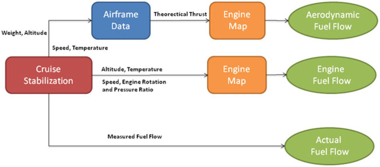
Figure 2. The specific range monitoring process⁽⁵⁾.

In Eq. (8) the calculated ΔGlobal is the difference of the aircraft corrected specific range, calculated with the actually measured aircraft fuel flow, in relation to the original flight manual predicted value, calculated with the fuel flow estimated in engine map with the predicted aircraft thrust using the AFM drag polar. This resulting factor is an index on how much the more fuel aircraft is burning due to airplane deterioration, and it should be used in flight planning to update predicted block fuel and also economic flying speeds. The index ΔEngine and ΔAerodynamic are factors that account for the effect of the engine and aerodynamic deteriorations respectively on the total global specific range difference. These should be used as metrics to enhance maintenance planning.

2.1 The specific range method disadvantages

Although this method is widely used as the main tool for cruise performance monitoring, there are some concerns regarding its use. The two problems on using this method are some sources of scatter and biases on the flight parameters measurements that may cause misinterpretation of the results, and the tight cruise stabilisation criteria necessary to correctly apply this method since it does not account for accelerations, changes in altitude and other flight transients. The source of scatter and biases are⁽⁴⁾:

• Fuel heating value

• Aircraft gross weight

• Sensors accuracy and scatter

• CG position

• N1/EPR ratios

• Atmospheric influences

The airplane performance and fuel consumption is directly related to the amount of energy the fuel releases after combustion. This energy content is measured by the fuel heating value. Usually, flight manual and engine performance maps uses an average value in its fuel flow tables. Depending on fuel storage management and atmospheric properties, the heating value may vary, and this reflects on the aircraft fuel consumption, as seen in Fig. 3. A good practice for flight operations engineering is to measure these fuel properties constantly and apply corrections to the performance monitoring results due to the differences in the heating value.

Figure 3. Fuel heating value variation with fuel density⁽⁵⁾.

If an airline keeps track of its fuel density with routine measurements, the fuel flow factor due to lower heating value (LHV) variation is shown in Eq. (9).

(9)\begin{equation}\begin{gathered} \frac{\Delta FF}{FF_{REF}} = -\frac{\Delta LHV}{LHV_{REF}} \\[3pt] \frac{\Delta SR}{SR_{REF}} = \frac{\Delta LHV}{LHV_{REF}} \\ \end{gathered}\end{equation}

The aircraft gross weight is a source of uncertainty on aircraft monitoring due to passengers and cargo weight scattering during flight and basic operational weight variations. It is customary during flight operations to consider standard values for each passenger, baggage and cargo weights, these values are derived from international regulations that compile distributions of weights among group of passengers to be used by airlines. The variations on basic operational weight (BOW) is explained by dirt accumulation both internally and externally, addition of new equipments, structural repairs and old paintings. A trend of 0.2% increase in BOW is expected for the first ten years of aircraft operation⁽⁴⁾. This weight uncertainty that promotes bias and scatter on the results of the performance monitoring are reduced on modern aircrafts and avionic systems that have an indirect measurement of in-flight weight, by combining measurements such as angle-of-attack and vertical acceleration, the actual weight is predicted. Although less uncertainty is expected, sensors scatter still can produce misinterpretation on the specific range monitoring results.

The variations in CG position in flight will result in additional scatter and source of uncertainty due to the effect of CG position on aircraft total drag. In flight CG monitoring is possible and may improve flight planning and monitoring results.

Engine rotational speed (N1), pressure ratio (EPR) and torque (TQ) values are the measured parameters that relates to the thrust performance. Different engines may present different relations between these parameters and the actual thrust. The value published in engine performance manuals are based on the average of the N1/EPR/TQ to thrust (T) ratios for a new engine. Aging engines have their performance deteriorated and corrections must be applied to account for these different ratios and correct interpretations of specific range monitoring.

Besides these sources of uncertainty in performance monitoring results, other practical difficulty on using this method is the perfect stabilisation assumption the method applies which are difficult to encounter on every cruise flight. In order to assume a stabilised flight, these conditions shall be met for at least 3 continuous minutes⁽⁶⁾:

• Altitude changes in the range of ± 25ft

• Ground speed in the range of ± 1kn

• Heading angle changes less then 5°

• Roll angle less then 1°

• Air temperature in the range of ±1°

• No turbulence

Usually after a cruise stabilisation segment, the specific range is measured at each time and an adjusted function is fitted to the measured data.

In Fig. 4 the average specific range for this cruise stabilisation is of 0.2845NM/kg and the standard deviation is of 0.0013NM/kg. Therefore, assuming a Gaussian distribution, the value of the specific range for this specific flight condition is between [0.2819 – 0.2871] with a 95% confidence interval (2σ).

Figure 4. Measured and fitted specific range for a cruise stabilisation.

These sources of uncertainty, scatter, biases and also the practical difficulty of a perfect stabilisation in cruise may be reduced by filtering techniques applied to raw measurements and mathematical modelling accounting for accelerations, measurements and process noise.

3.0 UNSCENTED KALMAN FILTER

The Kalman filter is a powerful tool to predict and identify aircraft states and parameters in the time domain. The use of the filter has the advantage of using dynamic equations to predict aircraft states and measurements information to update predictions according to the state and observations covariance matrix. The traditional Kalman filter is the optimal filtering estimation technique for a linear dynamic model^{(Reference Kalman7)}. For the cases of nonlinear equations such as for the aircraft equations of motion, an approximation for the linear Kalman filter must be applied in order to use the linear filter to nonlinear models. The general form of the nonlinear model used in the state estimation is:

(10)\begin{equation} \begin{gathered} \dot{\mathbf{x}}=f(\mathbf{x},\mathbf{u},\mathbf{w}) \\ Y = g(\mathbf{x},\mathbf{u},\mathbf{v}) \end{gathered}\end{equation}

In Eq. (10) the vector X is the state variables, Y are the observable values and u are the control inputs. The values of w and v are the state and measurements noise vectors with covariances Q and R.

The two mostly common adaptation of a linear Kalman filter to a non-linear dynamic model are the extended and unscented filters.

The extended Kalman filter (EKF) consists of linearising around the predicted state, at each integration step, the non-linear state equations to correct the state covariance matrix using the linear Kalman filter approach. The observation dynamic model is also linearised at each step to calculate the Kalman gain matrix and update the state predicted values.

The unscented Kalman filter (UKF) consists of approximating the nonlinear dynamic model with a sample point distribution of sigma-points (χ) via an unscented Transformation^{(Reference Wan and van der Merwe8)}.

In this work, the unscented Kalman filter is applied as it provides a better approximation of the non-linear dynamic model since the EKF uses a Taylor expansion up to the first order for the linearisation, while the UKF approximation are accurate to at least the second order^{(Reference Wan and van der Merwe8)}.

Considering a state variable vector X with dimension L and covariance matrix P_x(X, W), the sampled distribution of sigma-points and associated pondering factors for the mean (W^m) and covariance (W^c) are:

(11)\begin{equation}\begin{gathered} \chi_{0}=\overline{\mathbf{x}} \\ \chi_{i}=\overline{\mathbf{x}} \pm (\sqrt{(L+\lambda)P_{x}})_{i} \quad i=1:L \\ W_{0}^m=\frac{\lambda}{L+\lambda} \\ W_{0}^c=\frac{\lambda}{L+\lambda}+(1-\alpha^2+\beta) \\ W_{i}^{m,c}=\frac{1}{2(L+\lambda)} \\ \lambda=\alpha^2L-L \end{gathered}\end{equation}

The variables α, β are sigma-point distribution free parameters and for this work assumes the values of 0.01 and 2 respectively.Once the sigma-point are computed, the state and covariance matrix can be propagated using the augmented state χ.

(12)\begin{equation} \begin{gathered} \dot{\chi_{p}}=f(\chi,\mathbf{u}) \\ \mathbf{x}_{p}=\sum_{i=0}^{i=L}W_{i}^{m}\chi_{p} \\ P_{x}=\sum_{i=0}^{i=L}W_{i}^{c}(\chi_{p}-\mathbf{x}_{p})(\chi_{p}-\mathbf{x}_{p})^{T}+Q \\ Y_{i}=g(\chi_{p},\mathbf{u}) \\ \mathbf{y}_{p}=\sum_{i=0}^{i=L}W_{i}^{m}Y_{i} \\ P_{y}=\sum_{i=0}^{i=L}W_{i}^{c}(Y_{p}-\mathbf{y}_{p})(Y_{p}-\mathbf{y}_{p})^{T}+R \\ P_{x,y}=\sum_{i=0}^{i=L}W_{i}^{c}(Y_{p}-\mathbf{y}_{p})(\chi_{p}-\mathbf{x}_{p})^{T} \\ \end{gathered}\end{equation}

The propagated states and covariance matrix may be updated with the information of the observable variables Z weighted by the Kalman gain matrix K.

(13)\begin{equation} \begin{gathered} K=P_{x,y}P_{y}^{-1} \\ \mathbf{x}_{a}=\mathbf{x}_{p}+K(Z-\mathbf{y}_{p}) \\ P_{x_{a}}=P_{x}-KP_{x,y}^{T} \end{gathered}\end{equation}

The updated state variable X_a and covariance matrix P_xa is the best estimate of the state x and P_x and the unscented process is repeated following these steps beginning in Eq. (11) until the end of observations.

In Fig. 5 the benefit of using an unscented Kalman filter procedure for state identification is outlined by showing the better covariance prediction when compared to the first order linearisation in an extended Kalman filter process also used for non-linear models.

Figure 5. Example of mean and covariance propagation^{(Reference Wan and van der Merwe8)}.

3.1 Noise and process covariance matrix R and Q

The noise covariance matrix Q and R are parameters sensitive to the filter convergence and must be set accordingly to improve the filter results.These parameters affects the Kalman gain matrix K in a way that if the observation noise R is high, the Kalman matrix will be small, therefore the updated state X_a will be similar to the predicted value X_p. If the noise covariance R is low or the process noise Q is high, the updated state X_a will be corrected by the innovation sequence gain K(Z - y_p).

In this work, the observations covariance matrix R was set using a Fourrier smoothing^{(Reference Morelli9)} through all measured variables. The variance of the output noise signal is the R_i,i element of the noise covariance matrix.

In the specific example of angle-of-attack signal in Fig. 6(b), the element υ_i,i of the noise covariance matrix R is 5.6 · 10⁻⁴ degree corresponding to an angle-of-attack standard deviation of 0.024° .

Figure 6. Measurement noise covariance.

For the process noise covariance matrix Q, an adaptive procedure based on covariance matching was implemented during the unscented Kalman filter process^{(Reference Akhlaghi, Zhou and Huang10, Reference Shyam Mohan, Naik, Gemson and Ananthasayanam11)}. The process noise w_k may be approximated by the difference between the updated state X_a and the predicted value X_p.

(14)\begin{equation}\begin{gathered} w_{k}=\mathbf{x}_{a}-\mathbf{x}_{p}\\ \mathbf{x}_{a}-\mathbf{x}_{p}=K(Z-\mathbf{y}_{p}) \\ w_{k}=K(Z-\mathbf{y}_{p}) \\ Q=Cov(w_{k})=K[Cov(Z-\mathbf{y}_{p})]K^{T} \\ [Cov(Z-\mathbf{y}_{p})]=\frac{1}{N_{Q}}\sum_{i=1}^{i=N_{Q}}(Z-\mathbf{y}_{p})(Z-\mathbf{y}_{p})^{T} \\ \end{gathered}\end{equation}

In Eq. (14) the parameter N_Q is the process noise updating window. In this work, a window of 200 observations was used to update the state process covariance matrix Q.

4.0 FLIGHT PERFORMANCE MONITORING

For cruise flight monitoring using the unscented Kalman filter approach, a state and measurement model has to be defined. The strategy for identifying the specific range ratios between aircraft current performance with the aerodynamic and engine database such as in Eq. (8) are setting these ratios as pseudo-states in the filter state model. Additionally to these parameters, a drag and lift coefficient was also identified during the filtering process.

4.1 The state equations model

The aircraft dynamics in cruise flight phase may be approximated by its longitudinal model only. The dynamic equations modelled in this work are in the body reference frame as in Fig. 7 and the states considered are the inertial speed in the X, Y and Z axis u, v and w, the flight geometric altitude H_g, pitch and flight path angle θ and γ, angle-of-attack ±, sideslip β and pitch rate q. The pseudo-states to be identified are the drag and lift coefficient CD and CL, the wind speed in the north axis (VwN) and east directions (VwE), the fuel flow ratios $K_{FF_{1}}$ and $K_{FF_{2}}$ for the left and right engines in relation to the engine manufacturer database and $K_{FF_{a_{1}}}$ and $K_{FF_{a_{2}}}$ relating to the aerodynamics theoretical required thrust.

(15)\begin{equation}\begin{gathered} \dot{u}=\frac{-mg \cdot sin(\theta) + T \cdot cos(\epsilon)+F_{X_{Body}}-q \cdot w}{m} \\[1.5pt] \dot{v}= \frac{mg \cdot cos(\theta) \cdot sin(\phi) + F_{Y_{Body}}}{m} \\[1.5pt] \dot{w}=\frac{mg \cdot cos(\theta) \cdot cos(\phi)+ T \cdot sin(\epsilon)+F_{Z_{Body}}+q \cdot u}{m}\\[1.5pt] \dot{h}= -(-sin(\theta) \cdot u + sin(\phi) \cdot cos(\theta) \cdot v + cos(\phi) \cdot cos(\theta)\cdot w) \\[1.5pt] \dot{\theta}= q \\[1.5pt] \dot{\alpha} = \frac{u_{w} \cdot \dot{w}-w_{w} \cdot \dot{u}}{u_{w}^{2}} \cdot cos(\alpha)^{2} \\[1.5pt] \dot{\beta} =\frac{V_{T} \cdot \dot{v} - v_{w} \cdot \dot{V_{T}}}{cos(\beta) \cdot V_{T}^{2}} \\[1.5pt] \dot{\gamma}=q-\dot{\alpha}\\[1.5pt] \dot{q}= 0 \\[1.5pt] \dot{CD}= 0 \\[1.5pt] \dot{CL}= 0 \\[1.5pt] \dot{K_{FF_{1}}}= 0 \\[1.5pt] \dot{K_{FF_{2}}}= 0 \\[1.5pt] \dot{K_{FF_{a_{1}}}}= 0 \\[1.5pt] \dot{K_{FF_{a_{2}}}}= 0 \\[1.5pt] \dot{V_{w}N}= 0 \\[1.5pt] \dot{V_{w}E}= 0 \end{gathered}\end{equation}

Figure 7. NED and body reference system with Euler angles.

In Eq. (15) the variables $[u_{w}, v_{w}, w_{w}]$ are the true airspeed (V_T) in the body reference frame, these speeds, the angle-of-attack (±) and sideslip (β) are defined as follows:

(16)\begin{equation}\begin{gathered} \alpha=atan\left(\frac{w_{w}}{u_{w}}\right) \\ \beta=asin\left(\frac{v_{w}}{V_{T}}\right) \\ u_{w} = u+wind_{x} \\ v_{w} = v+wind_{y} \\ w_{w} = w+wind_{z} \\ V_{T} = \sqrt{u_{w}^{2}+v_{w}^{2}+w_{w}^{2}} \\\end{gathered}\end{equation}

The wind speed in the body reference frame $[wind_{x}, wind_{y}, wind_{z}]$ and the forces $[F_{X_{Body}}, F_{Y_{Body}}, F_{Z_{Body}}]$ are calculated by rotations matrix between NED and wind to body reference frames respectively ($L_{NED_{to}Body}, L_{Wind_{to}Body})$.

(17)\begin{equation}\begin{gathered} \begin{bmatrix} wind_{x} \\[3pt] wind_{y} \\[3pt] wind_{z} \end{bmatrix} =L_{NED_{to}Body} \cdot \begin{bmatrix} V_{w}N \\[3pt] V_{w}E \\[3pt] 0 \end{bmatrix} \\[5pt] \begin{bmatrix} F_{X_{Body}} \\[3pt] F_{Y_{Body}} \\[3pt] F_{Z_{Body}} \end{bmatrix} =L_{Wind_{to}Body} \cdot \begin{bmatrix} -D \\[3pt] 0 \\[3pt] -L \end{bmatrix}\end{gathered}\end{equation}

During the state estimate model, some parameters are not modelled and enter the dynamic equations as control inputs. They are the engine thrust T, RPM and torque, the aircraft CG position and atmospheric temperature OAT.

4.2 Observation model

As an observation model, the aircraft instrumentation system is used to enhance the observability of the dynamic equations. The measured variables Z are the GPS/Inertial ground speeds in the north, east and vertical axis [VN, VE, VZ], the aircraft inertial attitude [θ] and pitch rate [q], the angle-of-attack measured by the aircraft clinometry system [±], the true airspeed and pressure altitude [VT, H_p] measured by the anemometric data and the measured fuel flow [$FF_{1_{m}}$, $FF_{2_{m}}$].

(18)\begin{equation}\begin{gathered}\begin{bmatrix} \mathbf{y(1)} = VN \\[3pt] \mathbf{y(2)} = VE \\[3pt] \mathbf{y(3)} = VZ \end{bmatrix} =L_{Body_{to}NED} \cdot \begin{bmatrix} u \\ v \\ w \end{bmatrix} \\[3pt] \mathbf{y(3)}= \mathbf{x(3)} \cdot \frac{T_{ISA}}{OAT} = H_{p} \\[3pt] \mathbf{y(4)}= \mathbf{x(5)} = \theta \\[3pt] \mathbf{y(5)}= \mathbf{x(4)} = \alpha \\[3pt] \begin{bmatrix} \mathbf{y(6)} = VT \\[3pt] \mathbf{y(7)} = 0 \\[3pt] \mathbf{y(8)} = 0 \end{bmatrix} =L_{Body_{to}Wind} \cdot \begin{bmatrix} u_{w} \\ v_{w} \\ w_{w} \end{bmatrix} \\[3pt] \mathbf{y(9)}= K_{FF_{1}} \cdot FF_{1}=FF_{1_{m}} \\[3pt] \mathbf{y(10)}= K_{FF_{2}} \cdot FF_{2}=FF_{2_{m}} \\[4pt] \mathbf{y(11)}= K_{FF_{a_{1}}} \cdot FF_{a_{1}}=FF_{1_{m}} \\[3pt] \mathbf{y(12)}= K_{FF_{a_{2}}} \cdot FF_{a_{2}}=FF_{2_{m}} \\[3pt] \end{gathered}\end{equation}

During the filtering and estimation process, the theoretical aerodynamic data (CL_REF, CD_REF) are calculated in order to compare these values that were used to calculate the AFM data with the predicted state results (CD, CL).

(19)\begin{equation}\begin{gathered} CL_{REF} =f(\alpha,CG,CT) \\ CD_{REF} =f(\alpha,CG,CT) \\ CT=\frac{T}{qS} \\ \end{gathered}\end{equation}

The fuel flow data [FF ₁, FF ₂, FF_{a 1}, FF_{a 1}] used during the state update process are calculated with the engine databank as a function of rotation speed RPM, torque, temperature, altitude and airspeed.

(20)\begin{equation}\begin{gathered} FF =f(\Delta ISA,H_{p},RPM,Torque,VT) \\ \Delta ISA=OAT-T_{ISA} \\ VT=\mathbf{y(6)}\\ H_{p}=\mathbf{y(3)} \end{gathered}\end{equation}

In Eq. (20) the values of the fuel flow using the engine databank and the aerodynamic reference thrust (FF ₁/FF ₂ and FF_{a 1}/FF_{a 2}) are calculated by adjusting the measured engine torque by the relation between the reference and the identified drag coefficients (CD_REF and CD).

5.0 MONITORING RESULTS

The results of the filtering process is shown for an adaptive window for the states noise covariance matrix Q of 200 test points. These results are for a cruise stabilisation at a weight of approximately 20,000kg, at FL050 and constant speed of 160kts.The measured and estimated ground speeds (in north: VN, in east: VE and vertical: VZ) are shown in Fig. 8.

Figure 8. Identified aircraft speeds.

The aircraft pitch angle (θ), angle-of-attack (±) and flight path (γ) are also identified in Fig. 9. The pitch and angle-of-attack are states with associated measurements, while the flight path angle for this cruise stabilisation is calculated as the difference between the pitch and angle-of-attack.

Figure 9. Identified aircraft angles.

The pressure altitude (H_p) and true airspeed (V_T) are also identified and compared to the measured parameter from the calibrated anemometric system in Fig. 10.

Figure 10. Identified pressure altitude and true airspeed.

The additional state parameters estimated by the use of the filtering process during the performance monitoring are the wind speed in the north and east directions and the sideslip angle as seen in Fig. 11.

Figure 11. Identified wind speeds and sideslip angle.

The most important state parameters identified as a result of the cruise monitoring process are the fuel flow factors $K_{FF_{1}}$, $K_{FF_{2}}$, $K_{FF_{a_{1}}}$ and $K_{FF_{a_{2}}}$ and the lift and drag coefficients CL, CD.

In Table 1, these identified states are shown with the associated standard deviations. The average specific range using the filtered result is 0.2840 with a standard deviation of 0.0004, therefore within a 95% confidence interval, the specific range for this stabilisation lies within [0.2832 – 0.2848]. This result proves the better reliability of the filtered outputs when compared to the specific range monitoring method with the result of 0.2845 ± 0.0013.

Table 1 Identified Aircraft States

The aerodynamic results are compared in Table 2 with the reference drag and lift used to develop the aircraft flight manual AFM.

Table 2 Aerodynamic Comparison

When analysing the results in Table 2, the percentage difference in CL and CD are accompanied by the difference in the lift to drag ratio, L/D. This fact reduces the probability of being an anemometry offset as the difference in the L/D ratio is related to the thrust to weight ratio (T/W) of the aircraft in this flight situation, therefore it means that to sustain a constant speed cruise, the aircraft needs more thrust or is at a higher weight than predicted.

The effect of weight may be further analysed when looking at the CL results; the difference is −0.3%, and during cruise phase, an offset in CL is followed by the same offset in weight, since these two variables are linearly linked. Since the L/D bias is +3%, and this is the same as a 3% increase in the W/T ratio, it is an indicative that at this flight condition, the offset in the aerodynamic efficiency is due to the drag bias (CD) and not to a lift decrement due to a possible error in aircraft weight estimation.

When calculating the specific range (SR), the overall difference is 1.78% meaning that the performance of the aircraft is almost 2% better than the predicted model. This difference is divided into two main effects, the engine and aerodynamic state of the aircraft.

Due to the better engine fuel flow behaviour in this flight conditions, the difference when considering only the engine performance would be 3.36%, but the higher drag coefficient encountered (+3.13%) in this flight condition contributes negatively to the specific range difference, this difference in CD reduces the specific range offset by 1.55% culminating at the overall 1.78% improvement in the aircraft specific range in this flight condition.

These specific range factors were calculated during the filtering process using the following procedure in Eq. (21).

(21)\begin{equation}\begin{gathered} SR_{c} = \frac{VT}{FF_{m}}=\frac{VT}{K_{FF_{1,2}} \cdot FF_{e}}= \frac{VT}{K_{FF_{a_{1,2}}} \cdot FF_{a}} \\ \Delta Global = \frac{1}{K_{FF_{a_{1,2}}}} \\ \Delta Engine = \frac{1}{K_{FF_{1,2}}} \\ \Delta Aerodynamic = \frac{K_{FF_{a_{1,2}}}}{K_{FF_{1,2}}} \\ \end{gathered}\end{equation}

6.0 CONCLUSION

In this work the aircraft performance monitoring process was explored by comparing the traditional specific range method with an application of an optimal filtering process identification using Newton’s second law in the body X, Y and Z axis. Besides the fuel flow factors of a traditional fuel monitoring process, the optimal filtering method had also as an output, the aerodynamic characteristics of the aircraft such as the drag and lift coefficient (CD and CL), the wind speeds and sideslip angle which can be further used to correlate the fuel factor to aircraft deterioration or weight increase. The use of this approach presents a methodology to enhance fleet performance auditing by linking airline operational monitoring results to airframe and engine maintenance schedules. For future work and research, the use of other types of nonlinear filters, such as the particle filtering and ensemble Kalman (EnKF) may be explored together with the study of different strategies for filter adaptation of the process covariance matrix Q and the results compared with the more traditional unscented and extended Kalman filters. The use of more complex filtering techniques and adaptation algorithms tend to further relax the stabilisation criteria and increase the results robustness to sensor scatter. Besides the cruise monitoring presented in this work, the climb and descent flight phases may also be monitored using a similar approach as the proposed method does not assume a stabilised cruise phase as the traditional specific range method requires. The monitoring of climb and descent phases have a greater importance for regional aircrafts which fly in shorter routes where the climb and descent optimisation play an important role on the overall flight cost.