


I. INTRODUCTION
Protein structure determination by diffraction methods are frequently stymied by the inability to grow suitable single crystals especially for protein-ligand (e.g. drug) complexes whose crystallization conditions differ markedly from the native protein. Because microcrystalline materials are in general easier to form, powder diffraction becomes a potentially useful tool for investigating protein structure. To investigate this approach, the first Rietveld (Reference Rietveld1969) refinements of protein structures from powder diffraction data were done with a series of increasingly modified versions of routines contained within the General Structure Analysis System (GSAS) (Larson and Von Dreele, Reference Larson and Von Dreele2004) in keeping with the capabilities of desktop and laptop computers available at the time; GSAS was written to only use 32 bit (“single”) precision largely from memory considerations. Initially, refinement was done for a succession of overlapping 700–900 parameter blocks that spanned the protein chain (Von Dreele, Reference Von Dreele1999). A full refinement cycle consisted of one cycle for each block; this was repeated until convergence was achieved. The data were augmented with a suite of restraints on the protein molecular geometry (e.g. bonds, angles, torsions, flat planes, chiral volumes and non-bonded contacts). Because this refinement method was extremely slow (over 900 cycles were required for convergence), further modification of GSAS was done to use band matrix routines from the SLATEC suite (Fong et al., Reference Fong, Jefferson, Suyehiro and Walton1993) for the protein least squares refinement. Typically a bandwidth of 300 parameters (x,y,z for ~10 residues) was used in these refinements (Von Dreele, et al., Reference Von Dreele, Stephens, Blessing and Smith2000; Von Dreele, Reference Von Dreele2001; Von Dreele, Reference Von Dreele2005); this assumes the matrix terms outside the band are exactly zero. A later modification of GSAS (Margiolaki, et al., Reference Margiolaki, Giannopoulou, Wright, Knight, Norrman, Schluckebier, Fitch and Von Dreele2013) allowed description of each amino acid residue as a flexible rigid body (FRB) in which the side chains have adjustable torsion angles while all bond lengths and angles are fixed at ideal values. This reduced the number of parameters needed to describe the protein atom coordinates to ~1/3 that of a free atom refinement and reduced the number of required restraints as well.
In these refinements, GSAS used a modified version of the Levenberg–Marquardt algorithm (Press, et al., Reference Press, Flannery, Teukolsky and Vettering1987); the matrix modification used in this method was applied only as a fixed multiplier on the matrix diagonal to shift to the steepest descents refinement. This improved the stability of protein refinements but slowed convergence. In addition, GSAS always employed a system of user selected “damping factors” that reduced the size of the applied parameter shift; this was to avoid parameter cycle-to-cycle oscillations, but could slow convergence if not required for some parameters.
Finally, it was noted during the initial development of GSAS that the dynamic range of values in the least squares matrix for Rietveld refinements could cover as much as 16 orders of magnitude making a clean inversion of the single precision matrix difficult. This was alleviated by scaling the matrix element-by-element by dividing each by the square root of the corresponding diagonal values (always >0.). The result was then rescaled to give the parameter shifts and the proper covariance matrix (Larson and Von Dreele, Reference Larson and Von Dreele2004).
This experience was considered in constructing the protein refinement capability in GSAS-II (Toby and Von Dreele, Reference Toby and Von Dreele2013, Reference Toby and Von Dreele2014); the rigid body model with restraints and a full implementation of the Levenberg–Marquardt least squares algorithm is now within this new code. The details of this implementation and an example of its use will be described here.
II. RIGID BODY MODEL FOR PROTEINS USED IN GSAS-II
In Figure 1, an example FRB for phenylalanine as used in GSAS-II is shown. The FRB origin is defined as the C α atom which is positioned within the unit cell by the fractional crystal coordinate vector t xyz and oriented via the quaternion Q ijk with respect to the FRB Cartesian coordinate system. Internal torsion angles (e.g. Χ 1 and Χ 2) are subject to pseudo-potential restraints (Larson and Von Dreele, Reference Larson and Von Dreele2004; Von Dreele, Reference Von Dreele2005) where their distribution is known from high-resolution protein structures (Laskowski, et al., Reference Laskowski, MacArthur, Moss and Thornton1993). The residue is tied to the adjacent residues in the polypeptide chain by bond and angle restraints for the C–N links. The backbone Φ/Ψ torsion angles are restrained by a 2-dmensional pseudo-potential to fit the known Ramachandran distribution for proteins on a residue-by-residue basis as well as other known Χ i/Χ j side chain torsion angle distributions (Von Dreele, Reference Von Dreele2005). The net result of these FRB constraints is to reduce the number of free parameters to ~1/3 of the full set of atom x,y,z parameters for a protein structure. For the phenylalanine example, 9 parameters suffice to describe its position and internal torsions while 33 xyz parameters would be needed for a free refinement of the 11 atoms. The thermal motion of each FRB can be described in GSAS-II with either a single U iso value or a succession of T, TL or TLS thermal libration parameters about the C α origin (the TLS thermal motion model is described by Shoemaker and Trueblood, Reference Shoemaker and Trueblood1968); this could be useful for modelling anisotropic thermal motion using high-resolution protein single crystal data in GSAS-II.

Figure 1. The flexible rigid body representation of a phenylalanine residue. The required parameters (t xyz, Qijk, Ψ, χ 1, and χ 2) are indicated.
In certain cases, the protein chain can be disordered over (usually) two alternative paths; the FRB system in GSAS-II will detect these within the protein chain and assign separate FRBs to each path and the restraint system will set these up for each path as well.
III. LEVENBERG–MARQUARDT ALGORITHM USED IN GSAS-II
The Levenberg–Marquardt algorithm for nonlinear least squares refinement as described by Press, et al. (Reference Press, Flannery, Teukolsky and Vettering1987) in Numerical Recipes (pp. 524–525) is as follows:
1. compute χ 2(a) = Σw(I o-I c(a))2
2. set λ = 0.001
3. modify least squares matrix (A) by A ii = A ii*(1 + λ)
4. invert A to give B and solve for shifts δ
5. if χ 2(a + δ) >χ 2(a), λ = λ×10 and go to 3 else go to 6
6. λ = λ/10, set a = a + δ and go to 1 for a new cycle (quit when converged)
In GSAS-II this algorithm is modified so that the matrix A is normalized as described above for GSAS. The need for this is largely minimized compared with GSAS since GSAS-II uses 64 bit (“double”) precision, but the matrix inversion of an unnormalized matrix could still be difficult if the dynamic range is large enough. This implementation of the Levenberg–Marquardt algorithm suffices for non-protein structure refinements; it eliminates the need for “damping factors” on individual parameters and GSAS-II will yield a solution usually in fewer cycles than required by GSAS. However, in the case of protein structure refinements the set of normal equations may not be very well conditioned and have many near singularities. Powder diffraction data especially may not provide a sufficient distinction between parameters to give a satisfactory refinement even if the Levenberg–Marquardt algorithm has via a large λ switched to the steepest descents refinement.
In GSAS-II this problem is overcome by using singular value decomposition (SVD) to obtain the B matrix in step 4 of the Levenberg–Marquardt algorithm. SVD is well described by Press, et al. (Reference Press, Flannery, Teukolsky and Vettering1987) in Chs 2 and 14 of Numerical Recipes; in the case of a square matrix (in this case A) A can be replaced by the product of three square matrices all of the same size
 $$A = U\cdot w\cdot V$$
The U and V matrices are both orthogonal so that U −1 = U T and V −1 = V T while w is a diagonal matrix. The inversion of A needed to solve the least squares problem is then
 $$A^{-1} = V\cdot \lpar {1/w} \rpar \cdot U^T = B$$
This calculation will proceed smoothly unless one of the diagonal terms in w is very small or exactly zero; then 1/w will have an infinity or some very large value which will produce very large undesirable shifts in the associated parameters. It should be noted that there is no direct correspondence between a particular w ii term and the least squares variables since the U, w, and V represent linear combinations of the normal equations so that U and V are orthogonal, thus a zero or near zero w ii cannot be used to identify the “bad” parameter. In the SVD procedure this is resolved by replacing the bad 1/w term by zero and then computing A −1. In GSAS-II the default tolerance for w terms is 10−6; for protein refinements a tolerance of 10−3 gives satisfactory refinements. For any w less than the tolerance, 1/w is set to zero and the resulting A −1 used to solve the least squares problem. This solution then represents a desirable minimization of the least squares because it has the smallest shift from the starting values.
IV. EXAMPLE
As an example, the T3Rf3 variant of the Zn-insulin structure (815 atoms in 4 chains with 5 Zn, Cl & Na ions, powder data from NSLS; Figure 2) was refined using flexible rigid bodies for the 102 amino acid residues giving 908 least squares variables of which 22 were global parameters (lattice, profile and background parameters). The SVD refinement found 522 1/w zeros, indicating that even with 6000 powder profile points and 1020 restraints, the data do not sufficiently distinguish roughly half of the parameters. However, the Levenberg–Marquardt SVD refinement did smoothly proceed to give convergence with Rwp = 3.122%, RF2 = 4.825%, RF = 2.490% for 1685 reflections. This represents an improvement on the previously reported (Von Dreele, et al., Reference Von Dreele, Stephens, Blessing and Smith2000) refinement of this structure (Rwp = 3.46%, RF2 = 7.10% and RF = 3.46%) using the same data done without rigid bodies and thus requiring 2459 parameters and 3886 restraints. The model does exhibit some structural flaws as seen from the Error Scores 1 & 2 in Figure 3; some rebuilding to improve the structure is indicated but is beyond the scope of this work. Typical rebuilding consists of moving the position of the main protein chain and selecting different side chain torsion models to better match an electron density map. This can be effected by routines such as coot (Emsley et al., Reference Emsley, Lohkamp, Scott and Cowtan2010) using Protein Data Bank files and map files produced by GSAS-II; the result is then reimported into GSAS-II for subsequent structure refinement.
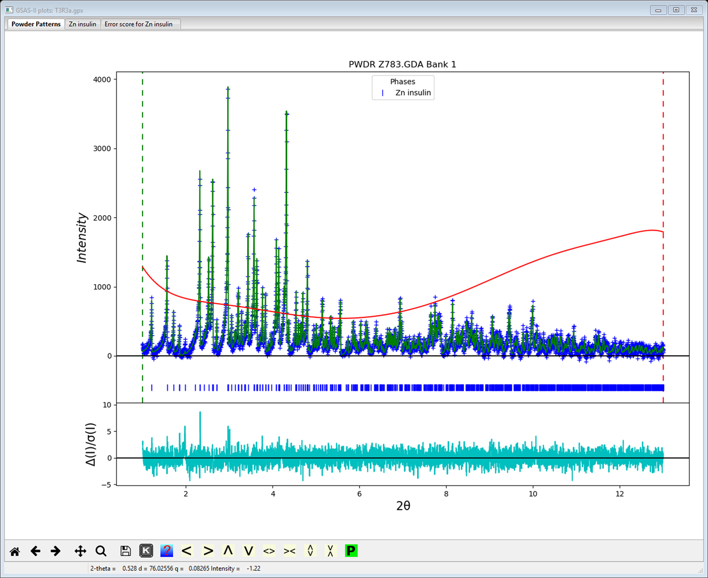
Figure 2. Refinement fit using GSAS-II for T3R3f Zn-insulin variant powder data reported by Von Dreele, et al. (Reference Von Dreele, Stephens, Blessing and Smith2000). Observed data (blue+) and calculated profile (green line) (minus background) are shown. Red curve is the fitted background profile. The weighted difference curve is at bottom.

Figure 3. Protein structure validation via Errat (“Error score 1”) and Errat2 (“Error score 2”) routines (Colovos and Yeates, Reference Colovos and Yeates1993) as implemented in GSAS-II. Horizontal dashed lines indicate 90 and 95% confidence levels for invalid residue structures. Those residues likely to be in error are shown in red.
V. CONCLUSION
The combination of using flexible rigid bodies to represent the amino acid residues in a protein structure and implementing a Levenberg–Marquardt least squares provides a well-behaved refinement approach to protein structures and powder diffraction data. The inclusion of a SVD for the required matrix inversion provides a means of dealing with the inherently under determination of these problems.
Acknowledgement
Use of the Advanced Photon Source, an Office of Science User Facility operated for the US Department of Energy (DOE) Office of Science by Argonne National Laboratory, and this work was supported by the US DOE under Contract no. DE-AC02-06CH11357.


