


INTRODUCTION
The timing and green-up of vegetation are key ecosystem responses that reflect climate–vegetation functioning, and have become emerging indicators of global environmental changes (Clark et al. Reference CLARK, CARPENTER, BARBER, COLLINS, DOBSON, FOLEY, LODGE, PASCUAL, PIELKE, PIZER, PRINGLE, REID, ROSE, SALA, SCHLESINGER, WALL and WEAR2001). Leaf phenology is strongly related to temperature in middle and high latitudes climates, and to rainfall in seasonally dry climates (Zhang et al. Reference ZHANG, FRIEDL and SCHAAF2006). A recent study in the Amazon has shown that the southern equatorial regions have a distinctive canopy phenology with net leaf flush being responsive to seasonality in solar irradiance, and also to variation in dry-season length (Jones et al. Reference JONES, KIMBALL and NEMANI2014). Therefore, leaf phenology might be expected to be one of the most easily observable ecosystem functions that change in response to climate.
Relationships between phenological variation with climate (van Leeuwen et al. Reference VAN LEEUWEN, DAVISON, CASADY and MARCH2010, Zhang et al. Reference ZHANG, FRIEDL, SCHAAF, STRAHLER and LIU2005) and vegetation communities (Davison et al. Reference DAVISON, BRESHEARS, VAN LEEUWEN and CASADY2010) can be analysed through remote-sensing analysis. Recent studies have suggested differences in phenological patterns of vegetation in relation to land-use change in temperate and tropical regions (de Beurs & Henebry Reference DE BEURS and HENEBRY2004, Suepa et al. Reference SUEPA, QI, LAWAWIROJWONG and MESSINA2016), and in response to timber extraction in the Amazon forests (Koltunov et al. Reference KOLTUNOV, USTIN, ASNER and FUNG2009). Across subtropical regions, phenological variation and particularly the effects of climate and disturbance on canopy leaf phenology remains largely understudied. However, subtropical forests may have large impacts on the global carbon cycle (Zhang et al. Reference ZHANG, CRISTIANO, ZHANG, CAMPANELLO, TAN, ZHANG, CAO, GOLDSTEIN, Goldstein and Santiago2016). A better understanding of phenological drivers is necessary to predict potential impacts of climate change and forest use on carbon balance in subtropical regions.
Subtropical forests in South America include dry forests, seasonally deciduous forests, cloud evergreen–semi-deciduous forests and moist semi-deciduous forests. Seasonal forests in north-western Argentina have experienced an increase in rainfall during the past decades (Ferrero & Villalba Reference FERRERO and VILLALBA2009). At the same time, a pronounced decrease in rainy days with changes in rainfall distribution patterns is expected in moist semi-deciduous forests in the north-east (Pizarro et al. Reference PIZARRO, MEZHER, MERCURI and ESPÍNDOLA2013), which are also experiencing an increment in mean temperatures (Salazar et al. Reference SALAZAR, NOBRE and OYAMA2007). In addition, extensive areas are affected by extensive cattle ranching, selective logging and firewood extraction, with negative effects on the forest structure, particularly a reduction in tree above-ground biomass, and changes in species composition and ecosystem functioning (Blundo & Malizia Reference BLUNDO, MALIZIA, Brown, Blendinger, Lomáscolo and García Bes2009, Campanello et al. Reference CAMPANELLO, GATTI, ARES, MONTTI and GOLDSTEIN2007).
In this study, we analysed remote-sensing data to describe phenological patterns in combination with field data from 131 permanent plots established in old-growth and disturbed forests to carry out a comprehensive regional analysis of leaf phenological patterns and their relationships with climate and forest-use along subtropical forests of South America. In particular, we assessed how rainfall and temperature are related to leaf phenological patterns across a subtropical environmental gradient, and analysed how changes in forest structural characteristics, such as stock of above-ground biomass, as a consequence of human activity relate to the observed phenological signals across the gradient. We tested the following hypotheses: (1) tree phenology will respond to rainfall in subtropical seasonal forests (Malizia et al. Reference MALIZIA, PACHECO, BLUNDO and BROWN2012, Suepa et al. Reference SUEPA, QI, LAWAWIROJWONG and MESSINA2016), while in humid subtropical forests leaf flushing will be associated with daylight and temperature (di Francescantonio Reference DI FRANCESCANTONIO2017, Marques et al. Reference MARQUES, ROPER and BAGGIO SALVALAGGIO2004), and (2) changes in the stock of above-ground biomass and in the distribution of species traits, in particular, leaf phenology and wood density, will affect the phenological signal in disturbed forests.
METHODS
Study area and forest types
In South America, Atlantic forest, Chaco and Andean forest are forest types distributed from tropical areas that reach their southern limit in North Argentina. In this part of their distribution, climate is defined as subtropical because temperatures may drop considerably generating occasional frost during the cold months (Brown et al. Reference BROWN, GRAU, MALIZIA, GRAU, Kappelle and Brown2001). The study area includes these three forest types which involve forests with different phenological patterns, distributed within an area of about 150000 km2 (22–28°S, 54–65°W). These forests cover a wide range of altitude (from 200 m to c. 3000 m asl), rainfall (from 400 to more than 2000 mm y−1) and mean annual temperatures (from 14 to 24°C). Most of these forests experience some degree of human intervention such as extensive cattle ranching, selective logging and firewood extraction.
The Andean forest extends along an altitudinal gradient from 400 to 3000 m asl, and represents the southernmost extension of Neotropical montane forests located on the eastern Andean slope (Cabrera & Willink Reference CABRERA and WILLINK1980). We considered three vegetation units based on traditional floristic classification (Brown Reference BROWN, Churchill, Balslev, Forero and Luteyn1995): premontane forest (PF) from c. 400–900 m asl, low montane forest (LMF) from c. 900–1600 m asl, and high montane forest (HMF) from c. 1600–3000 m asl. Premontane forests are seasonal dry forests with >80% deciduous tree species (Sarmiento Reference SARMIENTO1972). Low and high montane forests are cloud forests with a high proportion of evergreen and semi-deciduous tree species (Brown et al. Reference BROWN, GRAU, MALIZIA, GRAU, Kappelle and Brown2001). Rainfall is concentrated from November to March with mean values of 820 mm y−1 (550–1400 mm y−1) in PF, 1800 mm y−1 (1100–2300 mm y−1) in LMF, and 1100 mm y−1 (800–1400 mm y−1) in HMF (Bianchi & Yáñez Reference BIANCHI and YÁÑEZ1992). In cloud forests, water input through fog interception can equal direct rainfall (Hunzinger Reference HUNZINGER1997). Mean annual temperature decreases along the altitudinal range from 21.5°C to 11.7°C (Arias & Bianchi Reference ARIAS and BIANCHI1996).
The dry Chaco forest (DCF) covers a significant area of Bolivia, Paraguay and Argentina. It is a seasonal dry forest with vegetation dominated by broad-leaved, deciduous or semi-deciduous trees, with temperate floristic affinities (Pennington et al. Reference PENNINGTON, LAVIN and OLIVEIRA-FILHO2009). A sub-humid monsoonal rainfall pattern (400–900 mm y−1) and very high absolute temperatures (48°C) create a marked water deficit in this forest type (Prado Reference PRADO1993), mainly from September to November.
The Atlantic forest includes from semi-deciduous to evergreen forests distributed along 3300 km of the Atlantic coast of Brazil, south-eastern Paraguay and north-eastern Argentina (Galindo-Leal & Gusmão Câmara Reference GALINDO-LEAL, GUSMÃO CÂMARA, Galindo-Leal and Gusmão Câmara2003). Nearly 11000 km2 of semi-deciduous Atlantic forests (SAF) remains in the north-eastern corner of Argentina and represents the largest remnant of continuous semi-deciduous Atlantic Forest. This semi-deciduous forest contains deciduous, brevi-deciduous and evergreen tree species, with deciduous accounting for 25–50% of the tree species (Leite & Klein Reference LEITE and KLEIN1990). Many of the species are also present in seasonally dry forests in South America (Pennington et al. Reference PENNINGTON, LAVIN and OLIVEIRA-FILHO2009, Werneck et al. Reference WERNECK, COSTA, COLLI, PRADO and SITES2011). Mean annual precipitation in this area is about 2000 mm y−1 evenly distributed but with unpredictable dry spells occurring throughout the year. Mean annual temperature is 21°C with monthly means of 25°C in warmest month (January), and 15°C in coldest month (July). Frost seldom occurs in colder months.
Field sampling
We used data from 131 permanent plots (Figure 1). Plots were established in old-growth forests and disturbed forests, which have had some degree of human intervention in the last decades. In Andean forests, the traditional forest-uses were extensive cattle ranching and selective logging, but their intensity changes along the altitudinal gradient. In DCF, cattle ranching and selective logging were also the principal uses, in addition to firewood extraction from local communities. The predominant use in the SAF was selective logging and plots inside protected areas did not have human intervention in the last 70 y. Difference in above-ground biomass between plots in old-growth forest and plots in disturbed forest were significant for all forest types except HMF (Appendix 1).
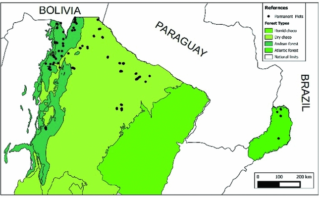
Figure 1. Location of 131 permanent plots across forest types in north Argentina.
In each permanent plot all living woody stems (such as trees, palms and ferns) ≥10 cm of diameter at breast height (dbh) were measured and identified to species. In Andean forests, 20 1-ha plots were established in PF, 16 1-ha plots and one 6-ha plot in LMF, and 14 1-ha plots and 10 0.24-ha plots in HMF, all distributed between 22–27°S and measured between 2002 and 2008. The form of plots was square (100 × 100 m) or rectangular (20 × 500 m or 40 × 60 m). Regardless of the plot size, all trees with >10 cm dbh were marked with numbered aluminium tags, measured for dbh (1.30 m height, avoiding trunk irregularities) and identified to species or morphospecies level in every plot. In DCF, the sample unit was a 100 × 100-m cluster with a set of circular concentric plots placed at each vertex (Gasparri & Baldi Reference GASPARRI and BALDI2013). In one of these plots (with an area of 500 m2 and a radius of 12.6 m) all trees with a dbh >10 cm were recorded; in other plots (area of 1000 m2 and radius of 17.8 m), trees with dbh >20 cm were recorded. In summary, 50 plots that represent a surveyed area of 20 ha were established during 2007. In SAF, 20 1-ha permanent plots of 100 × 100 m were established between 2000 and 2003, in which all living stems ≥10 cm dbh were recorded and marked, with the exception of lianas.
Above-ground biomass estimation and climatic data
For each plot we estimated above-ground biomass using equations developed by Chave et al. (Reference CHAVE, ANDALO, BROWN, CAIRNS, CHAMBERS, EAMUS, FÖLSTER, FROMARD, HIGUCHI, KIRA, LESCURE, NELSON, OGAWA, PUIG, RIERA and YAMAKURA2005) for humid and dry forests. We obtained wood density for each species using local databases (Easdale et al. Reference EASDALE, HEALEY, GRAU and MALIZIA2007, http://www.inti.gov.ar/), or an international database when local data were unavailable (Chave et al. Reference CHAVE, MULLER-LANDAU, BAKER, EASDALE, TER STEEGE and WEBB2006). If published data of wood density did not exist for a particular species we used the following criteria: (1) we used the wood density information from the species of the same genera growing in the closest geographic location (e.g. to estimate the biomass of Solanum grossum we used the wood density of Solanum riparium); (2) alternatively, we used the wood density data for the genus reported in Chave et al. (Reference CHAVE, MULLER-LANDAU, BAKER, EASDALE, TER STEEGE and WEBB2006), and (3) if this was not possible we used the data reported for the family. If the tree individual was unidentified to species level but we knew either the genus or family (12% of total individuals measured) we also used the wood density data from Chave et al. (Reference CHAVE, MULLER-LANDAU, BAKER, EASDALE, TER STEEGE and WEBB2006). Finally, if the individual was unidentified to any taxonomic level (0.4% of total individuals measured) we used the average value of wood density of the plot where that particular tree occurred. In order to estimate above-ground biomass for palms and ferns we used the equation developed by Frangi & Lugo (Reference FRANGI and LUGO1985) and Weaver (Reference WEAVER2000), respectively. The biomass distribution pattern showed that Atlantic and Andean forests presented highest above-ground biomass per plot than dry Chaco forests (F = 49.2; P < 0.0001) (Figure 2a). The phenological classification of species in deciduous, semi-deciduous and evergreen species was made with literature data (Custódio Talora & Morellato Reference CUSTÓDIO TALORA and MORELLATO2000, Legname Reference LEGNAME1982, Lima Pilon et al. Reference LIMA PILON, GIASSI UDULUTSCH and DURIGAN2015, Martín et al. Reference MARTÍN, NICOSIA and LAGOMARSINO1997) and observational data.
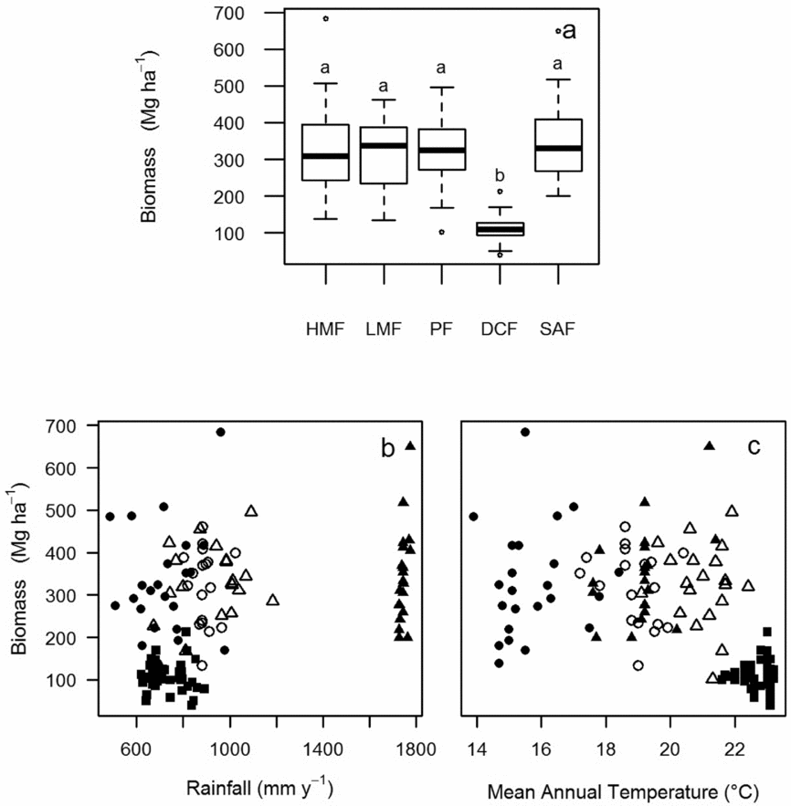
Figure 2. Boxplot of biomass against forest types (a). Lowercase letters indicate significant differences among forest types. Forest types are ordered according to the geographic gradient from west to east: high montane forest (HMF); low montane forest (LMF); premontane forests (PF); dry Chaco forest (DCF); and semi-deciduous Atlantic forest (SAF). Scatterplots of biomass against total annual rainfall (b) and mean annual temperature (c). Symbols represent plots located in HMF (black circles); LMF (white circles); PF (white triangles); DCF (black squares); and SAF (black triangles).
We obtained climatic data (mean annual temperature and rainfall) from the global database WorldClim for each permanent plot (Hijmans et al. Reference HIJMANS, CAMERON, PARRA, JONES and JARVIS2005). Because of high collinearity among explanatory variables (i.e. biomass and climatic factors) can lead to relationships that are difficult to interpret when using multiple regression models, low correlations among explanatory variables are desirable. In our study, biomass correlated negatively with temperature (r = 0.57; P < 0.0001) and positively with rainfall (r = 0.39; P < 0.0001), which can be considered moderate correlation values, which need to be addressed in interpreting the results but do not invalidate them. In DCF, where the mean annual temperature is higher in combination with low levels of rainfall, the relationship between biomass and climatic factors showed less variation among plots in comparison to the moister forest types (Figure 2b, c).
Remote-sensing data and phenological metrics
MODIS images from 16-day composite time-series at 250-m resolution were used to derive land-surface phenological metrics from Enhanced Vegetation Index (EVI). We used the TIMESAT program (Jönsson & Eklundh Reference JÖNSSON and EKLUNDH2004) to process EVI data from Julian day 289 year 2000, to Julian day 273 year 2008 (23 points y−1 × 8 y = 184 points). TIMESAT fits local functions to the time-series data points, and then combines these functions into a global model. Phenological metrics for each growing season are then extracted from the smoothed function, thereby reducing the influence of signal noise in the raw data. The temporal window does not align with calendar years, but allows the program to have ample data to fit a full function to the main southern hemisphere growing seasons from 2001–2002 to 2007–2008. A custom program was created to obtain several phenological metrics calculated for each growing season (e.g. season amplitude, peak and base value) as raster bands in a stack for each calendar year. Each image pixel was processed independently and phenological metrics were labelled with the year in which the season started. Finally, we extracted the phenological metrics for the pixel corresponding to the location of each of the 131 permanent plots. Although pixels cover a larger area than plots, we assumed that plots are representative of the surrounding vegetation (e.g. no plots were established near transformed areas). The data extracted correspond to the year of the survey of each plot, except for the case of the Atlantic forest, where the plot surveys correspond to the year 2000 and the satellite data to the year 2001.
We used nine phenological metrics from TIMESAT in our analysis: (1) season start, and (2) season length, to compare timing of vegetation growth measured in days; (3) peak value, (4) base value, (5) small integral, (6) large integral, (7) season amplitude, to account for the magnitude of EVI values; and (8) left derivative and (9) right derivative, which are related to the velocity of growth at the beginning and ending of the season growth, respectively (Figure 3). An additional variable was the coefficient between the small and large integrals that we calculated to obtain the proportion of biomass produced in the growing season. The small integral describes the vegetation production in the growth season. And the large integral, an integration of all fitted EVI values over the season, is a measure that has been related to net ecosystem production (Prince & Goward Reference PRINCE and GOWARD1995).
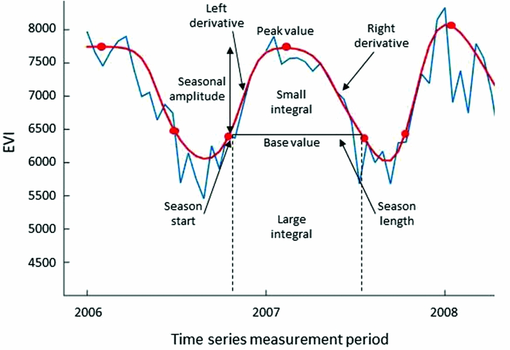
Figure 3. Nine phenological metrics derived from Enhanced Vegetation Index (EVI) time-series data using TIMESAT over 1 y of growth in a randomly selected permanent plot. Blue curve represents real data, and red curve represents fitted model function.
Data analysis
We performed a principal component analysis (PCA) to synthesize the phenological metrics in ecophysiological patterns related to productivity, seasonality and phenology (as was previously described in Davison et al. Reference DAVISON, BRESHEARS, VAN LEEUWEN and CASADY2010), and to identify phenological groups to complement our a priori classification of plots in five forest types (i.e. HMF, LMF, PF, DCF and SAF). We used the broken-stick method to identify interpretable ordination axes (Jackson Reference JACKSON1993). We used analysis of variance and Tukey test to describe the regional variation in the phenological patterns (i.e. significant and interpretable PC axes) among forest types. We performed multiple regression models to assess the relative importance of rainfall, temperature and biomass to explain phenological patterns across subtropical forests and within forest types. The relative importance refers to the quantification of a predictor variable's contribution to a multiple regression model. Johnson & Lebreton (Reference JOHNSON and LEBRETON2004) defined relative importance as the proportionate contribution that each predictor makes to R2, considering both its direct effects and its effect when combined with the other variables in the regression equation. We used the lmg metric (Lindeman et al. Reference LINDEMAN, MERENDA and GOLD1980) to decompose R2 into non-negative contributions that automatically sum to the total R2. The approach taken by the lmg metric is based on sequential R2, but takes care of the dependence on orderings by averaging over orderings, using simple unweighted averages (Grömping Reference GRÖMPING2006). Furthermore, to evaluate variation in forest structure and species composition among plots within each forest type, we performed non-metric multidimensional scaling (NMDS) to correlate plot-scores with biomass, and species-scores with leaf phenology (deciduous, semi-deciduous and evergreen) and wood density. We used R program (http://www.R-project.org/), in particular, we used relaimpo package (Grömping Reference GRÖMPING2006) to assess relative contribution of each explanatory variable and BiodiversityR package (Kindt & Coe Reference KINDT and COE2005) to multivariate analysis.
RESULTS
Phenological patterns in subtropical forests
The ordination of the 131 plots across the phenological multidimensional space based on 10 phenological metrics was congruent with the traditional biogeographic classification, differentiating the samples from the five forest types; although the differentiation between LMF and PF of the Andean forests was less clear (Figure 4). The first three PC axes were significant and explained 85% of the variation in the phenological metrics across subtropical forests sorting out plots along indicators of seasonality, productivity and phenology. The first interpretable PC (PC 1, 40%) was negatively related to seasonal amplitude, left derivative, small integral and peak value (Table 1) and distributed plots along a forest seasonality gradient. Plots with lowest scores on PC 1 showed higher values of seasonal amplitude (i.e. higher changes in EVI between dormancy and growth season), higher small integral, and higher left derivative (i.e. higher velocity of growth at the beginning of the season growth). These plots were located in Andean forests indicating that they represent the most seasonal forests (Figure 4). In addition, PC 1 was correlated positively with temperature and negatively with the biomass per plot (Table 1) showing that plots with positive scores on PC 1 (i.e. DCF) exhibited higher values of temperature and low biomass per plot. The second interpretable PC (PC 2, 26%) was positively related to base value and large integral, and negatively related to the coefficient between integrals. Higher base and large integral values indicate that plots located in the positive scores of PC 2 present higher above-ground biomass productivity. In accordance, rainfall and biomass were correlated positively with PC 2 (Table 1) increasing toward plots located in SAF. Finally, the third PC (PC 3, 19%) was positively related to season length, and negatively related to season start showing a more gradual distribution along phenological indicators mainly related to time measures. Right derivative that represents the velocity of growth in the season-end was also related with PC 3.

Figure 4. Principal components (PC) ordinations of 131 plots based on 10 phenological metrics. Symbols represent plots located in high montane forest (black circles); low montane forest (white circles); premontane forest (white triangles); dry Chaco forest (black squares); and semi-deciduous Atlantic forest (black triangles).
Table 1. Percentage of variance explained by the principal components analysis of 131 plots established in subtropical forests of Argentina; loadings of 10 phenological metrics on the first three significant components and Spearman Rank correlations among explanatory variables with phenological metrics and PC axes. Coefficients of correlation with P < 0.001 are showed. MAT = Mean Annual Temperature.

Regional variation in seasonality and productivity (i.e. PC 1 and PC 2, respectively) differed among forest types (F = 62.3; P < 0.0001, and F = 60.6; P < 0.0001, respectively), but variation in phenology did not (PC 3, F = 2.06; P = 0.09). Although DCF and SAF were different in terms of indicators of productivity, they were the least seasonal forests given their low seasonal amplitude, left derivative and small integral relative to HMF, LMF and PF; the Andean forest types did not differ significantly in indicators of seasonality (Figure 5a–c). The SAF followed by LMF and PF showed the highest indicators of productivity consistent with high base value and high large integral (i.e. high annual GPP). Finally, although there was no significant difference in PC 3 scores among forest types, plots located in DCF (mainly) and in PF tended to show higher season length (Figure 5h).

Figure 5. Boxplots of phenological metrics (EVI values) against forest types: (a–d) metrics related to forests seasonality, i.e. PC 1; (e–g) metrics related to forests productivity, i.e. PC 2; and (h–j) metrics related to forests phenology, i.e. PC 3. HMF = high montane forest; LMF = low montane forest; PF = premontane forests; DCF = dry Chaco forest; SAF = semi-deciduous Atlantic forest.
Relationships among phenological patterns, climate and biomass
Climate showed the highest relative importance to explain variation in seasonality and productivity patterns across subtropical forests. Temperature showed higher relative importance on seasonality pattern (27%), and rainfall showed higher relative importance on productivity pattern (47%). In addition, variation in forest biomass showed about 15% of relative importance to explain seasonality and productivity patterns across the regional gradient (Table 2).
Table 2. Relative importance (and slope sign) estimated with the lmg metric (Lindeman et al. Reference LINDEMAN, MERENDA and GOLD1980) for each explanatory variable in multiple regression models for seasonality (PC 1), productivity (PC 2), and phenology (PC 3) patterns. Models fitted for all forests of subtropical gradient and for each forest type: HMF = high montane forest, LMF = low montane forest, PF = premontane forests, DCF = dry Chaco forest, SAF = semi-deciduous Atlantic forest. MAT = mean annual temperature.

When each forest type was analysed separately, the proportion of total variance explained, and the relative importance of each explanatory variable were different for forest seasonality, productivity and phenology. Seasonality was significantly explained only in cloud forests (i.e. HMF and LMF). Climate showed higher relative importance to explain seasonality, however rainfall was higher in HMF (32%) and temperature was higher in LMF (25%). Biomass showed 12% of relative importance to explain the seasonality pattern in HMF while only 4% in LMF, both with positive slopes (Table 2), i.e. plots with higher seasonal amplitude and higher left derivative (lowest scores on PC 1) tended to show higher biomass per plot. Species composition in cloud forests differed among plots as shown in the ordination analysis (Figure 6a, b), but only in HMF was there a relationship between biomass and variation in species composition along axis 1 (Appendix 2). In HMF plots with negative scores on NMDS 1 had high biomass and showed high abundance of evergreen tree species (Figure 6a).
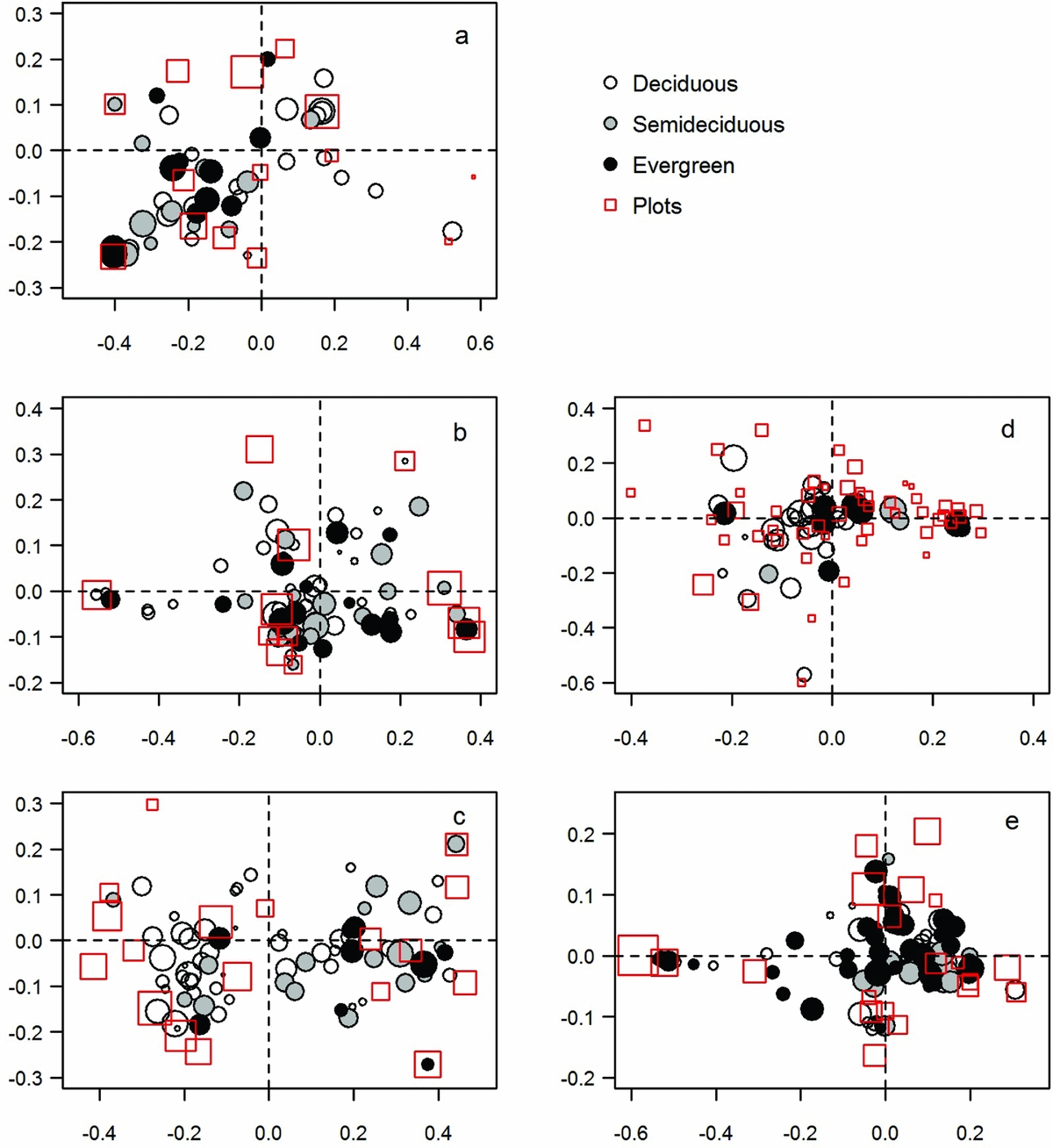
Figure 6. Species and plots NMDS ordinations for each forest type. High montane forest (a); low montane forest (b); premontane forests (c); dry Chaco forest (d); semi-deciduous Atlantic forest (e). Circles size (species) control by woody density and squares size (plots) control by biomass.
The productivity pattern was explained mainly by climate within Andean forests (Table 2), with temperature showing the highest relative importance (~40%) in cloud forests whereas rainfall had the highest relative importance in PF (45%). That is, within cloud forests, plots with higher mean annual temperature tend to shown higher base value and large integral, while within PF these phenological metrics increased in plots with higher annual rainfall. Only in PF did biomass show a relative importance of about 8% to explain phenological variation related to indicators of productivity (Table 2). Species composition differed in PF and this variation was correlated with biomass and foliar phenology of trees. Species scores of NMDS 1 were positively correlated with leaf phenology of tree species (r = 0.41; P < 0.001), and plot scores of axis 2 were negatively correlated with biomass (r = −0.57; P < 0.01, Appendix 2). That is, plots with negative scores on NMDS 1 and NMDS 2 tended to present high biomass and showed high abundance of deciduous tree species (Figure 6c).
The third PC axis mainly related to time measures (i.e. season length and season start, both measures in days) was explained only within DCF (R2 = 0.24; P < 0.01) by biomass and rainfall (11% and 9% of relative importance, respectively). Although species scores were correlated with NMDS 1 showing higher abundance of evergreen species on the positive side of this axis (Figure 6d), this variation in species composition was not related with biomass at the plot level (Appendix 2). Finally, no phenological patterns were explained either by climate or biomass in SAF (Table 2). However, plots score of NMDS 1 and NMDS 2 were correlated with biomass (r = −0.48 and r = 0.47, respectively; P < 0.05) and species scores were correlated with wood density (r = −0.40; P < 0.001) showing variation in forest structure and species composition in this forest type (Figure 6e, Appendix 2).
DISCUSSION
Phenological patterns across subtropical forests
Our combined analyses of field and remote-sensing data allowed us to distinguish two principal phenological patterns across the region. On one hand, Andean forests are the most seasonal forests as indicate their higher values of seasonal amplitude. This phenological metric represents the change in EVI values between dormancy and seasonal growth over the year (Paruelo & Lauenroth Reference PARUELO and LAUENROTH1995). Subtropical Andean forests have a marked dry season which matches with colder temperatures, representing the dormancy stage. After dormancy, they start an accelerated growth during the rainy season with temperatures that may exceed 40°C in the lowlands; these wet and warmer conditions occur for 4–5 mo y−1 (Brown et al. Reference BROWN, GRAU, MALIZIA, GRAU, Kappelle and Brown2001, Kessler & Beck Reference KESSLER, BECK, Kappelle and Brown2001). In contrast, Atlantic forest shows a precipitation pattern more evenly distributed over the year without dry season (Crespo Reference CRESPO1982), and dry Chaco forest tends to present warmer conditions along the year. These climatic conditions without a marked dry/wet or cold/warm season in Atlantic and Chaco forests would promote lower changes in the photosynthetic activity between dormancy and growth, and consequently less change in EVI relative to Andean forests.
On the other hand, the productivity pattern in subtropical forests described along axis 2 of PCA is supported by the base value and the large integral. The large integral is a measure that has been related to net primary production (NPP) and net ecosystem production (Prince & Goward Reference PRINCE and GOWARD1995). The large integral and the base value are greater in semi-deciduous Atlantic forest indicating that these forests present the higher aboveground biomass production. In diverse forest ecosystems, greater leaf area index can lead to higher NPP in both dormant and growing seasons (Knapp et al. Reference KNAPP, BRIGGS, COLLINS, ARCHER, BRET-HARTE, EWERKS, PETERS, YOUNG, SHAVER, PENDALL and CLEARLY2008). The semi-deciduous Atlantic forest has a high diversity of evergreen and semi-deciduous tree species that maintain continuous growth, and has also high potential canopy photosynthesis throughout the year (Cristiano et al. Reference CRISTIANO, MADANES, CAMPANELLO, DI FRANCESCANTONIO, RODRIGUEZ, ZHANG, OLIVA CARRASCO and GOLDSTEIN2014). In this study, semi-deciduous Atlantic forest had the highest productivity (as indicated by base value and large integral, Figure 5e, f), with the coefficient between small and large integrals being significantly lower (i.e. the proportion of biomass produced strictly in the growing season, which is the time of the year with highest values of EVI) in comparison to other forests (Figure 5g). Indeed, only about 24% of the biomass in the Atlantic forest is produced in the growing season. The low seasonality in their climatic conditions (e.g. rainfall regularly distributed) tends to promote a relatively high biomass production throughout the year in comparison with other productive but more seasonal forests like LMF and PF. Our results show that in these two seasonal forests (i.e. LMF and PF), about 40% of the biomass is produced in the rainy season (i.e. around 4 mo in the year). At the other extreme, DCF seems to have a low but constant rate of biomass production over a longer growth season promoted by relatively warmer conditions throughout the year (Gasparri & Baldi Reference GASPARRI and BALDI2013). This dry forest also produces about 40% of its biomass in the growing season (i.e. the time of the year with highest values of EVI) as reflected by the small/large integral coefficient (Figure 5g).
Satellite-derived patterns of phenology clearly reflect differences among forest types traditionally defined on the basis of floristic composition and physiognomy. This implies that within forest types there may be common ecophysiological controls, potentially relevant for management and conservation of functional diversity, and ecological processes such as carbon storage and water availability. Phenological metrics has been proving useful to classify biomes in other studies (Wessels et al. Reference WESSELS, STEENKAMP, VON MALTITZ and ARCHIBALD2011). Indicators of seasonality and productivity, such as seasonal amplitude and base value, respectively, could be used to map and classify forest types through remote sensing in the subtropical gradient studied.
Influence of climate and biomass on phenological patterns
We found that seasonality and productivity patterns are explained mainly by regional climatic variation and to a lesser extent by biomass; changes in the stock of biomass and the species composition in disturbed forests affect phenological signal measured through EVI metrics. Mean annual temperature explained about 30% of forest seasonality, and annual precipitation explained about 50% of forest productivity. Many studies have reported associations between phenological metrics and regional climate (Brando et al. Reference BRANDO, GOETZ, BACCINI, NEPSTAD, BECK and CHRISTMAN2010, Linderman et al. Reference LINDERMAN, ROWHANI, BENZ, SERNEELS and LAMBIN2005, van Leeuwen et al. Reference VAN LEEUWEN, DAVISON, CASADY and MARCH2010) indicating that EVI (or NDVI) capture spatial patterns in photosynthetic responses of vegetation to regional gradients of temperature and rainfall. In general, our results are congruent with these studies, in which changes in phenological metrics between dormancy and growing season (i.e. seasonality) are influenced by temperature, and the magnitude of these changes (i.e. productivity) is influenced by rainfall.
When biomass is taken into account as measure of forest structure, it adds explanatory power in the variation of phenological patterns, explaining about 15% of forest seasonality and productivity across the regional gradient (Table 2). Plant cover may represent an ecological dimension that complements phenology, seasonality and productivity in understanding landscape-scale patterns and forests dynamics (Davison et al. Reference DAVISON, BRESHEARS, VAN LEEUWEN and CASADY2010). Within forest type, climate remains relatively constant, so differences in biomass between old-growth and disturbed forest could increase the relative importance of biomass to explaining phenological patterns. In some of the forest types studied, we found that changes in forest structure and species composition in disturbed forests affect phenological metrics such as seasonal amplitude (indicator of seasonality) and base value (indicator of productivity).
We found that forest biomass contributed to explain a proportion of phenological variation within HMF, PF and DCF. In HMF, plots differ in species composition and this variation is correlated with the stock of biomass per plot. Although above-ground biomass did not differ significantly between old-growth and disturbed forests (Appendix 1), plots with higher biomass tend to have higher abundance of evergreen species, most of them belonging to the Myrtaceae, which have high wood density (e.g. Blepharocalyx salicifolius, Myrcianthes mato, M. pseudomato). In this forest type, cattle ranching is an historical anthropogenic disturbance that has been practiced by local communities in Andean forests for at least the past 100 y (Brown et al. Reference BROWN, GRAU, MALIZIA, GRAU, Kappelle and Brown2001), and is a determinant of species composition at the landscape scale (Blundo et al. Reference BLUNDO, MALIZIA, BROWN and BLAKE2012). Cattle ranching does not seem to reduce above-ground biomass but may affect species composition after decades of forest-use. Biomass also affects phenological metrics of forest productivity in premontane forest. Within PF, plots with higher biomass have higher abundance of deciduous species with high wood density. In PF, old-growth forests are dominated by Anadenanthera colubrina, Phyllostylon rhamnoides and Calycophyllum multiflorum, all timber species with high wood density. Biomass is significantly lower in forests disturbed by selective logging in recent decades (F = 10.1; P < 0.01; N = 20), not only because logging decreases tree density and large trees are scarce but also because species with low wood density are promoted after timber extraction (e.g. Ocotea puberula, Chrysophyllum gonocarpum). In premontane forest, biomass distribution varies according to climate at a regional spatial scale and to selective logging history at the landscape scale (Blundo et al. Reference BLUNDO, MALIZIA and GONZÁLEZ-ESPINOSA2015). Finally, variation in forest biomass may affect the phenological timing in DCF (Table 2), i.e. phenological metrics such as season length and start day. Within Chaco forest, areas of sparse vegetation frequently alternate with dense forested areas dominated by two or three tree species, or forested areas dominated by shrubs and cacti (Cabrera Reference CABRERA1976, Giménez & Moglia Reference GIMENEZ and MOGLIA2003). In addition, a rainfall gradient decreases from both margins to the centre of this forest type, with mean annual rainfall of 900 mm (at the west and east sides) to 400 mm toward the centre (Minetti Reference MINETTI1999). These gradients of forest structure and humidity tend to influence the phenology of DCF, mainly the length and the start-day of the growing season. Stands with high biomass are able to maintain high photosynthetic activity at the end of the growing season (Gasparri et al. Reference GASPARRI, PARMUCHI, BONO, KARSZENBAUM and MONTENEGRO2010). These forests are dominated by large trees of hard-wooded evergreen species (e.g. Aspidosperma quebracho-blanco, Schinopsis lorentzii and Ziziphus mistol), that are able to exploit deep water and thus have a relatively longer growing season. In contrast, low-biomass plots that result from the removal of large trees and cattle grazing develop a canopy of small trees and shrubs that rely mostly on surface water and rainfall pulses (Gasparri & Baldi Reference GASPARRI and BALDI2013, Gasparri et al. Reference GASPARRI, PARMUCHI, BONO, KARSZENBAUM and MONTENEGRO2010), thus having a shorter season length and later growth start. We suggest that increasing the proportion of plots with changes in forest structure due to recent forest-use will probably increase the relative importance of biomass, or another parameter of structure, to explain phenology within forest types. In this way, identifying key phenological metrics, such as the base value or the peak value (both highly correlated with biomass as shown in Table 1), may be an additional tool for monitoring changes in forest structure related to different forest-use practices across large geographic areas.
There were no relationships between the phenological dynamic and climate or biomass in the semi-deciduous Atlantic forest. The plots studied differed in biomass due mostly to selective logging, but also to species composition changes. Plots with higher biomass were found in warmer areas and were dominated by an evergreen species with relatively high value of wood density (Aspidosperma polyneuron) and the tropical palm Euterpe edulis. Selective logging causes liana and evergreen bamboo encroachment (Campanello et al. Reference CAMPANELLO, GATTI, ARES, MONTTI and GOLDSTEIN2007), which is likely to mask any phenological signal from trees in remote-sensing studies (Cristiano et al. Reference CRISTIANO, MADANES, CAMPANELLO, DI FRANCESCANTONIO, RODRIGUEZ, ZHANG, OLIVA CARRASCO and GOLDSTEIN2014). Davison et al. (Reference DAVISON, BRESHEARS, VAN LEEUWEN and CASADY2010) found that communities with high species diversity present poor or null relationships between NDVI dynamics and plant cover. These authors suggest that communities with high species diversity might have mixed signals for vegetation seasonality, phenology and productivity that could outweigh general influences of biomass and climate on these patterns. Consistently, the semi-deciduous Atlantic forest has the highest biodiversity of all subtropical forests studied, and is included among the 25 top biodiversity hotspots in the world (Myers et al. Reference MYERS, MITTERMEIER, MITTERMEIER, DA FONSECA and KENT2000). Many tree species in the SAF are shared with seasonally dry tropical forests while other have an Amazonian lineage or link to the Atlantic moist forests (Pennington et al. Reference PENNINGTON, LAVIN and OLIVEIRA-FILHO2009). The confluence of different phytogeographic domains in this region may contribute to the absence of patterns among the variables studied. A different approach is necessary to accurately predict changes in forest structure and function from remote-sensing analysis in these forests.
In summary, the type of forest use may affect ecosystem functioning through changes in forest structure and species composition in subtropical forests. For example, we found that plots established in old-growth forests of Andean cloud forests have higher above-ground biomass and higher abundance of evergreen tree species in comparison to plots established in disturbed forests with low biomass and higher abundance of deciduous tree species. These changes in forest structure affect phenological signals such as seasonal amplitude or base value, and consequently change leaf phenological patterns in disturbed forest stands. Considering forest biomass in the analysis of the seasonal patterns and trends of EVI dynamics should help to differentiate year-to-year variability from global change effects, e.g. die-off or land-cover changes (Bradley & Mustard Reference BRADLEY and MUSTARD2008). Finally, changes in annual precipitation or mean annual temperature as predicted to the study area, or an increase in the forest-use pressure without proper forest management practices can lead to changes in leaf phenological patterns across South American subtropical forests.
ACKNOWLEDGEMENTS
This study was funded by a postdoctoral grant from CONICET to C. Blundo. We thank two anonymous reviewers for their comments.
Appendix 1. Mean (and range in parentheses) values of rainfall (mm y−1), mean annual temperature (MAT; °C) and biomass (Mg biomass ha−1) for each forest type. Number of plots and biomass are discriminated by forest state: OGF = old-growth forest, DF = disturbed forest. F-value from ANOVAs between biomass and forest state for each forest type. Significant level of P < 0.01 (*); P < 0.001 (**). HMF = high montane forest; LMF = low montane forest; PF = premontane forests; DCF = dry Chaco forest; SAF = semi-deciduous Atlantic forest.

Appendix 2. Coefficients of correlations between NMDS dimensions (1 and 2) at the plot-scores level with biomass (Mg Biomass ha−1), and at the species-scores level with wood density (g cm−3) and with leaf phenology (deciduous = 1; semi-deciduous = 2; evergreen = 3). HMF = high montane forest; LMF = low montane forest; PF = premontane forests; DCF = dry Chaco forest; SAF = semi-deciduous Atlantic forest. Significance levels: *P < 0.05; **P < 0.01; ***P < 0.001.


