


1. Introduction
Collisional growth driven by turbulence coupled with gravity and modulated by hydrodynamic interactions, that includes breakdown of continuum, sets the particle size evolution in a wide range of systems. A study of this phenomenon can potentially improve predictions of growth of cloud droplets through the ‘size gap’ of 15–40  $\mathrm {\mu }$m droplets, which are too large to grow by condensation and too small to collide purely by their weight. Droplet size evolution affects local weather through the time to rain formation and global climate by setting the atmospheric thermal budget (see Slingo Reference Slingo1990; Feingold et al. Reference Feingold, Cotton, Kreidenweis and Davis1999; Peng et al. Reference Peng, Lohmann, Leaitch, Banic and Couture2002). Hence collision rates that capture important physics will be crucial in predicting the short and long term behaviour of our climate. On a smaller environmental scale, Niu et al. (Reference Niu, Cheng, Pian and Hu2016) demonstrated that pollutants near an industrial furnace experience significant aggregation. Thus, understanding the coagulation process can aid in combating micro-climate pollution. Analysis of coagulation finds application in industrial settings, such as carbon black aggregation in aerosol reactors (Buesser & Pratsinis Reference Buesser and Pratsinis2012). In all these cases the flow is turbulent and the collision dynamics is significantly influenced by gravitational effects or accelerations that drive relative motion of different sized particles. The particles in these examples interact in gaseous media. Thus, their collision dynamics will depend critically on non-continuum hydrodynamics.
The first treatment of collision in turbulent conditions was carried out by Saffman & Turner (Reference Saffman and Turner1956). They modelled turbulence experienced by sub-Kolmogorov particles as a quasisteady uniaxial compressional flow with a Gaussian distribution of strain rates and found the collision rate to be  $n_1n_2(8{\rm \pi} /15)^{1/2}(a_1+a_2)^3 \varGamma _{\eta }$, where
  $a_1$ and
  $a_2$ are the radii of two spheres with number densities
  $n_1$ and
  $n_2$ respectively, the Kolmogorov shear rate is
  $\varGamma _{\eta }=(\epsilon /\nu )^{1/2}, \epsilon$ is the dissipation rate of the turbulent flow field and
  $\nu$ is the kinematic viscosity. Even when the background flow is allowed to fluctuate, sub-Kolmogorov particles are expected to experience a local linear flow at any instant. A stochastically varying linear velocity field with Gaussian statistics was used in the studies of Brunk, Koch & Lion (Reference Brunk, Koch and Lion1998) and Chun & Koch (Reference Chun and Koch2005), but the role of non-Gaussian turbulent velocity statistics on collision of sub-Kolmogorov particles has not been explored in the literature. At the other end of the spectrum, Smoluchowski (Reference Smoluchowski1918) calculated the collision rate of settling spheres to be
  $n_1n_2 (a_1+a_2)^2 V_{rel}$. Here, the relative velocity due to differential sedimentation in quiescent flow
  $V_{rel}=2{\rho _p} g(a_2^2-a_1^2)/(9\mu )$,
  $g$ is the acceleration due to gravity,
  ${\rho _p}$ the density of the particles and
  $\mu$ the dynamic viscosity of the gas. Coupling differential sedimentation and turbulence, Li et al. (Reference Li, Brandenburg, Svensson, Haugen, Mehlig and Rogachevskii2018) performed direct numerical simulation (DNS) to study the evolution of the size distribution and collision rate of particles without hydrodynamic or colloidal interactions. However, they only considered a few relative strengths of gravity to turbulent flow. They also did not exhaustively span the Reynolds number based on the Taylor microscale (
 ${Re}_{\lambda} \equiv 2 k \sqrt{ 5/(3\nu \epsilon) }$, with k the turbulent kinetic energy), only considering values up to 158, whereas a wide range is possible, going as high as
  $Re_{\lambda }={O}(10^{4})$ in clouds. We will explore this parameter along with the coupling of turbulence and differential sedimentation to determine the collision rate.
Collision dynamics in many systems is predominantly governed by two-body interactions due to low particle volume fractions  $\phi _v$ of
  ${O}(10^{-6})$ (see Balthasar et al. (Reference Balthasar, Mauss, Knobel and Kraft2002) and Grabowski & Wang (Reference Grabowski and Wang2013) for carbon black reactor and droplets in clouds respectively). Hence, three and higher body interactions are neglected in this study. During the two-body collisions only hard sphere interactions are considered and this is accurate even for water droplets in the ‘size gap’ due to the small size and high viscosity ratio.
Interparticle interactions and in particular hydrodynamic interactions play a dominant role in the motion of particles in a medium when particle separation is comparable to their sizes. However, continuum lubrication forces do not allow collision to occur in a finite time. This has led some researchers to artificially attenuate the short range hydrodynamic force to allow collision in finite time (see Ayala, Grabowski & Wang Reference Ayala, Grabowski and Wang2007). However, this does not give collision rates representative of real particles as it does not account for the physics that modifies the continuum, lubrication dominated behaviour. In liquid media, van der Waals forces allow collision in a finite time and have been extensively studied in the literature (see Batchelor & Green Reference Batchelor and Green1972b; Batchelor Reference Batchelor1982; Davis Reference Davis1984; Wang, Zinchenko & Davis Reference Wang, Zinchenko and Davis1994). In gaseous media, the breakdown of continuum dominates over deformation, interfacial mobility, or the colloidal force for droplet radii of 15  $\mathrm {\mu }$m and larger (Sundararajakumar & Koch Reference Sundararajakumar and Koch1996) while non-continuum interactions and van der Waals attractions compete for drop radii of 1 to 15
  $\mathrm {\mu }$m. Nonetheless, only a limited number of collision studies have included non-continuum hydrodynamics. The ‘finite-gap’ approach suggested by Rosa et al. (Reference Rosa, Wang, Maxey and Grabowski2011) for cloud droplets, which assumes coalescence to occur when the surface to surface separation becomes
  $0.001 a_1$ for
  $a_1 \geq a_2$, was developed with a focus on van der Waals interactions and it does not capture the qualitative and quantitative variations of the hydrodynamic forces strongly shaping the dynamics at separations comparable to and smaller than the mean-free path. Davis (Reference Davis1984) used the Maxwell slip approximation, which is only valid when surface to surface particle separation is much greater than the mean-free path to study collisions driven by differential sedimentation. Chun & Koch (Reference Chun and Koch2005) used the uniformly valid non-continuum resistance force calculated by Sundararajakumar & Koch (Reference Sundararajakumar and Koch1996) but only considered equal sized particles with collisions driven by turbulent shear and Brownian motion. To obtain collision rates pertinent to a dilute polydisperse suspension encountered in aerosols we study unequal particles colliding under the coupled effects of turbulence and differential sedimentation and influenced by hydrodynamic interactions that include the breakdown of continuum.
We neglect the effects of inertia on the collision dynamics. Fluid inertia is weak on sub-Kolmogorov scales. The Kolmogorov length scale of clouds (1 mm) and aerosol reactors (300  $\mathrm {\mu }$m) is much larger than their constituent particles. Particle inertia is expected to be weak for drop collisions at the lower end of the ‘size gap’ corresponding to radii smaller than approximately 25
  $\mathrm {\mu }$m. Condensation, which governs droplet growth for radii smaller than approximately 15
  $\mathrm {\mu }$m, favours a nearly monodisperse size distribution, leading to small relative velocities. This factor, along with the small size of the drops, makes particle inertia weak, as discussed below. For larger radii and droplet pairs with significant polydispersity within the ‘size gap’, particle inertia will play an important role in particle collisions. However, since to date there are no theoretical predictions of droplet collision rates with coupled turbulence, differential sedimentation and interparticle interactions, our non-inertial calculation will provide an initial calculation against which to compare future analyses with inertial effects.
Particle inertia responding to turbulent shear and acceleration causes clustering of particles, which can be described by an enhanced pair probability density, and can potentially alter the relative velocity of a pair of particles during collision. The DNS study by Ireland, Bragg & Collins (Reference Ireland, Bragg and Collins2016a) found that the particle relative velocity is influenced by inertia for  $St$ greater than 0.2. Here, the Stokes number
  $St=\tau _p\varGamma _{\eta }$, with
  ${\tau _{p}=2\rho _p} {a_1^2}{/(9\mu ) }$. Conversely, Chun & Koch (Reference Chun and Koch2005) showed that the enhanced pair distribution function dominates the increase in the collision rate when
  $St$ is smaller than approximately 0.2. These estimates are based on DNS from modest (47; Chun & Koch Reference Chun and Koch2005) to moderately high (597; Ireland et al. Reference Ireland, Bragg and Collins2016a)
  $Re_{\lambda }$. Particle inertia could play an important role in intermittent, high dissipation events whose frequency increases with increasing
  $Re_{\lambda }$, but the aforementioned estimates are still expected to be applicable to the majority of drop–drop encounters, even at the very high
  $Re_{\lambda }$ of cloud turbulence. Thus, the collision rates derived in the present study could be used for
  $St < 0.2$ if they are multiplied by a pair-probability density determined from a study of inertial clustering. Small
  $St$ is typical for aerosols in industrial reactors and most of the droplets in the ‘size gap’ in clouds (see Ayala et al. Reference Ayala, Rosa, Wang and Grabowski2008). The turbulent dissipation rate in clouds ranges from
  $\epsilon =10^{-3}\ \textrm {m}^2\ \textrm {s}^{-3}$ in a low turbulence cloud to
  $\epsilon =10^{-1}\ \textrm {m}^2\ \textrm {s}^{-3}$ in the most highly turbulent clouds. Setting an upper limit on
  $St$ of 0.2, particles with radii smaller than 40
  $\mathrm {\mu }$m are in the low
  $St$ regime for
  $\epsilon =10^{-3}\ \textrm {m}^2\ \textrm {s}^{-3}$. In the most turbulent clouds,
  $\epsilon =10^{-1}\ \textrm {m}^2\ \textrm {s}^{-3}$, the smallest sizes within the ‘size gap’ still satisfy the small St criterion. For an intermediate case, of
  $\epsilon =10^{-2}\ \textrm {m}^2\ \textrm {s}^{-3}$, we have listed in table 1
  $St$ values of droplets at the lower end of the ‘size gap’ and it is clear that droplet inertia is weak. In aerosol reactors the particle sizes are much smaller, the largest radii being approximately a micron, and so typical
  $St$ values are expected to be much smaller. Hence, for these cases, inertia does not significantly affect the relative velocity and is accurately captured by clustering. Inertial-clustering-driven pair enhancement finds extensive treatment in the literature (see Sundaram & Collins Reference Sundaram and Collins1997; Reade & Collins Reference Reade and Collins2000; Ireland et al. Reference Ireland, Bragg and Collins2016a; Dhariwal & Bragg Reference Dhariwal and Bragg2018) and these studies provide an estimate of the pair distribution function enhancing the collision rate as noted above.
Table 1. Droplet pairs at the lower end of the ‘size gap’ whose collisions are weakly influenced by particle inertia. The radius  $a_1$ and Stokes number
  $St$ for turbulent shear are listed for the larger drop. For
  $St<0.2$ the effect of the inertial response to turbulence on the collision rate can be captured by multiplying an inertialess local collision rate by an enhanced pair distribution function obtained from studies of inertial clustering. The critical size ratio
  $\kappa$ above which the gravitational Stokes number
  $St_{g}<1.9$, corresponding to a deviation of less than
  $10\,\%$ from the inertialess case, and the corresponding
  $Q$ values are also shown. All these values justify a local collision rate calculation performed without inertia and gravitational sampling. Consistent with conditions typical in a cloud we take
  $\epsilon =10^{-2}\ \textrm {m}^2\ \textrm {s}^{-3}$.

The differential sedimentation of two interacting particles has inertial effects when the Stokes number,  ${St_g = 2 V_{rel}(4}{\rho _p}{{\rm \pi} /3)\sqrt {a_1^3a_2^3}/ \mu (a_1+a_2)^2}$ (see Davis Reference Davis1984), becomes order one. This Stokes number is very sensitive to the size of the particles and the difference of particle sizes which controls the relative velocity. Even for the largest aerosols in reactors of
  ${O}(1~\mathrm {\mu } \textrm {m})$ radius,
  $St_g$ is very small and the impact on the collision dynamics will not be significant. Droplets in clouds, even at the lower end of the ‘size gap’, are significantly larger, in the low tens of microns, and so a pair with size ratio
  $\kappa =a_2/a_1=0.9$ and
  $a_1=15~\mathrm {\mu } \textrm {m}$ will have
  $St_g=1.9$. A deviation of
  $10\,\%$ from the
  $St_g=0$ case is computed using the finite inertia results published by Davis (Reference Davis1984) and an equivalent inertialess calculation. If we consider a deviation of less than
  $10\,\%$ sufficient to consider the inertialess calculation a reasonable approximation, then the nearly equal drop pairs indicated in table 1 would be governed by the inertialess theory because
  $St_g$ is proportional to
  $1 - \kappa$ for
  $1-\kappa \ll 1$. Nearly equal drops are common in the lower range of the ‘size gap’ because condensation favours a nearly monodisperse size distribution. In addition, it is nearly equal size drops for which turbulence competes most effectively with differential sedimentation in driving collisions. A measure of the relative importance of turbulence and sedimentation in driving collisions is
  ${Q=(4}{\rho _p}{ g(a_2^2-a_1^2)/[9\mu ])/( \varGamma _{\eta } (a_1+a_2))}$ and table 1 lists the values of
  $Q$ at the transition to the low inertia regime. It can be seen that the low inertia regime includes a large range of moderate
  $Q$ values while inertia is most important in sedimentation dominated collisions.
In the absence of gravity, a sub-Kolmogorov droplet follows a Lagrangian trajectory and an interacting droplet pair experiences a turbulent velocity gradient in a Lagrangian frame. However, gravitational settling can influence the drop's sampling of the flow when the settling parameter  $S_{v}=\tau _{p}g/u_{\eta }$, with
  $u_{\eta }$ the Kolmogorov velocity, becomes finite. The importance of gravity can also be characterized by the Froude number
  $Fr=St/S_v= \varGamma _{\eta }^2 \eta /g$, which is independent of the particle size. While one might expect to require
  $Fr \gg 1$ in order to neglect gravitational sampling, evidence from DNS studies suggest that relatively modest Froude values have negligible gravity. For example, Dhariwal & Bragg (Reference Dhariwal and Bragg2018) showed that
  $Fr=0.3$, corresponding to a high turbulence cloud with
  $\epsilon =10^{-1}\ \textrm {m}^2\ \textrm {s}^{-3}$, leads to results for inertial clustering that are significantly influenced by turbulence and strongly resemble those without gravity,
  $Fr=\infty$. To judge the importance of gravitational settling at the intermediate turbulence level
  $\epsilon =10^{-2}\ \textrm {m}^2\ \textrm {s}^{-3}$, corresponding to
  $Fr=0.052$, we can draw on two previous DNS studies. Rani, Dhariwal & Koch (Reference Rani, Dhariwal and Koch2019) found that the exponent characterizing inertial clustering for
  $St < 0.2$ changed by approximately
  $25\,\%$ relative to that without gravity obtained by Chun et al. (Reference Chun, Koch, Rani, Ahluwalia and Collins2005). On the other hand, Ireland, Bragg & Collins (Reference Ireland, Bragg and Collins2016b) found that gravity has a negligible effect on the relative velocity of colliding pairs for
  $St<0.3$ at this Froude number. This corresponds to
  $S_v<5.76$ and all the drop sizes listed in table 1 satisfy this criterion. Inertial clustering accumulates over an extended period of time as the drop pair separation
  $r$ evolves over a large range
  $a_1 + a_2 < r < \eta$ and collisions occur at
  $r=a_1+a_2$. Since the hydrodynamic interactions that control the collision rate of interacting particles occur for an intermediate range of separations
  $r=O(a_1+a_2)$, we might expect the gravitational effects on the collision efficiency to be small but not completely negligible for
  $\epsilon =10^{-2}\ \textrm {m}^2\ \textrm {s}^{-3}$ and
  $Fr=0.052$. Finally, in low turbulence clouds with
  $\epsilon =6\times 10^{-4}\ \textrm {m}^2\ \textrm {s}^{-3}$ and
  $Fr=0.006$, Rani et al. (Reference Rani, Dhariwal and Koch2019) found that inertial clustering could be described by an asymptotic theory based on sampling of the turbulence by rapid sedimentation. In this case, gravitational sampling would also be expected to play a major role in the collision efficiency. Thus, the present analysis, which neglects the particle inertia and turbulent field sampling due to gravitational settling, would be most accurate for cloud droplets with
  $a < 25~\mathrm {\mu } \textrm {m}$ in a cloud with moderate turbulence, as illustrated in table 1, and for a more restricted range of drop sizes in a highly turbulent cloud.
The choice of a background homogeneous isotropic turbulent flow field is important for the fidelity of the collision rate calculation. It is numerically too expensive to carry out DNSs of turbulence with the present capabilities at the high Taylor microscale Reynolds number typical in many aerosol systems. Hence, we will use a velocity-gradient model to resolve the flow experienced by the sub-Kolmogorov particles. Saffman & Turner (Reference Saffman and Turner1956) assumed a frozen uniaxial compressional flow with a Gaussian distribution of the strain rate. Stochastically fluctuating velocity-gradient models were used by Brunk et al. (Reference Brunk, Koch and Lion1998) and Chun & Koch (Reference Chun and Koch2005). However, these did not capture the non-Gaussian nature of the turbulent velocity gradient observed in DNS. The non-Gaussian behaviour has been incorporated into the Lagrangian velocity-gradient model developed by Girimaji & Pope (Reference Girimaji and Pope1990) through a log-normal behaviour of the pseudo-dissipation rate (the sum of squares of the velocity-gradient components) and evolution of velocity-gradient components that captures the influence of the nonlinear inertial terms in the momentum equation. Important features of the local linear flow are captured, namely the correlation time of the straining flow and the orientation of the vorticity relative to the strain axes. We incorporate the dependence on  $Re_{\lambda }$ of the pseudo-dissipation rate standard deviation as well as the separation of time scales of dissipation to integral processes in the model using results suggested by Koch & Pope (Reference Koch and Pope2002). Taylor microscale Reynolds number is varied over a wide range to examine the role of the non-Gaussian nature of the velocity-gradient statistics on the collision rate. The relative velocity of an interacting particle pair is given by a simple vector sum of the turbulent, computed using the Lagrangian velocity gradient, and the differential-sedimentation velocities. A simple sum is possible due to the linearity of Stokes flow and the absence of particle inertia.
We will assume that the probability of finding a pair of interacting particles at large particle separations is unaffected by the coalescence process itself. This assumption is reasonable if the time scale over which turbulence mixes the particle number density field is much smaller than the time over which the number density evolves due to coalescence. Mixing is characterized by the Eulerian integral scale, which is  $O(Re_{\lambda }/\varGamma _{\eta })$. The characteristic evolution time in a second-order reaction, typical in the dilute limit, is
  $1/(\phi _v\varGamma _{\eta })$. Thus, mixing maintains a spatially uniform particle distribution during the coalescence process if
  $\phi _v \ll Re_{\lambda }^{-1}$. This limit is typically easily achieved in clouds and in industrial aerosol applications.
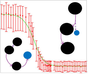
The collision rate of pairs of spheres is given by the integral of the product of the pair-probability density and the inward relative velocity at contact. The pair probability, a measure of the local particle concentration relative to the bulk, and the inward velocity are altered by hydrodynamic interactions. The relative velocity at separations larger than  $2a^*$ determines the trajectory of sphere pairs that must approach from initially large separations and it is driven by the turbulent shear and differential sedimentation. Even without hydrodynamic interactions, Brunk et al. (Reference Brunk, Koch and Lion1998) found trajectories in which pairs on the collision sphere separate and collide again. These closed trajectories should be excluded from the collision rate calculation as only trajectories that begin at large separation are populated by pairs of spheres. Hence, we will perform trajectory analysis, for all cases, to determine the sphere pairs that collide. For numerical efficiency a time reversed flow is considered and sphere pairs start together and move apart, with the trajectory analysis detecting and rejecting those that come back together. We perform a Monte Carlo integration over all possible starting positions in the time-reversed flow and ensemble average over the various realizations of turbulence to obtain the collision rate.
The collision rate is calculated over a large parameter space. We report the ideal collision rate and the collision efficiency, which describes the retardation of collision rate due to hydrodynamic interactions. The former depends on  $Re_{\lambda }$ and the relative strength of differential sedimentation and turbulence. The latter additionally varies with the ratio of the mean-free path
  $\lambda$ to mean sphere radius (the Knudsen number
  $Kn=\lambda /a^*$) and relative size of the interacting spheres. We present results for select parameter values to provide qualitative insight. However, to capture the large amount of data resulting from our simulations we provide a fit for the ideal collision rate and make an analytical approximation to the collision efficiency. This analytical result will be constructed based on an analysis of the pair probability evolution for a special configuration of the sphere pair in the continuum lubrication regime. The collision rate can then be expressed in terms of an integral of the mobilities over radial separation. By cutting off this integral at the approximate separation where continuum breaks down, we will obtain a function that captures important features of the collision efficiency as a function of the various parameters. By adapting this result and fitting the free parameters with the generated collision efficiency data we will obtain a concise and accurate expression for the collision efficiency.
We extend the resulting theory to include the effects of van der Waals interactions in an approximate way by replacing the mean-free path in the original theory with a composite continuum lubrication cutoff separation that incorporates the effects of both non-continuum gas flow and van der Waals forces. The validity of this approximation is tested by comparison with numerical calculations for the pure sedimentation problem from Davis (Reference Davis1984) that incorporates both van der Waals and non-continuum hydrodynamic interactions. This extension makes the theory applicable to particle sizes of the order of 1 to 10  $\mathrm {\mu }$m. The extended theory is then compared with Duru, Koch & Cohen's (Reference Duru, Koch and Cohen2007) experimental measurements of the rate of growth by coalescence of drops falling in an oscillating grid generated turbulent flow. An application of this extended theory is to model the collision process that is critical to filtering pollutants in a spray tower scrubber (see Byeon, Lee & Mohan Reference Byeon, Lee and Mohan2012).
We will obtain the collision rate for spheres settling in turbulent flow. In § 2, we will present the pertinent formulations and outline the procedure to calculate the collision rate. Results for the ideal collision rate with no interparticle interaction will be presented in § 3. We will carry out the calculations with a uniformly valid hydrodynamics, that includes non-continuum lubrication and far-field continuum interactions, in § 4 and present the collision efficiency. The collision efficiency data spanning a large parameter space will be reported with an analytical approximation that will be derived in § 5. Then, in § 6, we will discuss important results from our study and apply the insights to a sample case.
2. Formulation
In a dilute system, the collision of two spheres sets the collision rate  $K_{12}$, given as,
 \begin{equation} K_{12}=-\frac{\textrm{d} n_1}{\textrm{d} t}= C_{12} n_1n_2.\end{equation}
Here,  $n_i$ is the number density of species
  $i$ in the bulk. Shown in (2.1) is the rate of change for ‘1’ assuming collisions with only ‘2’. No ‘1’ species are being formed or lost by other forms of collisions. The two species rate constant
  $C_{12}$ can be expressed by an area integral as,
 \begin{equation} K_{12}= - \int_{(r'=a_1+a_2)\& (\boldsymbol{v}'\boldsymbol{\cdot} \boldsymbol{n}<0)} (\boldsymbol{v}'\boldsymbol{\cdot} \boldsymbol{n}) P'\, \textrm{d} A' .\end{equation}
Here, species  $i$ has radius
  $a_i$ moving with relative velocity of
  $\boldsymbol {v}'$ when separated by a centre to centre distance of
  $r'$. In this paper, we will denote dimensional quantities with a prime and their non-dimensional equivalents without it. At radial separation
  $r'$, the pair probability,
  $P'$, captures the local species concentration relative to the bulk and it takes non-trivial values due to inter-particle interaction. Contributions to the collision rate come only from the radially inward motion when spheres come into contact with each other. This is captured through
  $\boldsymbol {v}'\boldsymbol {\cdot } \boldsymbol {n}<0$, with
  $\boldsymbol {n}$ being the outward normal at the surface on contact.
The equations in our study are scaled with a characteristic length  $a^*=(a_1+a_2)/2$ and a characteristic velocity
  $\varGamma _{\eta } a^*$, where
  $\varGamma _{\eta }=(\epsilon /\nu )^{1/2}$ is the Kolmogorov shear rate,
  $\epsilon$ is the turbulent dissipation rate and
  $\nu$ the kinematic viscosity. Thus, the non-dimensional centre to centre distance
  $r$ ranges from
  $2$ (referred to as the collision sphere) to
  $\infty$ (where one sphere does not influence the other). The strength of gravity is parametrized through
  $Q$, the ratio of characteristic differential-sedimentation velocity to the relative velocity due to turbulent shear. This ratio is defined as
  $Q=(2{\rho _p} g(a_2^2-a_1^2)/[9\mu ])/( \varGamma _{\eta } a^*)$, where
  $g$ is the acceleration due to gravity,
  ${\rho _p}$ is the density of the spheres,
  $\mu$ is the dynamic viscosity experienced by the spheres in the medium. The geometrical parameter, the size ratio given as
  $\kappa =a_2/a_1$, captures the polydispersity of the system and has a range of
  $\kappa \in (0,1]$. Thus the collision rate can be scaled with
  $n_1n_2\varGamma _{\eta } (2a^*)^3$ and expressed through an integral over the collision sphere as,
 \begin{equation} \frac{K_{12}}{ n_1n_2\varGamma_{\eta} (2a^*)^3}= -\int_{(r=2)\& (\boldsymbol{v}\boldsymbol{\cdot} \boldsymbol{n}<0)} (\boldsymbol{v}\boldsymbol{\cdot} \boldsymbol{n}) P \, \textrm{d} A. \end{equation}
It should be noted that this formulation and scaling is valid in the absence of particle and fluid inertia, corresponding to sub-Kolmogorov particles with a low particle response time relative to  $\varGamma _{\eta }^{-1}$. In this inertialess system, the particle relative velocity
  $\boldsymbol {v}$ can be expressed as a linear superposition of terms proportional to the current velocity gradient and gravitational force as,
 \begin{align} v_i &= \varGamma_{ij} r_j - \left[A(r)\frac{r_i r_j}{r^2}+B(r)\left(\delta_{ij}-\frac{r_i r_j}{r^2}\right)\right] \varGamma_{jk} r_k \nonumber\\ &\quad - \left[L(r)\frac{r_i r_j}{r^2}+M(r)\left(\delta_{ij}-\frac{r_i r_j}{r^2}\right)\right] Q\delta_{j3}. \end{align}
The mobility functions  $A(r), L(r), B(r)$ and
  $M(r)$, which are obtained from solutions of the non-continuum gas flow between the particles, describe the relative particle velocity for a specified driving force. Here,
  $A(r),L(r)$ are radial mobilities and
  $B(r),M(r)$ are tangential mobilities for a linear flow and differential sedimentation, respectively. These mobilities take trivial values in the ideal case, i.e. in the absence of particle interactions they are
  $1-A(r)=1-B(r)=L(r)=M(r)=1$. With hydrodynamic interactions these quantities take values between 0 and 1. Gravity is directed along the negative 3-direction. The velocity gradient of the local and instantaneous linear flow experienced by the sub-Kolmogorov spheres in homogeneous isotropic turbulence is denoted as
  $\boldsymbol {\varGamma }$. It has been non-dimensionalized by the Kolmogorov shear rate. It is obtained from the model developed by Girimaji & Pope (Reference Girimaji and Pope1990) that consists of a set of stochastic differential equations to describe the evolution of the fluid velocity gradient in a Lagrangian reference frame. The model describes the evolution over the integral time scale of the pseudo-dissipation rate (sum of squares of the velocity-gradient components) which has a log-normal distribution. The velocity-gradient tensor normalized by the square root of the pseudo-dissipation evolves in a manner that captures the effects of the nonlinear inertial terms in the equations of motion on the relative orientation of the vorticity and straining axes. The model also captures the autocorrelation time of the strain rate observed in DNS of homogeneous, isotropic turbulence. Girimaji & Pope (Reference Girimaji and Pope1990) applied this model to moderate values of
  ${Re}_{\lambda }$ for which the necessary parameters were available from DNS studies. We use the velocity gradient model at higher Taylor microscale Reynolds number by using appropriate values for two of the critical components, the variance of the pseudo-dissipation rate and the ratio of the integral time scale to the Kolmogorov time scale. The variation of these two scalar quantities with
  ${Re}_{\lambda }$ has been studied in DNS (Yeung & Pope Reference Yeung and Pope1989) as well as experiments (Sreenivasan & Kailasnath Reference Sreenivasan and Kailasnath1993). These results have been compiled and a concise expression given in the appendix of Koch & Pope (Reference Koch and Pope2002).
To evaluate the collision rate from (2.3) we also need information on  $P$. This can be obtained from the governing equation,
 \begin{equation} \frac{\partial P}{\partial t}+ \boldsymbol{\nabla} \boldsymbol{\cdot} (\boldsymbol{v} P)= 0,\end{equation}
with the boundary condition  $P \to 1$ as
  $r \to \infty$ corresponding to uncorrelated particles at large separations. Trajectories that start and end on the collision sphere and thus do not extend to
  $r \to \infty$ are set to
  $P =0$. A non-trivial evolution of the pair probability is possible only for a non-solenoidal relative velocity. The solenoidal nature is broken by the hydrodynamic interactions between particles, reflected by non-integer mobilities, leading to
  $P \neq 1$ when
  $r=O(1)$.
The initial state of the sphere pairs constituting equation (2.3) is a large separation from each other. However, it is numerically very expensive to evaluate trajectories of satellite spheres evolving from large separations to  $r=2$ since most of them will miss the test sphere placed at the origin. Hence, exploiting Stokes flow reversibility, a time-reversed calculation is performed. In this time-reversed flow the satellite spheres begin at
  $r=2$ and those that reach the outer boundary, set as
  $r_{\infty }$, without returning to
  $r=2$ will make non-zero contributions towards the integral in (2.3).
In the time-reversed flow the calculations begin by first seeding satellite spheres on the collision sphere. To span the initial angular positions we use a Monte Carlo integration scheme. From randomly chosen initial points on the collision sphere the satellite spheres are evolved using ‘ODE45’, an in-built adaptive time-stepping routine available in MATLAB, which takes as input the relative velocity given in (2.4). This stochastic flow field is updated every  $0.1 /\varGamma _{\eta }$ using the velocity-gradient model. The starting times of the satellite spheres are staggered by
  $1 /\varGamma _{\eta }$ to extensively sample each realization of the turbulent flow field. The satellite spheres only interact with the test sphere and are allowed to evolve for a long time up to
  $150/\varGamma _{\eta }$. By this time more than 99
  $\%$ of the satellite spheres have either reached
  $r=2$ or
  $r=r_{\infty }$, with
  $r_{\infty }$ representing the separation at which sphere pairs no longer influence each other. We find convergent result for the pair probability at contact when
  $r_{\infty }=7$ and so the collision rate can be accurately calculated. The results depend on the specific realization of turbulence in which the satellite spheres evolved. To ensemble average we obtain a different realization of the turbulent flow by changing the starting time by
  $400/\varGamma _{\eta }$. In this way, each of the
  $N_r$ realizations are separated by at least two integral time scales even when
  ${Re}_{\lambda }$ is as high as 2500. The separation is also much larger than the correlation times for both straining and rotational components of the linear flow, which are
  $2.3/\varGamma _{\eta }$ and
  $7.2/\varGamma _{\eta }$, respectively. In addition to the ensemble averaged collision rate we also estimate the error, through the standard deviation
  $\sigma _e$ over the various realizations, and report error bars throughout this paper at the
  $90\,\%$ confidence level.
3. Ideal collision rate
In the absence of hydrodynamic interactions,  $A(r)=0,L(r)=1,B(r)=0,M(r)=1$ and
  $P$ is either 1 or 0. Using this information as input into (2.4), we follow the procedure outlined in § 2 to calculate the collision rate with
  $N_r=200$. For each realization we perform Monte Carlo integration by evaluating 150 trajectories. These satellite spheres, in the time-reversed flow, are assigned
  $P=1$ if they reach
  $r_{\infty }$ within the allotted simulation without going to
  $r=2$ and 0 otherwise.
The ideal collision rate  $K^0_{12}$ is presented as I in figure 1 in the absence of gravity, i.e.
  $Q=0$, as a function of Taylor microscale Reynolds number. It is immediately evident that a non-trivial behaviour is observed, in contrast to the constant collision rate predicted by Saffman & Turner (Reference Saffman and Turner1956). In their analysis a pseudo-steady extensional flow with Gaussian statistics for the strain rate was used. Our result is expected to be more accurate as we use a stochastic flow with statistics of the velocity more closely aligned with the non-Gaussian velocity gradient expected based on the Navier–Stokes equations and observed in DNS.

Figure 1. Case ‘I’ is the ideal collision rate  $K^{0}_{12}$ given as a function of
  ${Re}_{\lambda }$ for
  $Q=0$, i.e. no gravitational effects. The variation of the inward velocity on the collision sphere with Taylor microscale Reynolds number is given by ‘II’. Calculations performed with a frozen velocity gradient during any given satellite sphere evolution are denoted by ‘III’. Case ‘IV’ is the model of Saffman & Turner (Reference Saffman and Turner1956), which is independent of
  ${Re}_{\lambda }$. A portion of the decreased inward velocity can be attributed to changes in
  $\langle \varPhi ^{1/2} \rangle$ as the log normal pseudo-dissipation distribution becomes broader with increasing Taylor microscale Reynolds number. This quantity is continuously decreasing with
  ${Re}_{\lambda }$ and is given as ‘
 $V$’ after multiplying with
  $\int _{(r=2)\& (n_i\varGamma _{ij}n_j<0)} \, \textrm {d} A n_i\varGamma _{ij}n_j/\varPhi ^{1/2} \approx 1.4$. The predictions of the ideal collision rate fit, given in (3.2), are plotted as ‘VI’.
The Taylor microscale Reynolds number,  ${Re}_{\lambda }$, influences the non-Gaussian statistics of the turbulent velocity gradient. This is evident from DNS and experimental studies of the pseudo-dissipation rate
  $\varPhi =\varGamma _{ij}\varGamma _{ij}$ (Yeung & Pope Reference Yeung and Pope1989; Sreenivasan & Kailasnath Reference Sreenivasan and Kailasnath1993). The collision rate is proportional to
  $n_i\varGamma _{ij}n_j\mathcal {H}(-n_i\varGamma _{ij}n_j)$ evaluated on the collision sphere, which is proportional to
  $\langle \varPhi ^{1/2} \rangle$. Here,
  $\mathcal {H}$ is the Heaviside function and the angle brackets indicate an ensemble average. This moment of pseudo-dissipation can be calculated as,
 \begin{equation} \langle \varPhi^{1/2} \rangle = \int P_{\varPhi}\varPhi^{1/2}\, \textrm{d} \varPhi=\frac{\displaystyle\int\epsilon^{{1}/{2}}P_{\epsilon}\, \textrm{d} \epsilon}{\left(\displaystyle\int \epsilon P_{\epsilon}\, \textrm{d} \epsilon\right)^{{1}/{2}}}, \end{equation}
where  $P_{\varPhi }$ is the probability density function for the normalized pseudo-dissipation
  $\varPhi$ and
  $P_{\epsilon }$ is the probability density function for
  $\epsilon$, which is available in the literature (see Koch & Pope Reference Koch and Pope2002). To obtain a result that can be compared with the flux on the collision sphere we multiply (3.1) by the mean normalized flux,
  $\int _{(r=2)\& (n_i\varGamma _{ij}n_j<0)}\, \textrm {d} A n_i\varGamma _{ij}n_j/\varPhi ^{1/2}$, which is approximately 1.4 and independent of
  ${Re}_{\lambda }$. For a detailed derivation of the mean normalized flux please refer to appendix A. This result, which is shown as V in figure 1, decreases with
  ${Re}_{\lambda }$. Increasing
  ${Re}_{\lambda }$ leads to larger tails of the turbulent velocity-gradient probability distribution function and so the expected value for a low-order moment decreases. Since
  $n_i\varGamma _{ij}n_j\mathcal {H}(-n_i\varGamma _{ij}n_j)$ is of lower order than
  $\varPhi$, the observed decrease of the collision rate with
  ${Re}_{\lambda }$ in figure 1 is expected.
Next, we explicitly calculate the actual flux at the collision sphere by substituting  $\boldsymbol {v}'\boldsymbol {\cdot } \boldsymbol {n}=n_i\varGamma _{ij}n_j$ in (2.3). This is the collision rate that would occur in a persistent flow in the absence of closed trajectories. This result, which is the closest analogue to the calculation of Saffman & Turner (Reference Saffman and Turner1956), is shown as II in figure 1. Unlike the result of Saffman & Turner (Reference Saffman and Turner1956), our inward flux varies with
  ${Re}_{\lambda }$ and is lower than the 1.29 prediction of Saffman & Turner (Reference Saffman and Turner1956). While surprising at first glance, it is important to note that most DNS studies validating the Saffman & Turner (Reference Saffman and Turner1956) result are carried out at low
  ${Re}_{\lambda }$ and our calculations show that the deviations in this regime are minimal. Wang, Wexler & Zhou (Reference Wang, Wexler and Zhou1998) performed DNS at
  ${Re}_{\lambda }=24$ and at this point the curve V in figure 1 agrees very well with the published result. Ireland et al. (Reference Ireland, Bragg and Collins2016a) performed DNS over a large range of
  ${Re}_{\lambda }$, from 88 to 597, and found that the inward flux decreased by
  $10\,\%$ with increasing
  ${Re}_{\lambda }$ but this change was within the statistical uncertainty of the DNS. Thus, the results of our stochastic simulations yielding a flux that is decreasing with increasing
  ${Re}_{\lambda }$ is consistent with previous DNS even though the DNS evaluations did not have sufficient statistical accuracy to prove these trends. The flux from the stochastic simulations , II in figure 1, decreases more rapidly with
  ${Re}_{\lambda }$ than the estimate based on the mean value
  $\langle \varPhi ^{1/2} \rangle$,
  $V$ in figure 1. This difference can be attributed to correlations between the normalized velocity gradient and the pseudo-dissipation that can be expected based on the coupled evolution equations in the model (see Girimaji & Pope Reference Girimaji and Pope1990).
The difference between the mean inward flux, II, and the ideal collision rate, I, can be attributed to two factors: the unsteadiness of the flow and the presence, even in a frozen flow, of trajectories that start and end on the collision sphere in the presence of fluid rotation. To distinguish these effects, we compute as III the collision rate in a velocity-gradient field frozen during the satellite evolution. The frozen velocity-gradient result III is much closer to the ideal collision rate I ( $13\,\%$ difference between I and III at large
  ${Re}_{\lambda }$) than it is to the mean inward flow II (
 $33\,\%$ difference between II and III), indicating that closed trajectories are a larger factor in reducing the collision rate than unsteadiness. The decrease in collision rate due to closed trajectories for large
  ${Re}_{\lambda }$ in the Girimaji & Pope (Reference Girimaji and Pope1990) model is approximately
  $42\,\%$ (i.e. difference between I and II), which is much larger than the
  $20\,\%$ change observed in a Gaussian random flow field by Brunk et al. (Reference Brunk, Koch and Lion1998). This suggests that the tendency of the vorticity to align nearly perpendicular to the primary strain rate eigenvector that would be expected in a turbulent flow and the Girimaji & Pope (Reference Girimaji and Pope1990) model increases the prevalence of closed trajectories. Figure 2 shows the ideal collision rate
  $K^0_{12}$ as a function of the strength of gravity
  $Q$. With increasing
  $Q$, the ideal collision rate increases and converges to a line with a slope
  $({\rm \pi} /2)$ and intercept of zero at high
  ${Re}_{\lambda }$. This asymptote corresponds to the ideal pure differential-sedimentation collision rate of
  $2n_1n_2 {\rho _p} g(a_2^2-a_1^2) (a_1+a_2)^2/(9\mu )$ calculated by Smoluchowski (Reference Smoluchowski1918). The convergence to this result with increasing
  $Q$, and the collapse in the dependence of the ideal collision rate on
  ${Re}_{\lambda }$, is expected as gravity is not a stochastic process and it washes away all the intricacies, such as re-circulating trajectories, arising from turbulence. Only
  ${Re}_{\lambda }=90$ and
  $2500$ are shown to avoid crowding in the plot. However, the behaviour described here is valid for a large range of
  ${Re}_{\lambda }$. To concisely capture the large amount of data we have calculated across the parameter space in
  $Q$ and
  ${Re}_{\lambda }$ we use a fitting function. This is given as,
 \begin{equation} \frac{K_{12}^0}{ n_1n_2\varGamma_{\eta} (2a^*)^3}=\frac{f_1{Re}_{\lambda}^{f_2}}{1+f_Q Q}+ \frac{\rm \pi}{2}Q. \end{equation}
Here,  $f_1, f_2$ and
  $f_Q$ are fitting parameters. This form captures the asymptotic behaviour in the large
  $Q$ limit shown in figure 2 and an
  ${Re}_{\lambda }$ power law to fit the
  $Q=0$ limit shown in figure 1. We found that
  $f_1=1.55, f_2=-0.09$ and
  $f_Q=2.1$ give the best agreement with these data. From this expression, it is evident that the coupling of gravity with turbulence leads to a non-trivial result that cannot be captured through a linear combination of the collision rates due to gravity and turbulence acting independently.

Figure 2. The ideal collision rate  $K^0_{12}$ is given as a function of
  $Q$ at
  ${Re}_{\lambda }=90$ and
  $2500$. The symbols correspond to the numerically calculated collision rate and the solid lines to the fit. The higher
  ${Re}_{\lambda }$ corresponds to lower collision rate. For reference, the ideal collision rate predicted by Smoluchowski (Reference Smoluchowski1918) for spheres settling in a quiescent fluid is given by the dashed line.
4. Collision rate with hydrodynamic interactions
Hydrodynamic interactions alter the relative velocity and pair probability and retard the collision rate ( $K^{HI}_{12}$) relative to the ideal flow result. The collision efficiency (
 $\beta =K^{HI}_{12}/K^0_{12}$) will be used to characterize this retardation due to the non-continuum hydrodynamics with the breakdown of continuum parametrized through the Knudsen number,
  $Kn=\lambda _g/a^*$, where
  $\lambda _g$ is the mean-free path of the gas. The mobilities capturing this interaction depend only on the centre to centre distance and, more significantly, the important features are sensitive to the surface to surface distance. For this purpose, a new radial coordinate
  $\xi =r-2$ is used. This coordinate will also be useful to characterize the pair-probability evolution since it is intricately coupled with the mobilities.
Continuum hydrodynamic interaction mobilities have been calculated for the normal direction by Wang et al. (Reference Wang, Zinchenko and Davis1994) by solving for the velocities in a bispherical coordinate system. In the tangential direction
Jeffrey & Onishi (Reference Jeffrey and Onishi1984) and Jeffrey (Reference Jeffrey1992) have presented a twin multipole solution to determine the mobility. Both these series solutions become less accurate as  $\xi$ decreases and so require more terms to compensate. This becomes infeasible in the
  $\xi \ll 1$ limit and, instead, we use the lubrication results available in the literature (see Batchelor & Green Reference Batchelor and Green1972b; Jeffrey & Onishi Reference Jeffrey and Onishi1984; Jeffrey Reference Jeffrey1992). A smooth transition is made between the two regimes.
As the spheres approach each other the continuum lubrication force diverges at a rate that does not allow collision to occur in a finite time (Batchelor & Green Reference Batchelor and Green1972b). The non-continuum lubrication force has a weaker divergence that allows for finite time collisions. Non-continuum effects become important when  $\xi = {O}({Kn})$ and the normal force has been calculated for all separations within the lubrication regime by Sundararajakumar & Koch (Reference Sundararajakumar and Koch1996). We incorporate this non-continuum lubrication result into the normal motion mobilities and obtain a uniformly valid result that captures the breakdown of continuum at
  $\xi \leq {O}({Kn})$, the far-field continuum behaviour when
  $\xi \geq {O}(1)$ and smoothly transitions through continuum lubrication when
  ${Kn}\ll \xi \ll 1$.
In the limit  $\xi \to 0$ continuum tangential mobilities approach a finite value. Hence, in this direction, relative motion is not stalled and the
  ${O}({Kn})$ correction to the mobility is expected to have a small effect on the trajectories. Thus, in our calculation, tangential mobilities are computed based on the continuum hydrodynamics at all
  $\xi$.
The hydrodynamic interactions, both continuum and non-continuum, have an impact on the pair probability. Its evolution along a trajectory can be obtained from (2.5) rewritten as,
 \begin{equation} P=\exp\left(-\int \boldsymbol{\nabla} \boldsymbol{\cdot} \boldsymbol{v}\, \textrm{d} t \right).\end{equation}
Here, the integrand has the divergence of the relative velocity that is given as,
 \begin{align} \frac{\partial v_i}{\partial r_i}&=-\frac{r_i \varGamma_{ij}r_j}{r}\left[3 \frac{A(r)-B(r)}{r}+ \frac{\textrm{d} A(r)}{\textrm{d} r} \right] \nonumber\\ &\quad- Qs_j\delta_{j3}\left[ 2 \frac{L(r)-M(r)}{r}+ \frac{\textrm{d} L(r)}{\textrm{d} r} \right]. \end{align}
 Non-zero contributions to the integral in (4.1) occur when the relative velocity is non-solenoidal. Since  $\boldsymbol {\nabla } \boldsymbol {\cdot } \boldsymbol {v} \to 0$ as
  $r \to \infty$, the pair probability approaches a constant value at large separations. Hence, for numerical purposes, we stop tracking the evolution of
  $P$ beyond a certain radial separation, which we have denoted as
  $r_{\infty }$ at the end of § 2. There, we also discuss the necessity of Monte Carlo integration and ensemble averaging. For the case with hydrodynamic interactions we set
  $N_r=100$ and integrate over 50 trajectory evolutions at each realization of the turbulent flow.
As the spheres approach each other the relative velocity decays to zero, even after including non-continuum gas flow effects, albeit at the very slow rate of  ${O}( 1/\ln [\ln ({Kn}/\xi )])$ which allows for collision in finite time. Due to this decay, numerical issues arise in the time-reversed calculation if the satellite spheres begin very close to the test sphere. Instead, we create an offset collision sphere at
  $r=2+\xi _0$ and seed satellite spheres on it. A sufficiently small offset value
  $\xi _0$ is required to accurately evaluate the collision rate while the value must be large enough to facilitate separation of the pairs in a reasonable time period. We find that
  $\xi _0=10^{-7}$ satisfies both these constraints.
Figure 3 shows that the collision efficiency  $\beta$ decreases monotonically with decreasing
  $Kn$ at
  $\kappa =0.7$ and
  ${Re}_{\lambda }=2500$ for
  $Q=0$ (figure 3a) and
  $Q \to \infty$ (figure 3b). A similar trend is observed for intermediate values of
  $Q$. This behaviour results from the increasing range of radial separations for which the continuum lubrication resistance acts as the mean-free path is reduced relative to the sphere radius. Comparing the two panels it is also evident that collisions driven by differential sedimentation have a lower collision efficiency that depends more strongly on
  $Kn$ than those driven by turbulence alone. These qualitative behaviours have been observed at all values of
  $\kappa$.

Figure 3. The decrease of the collision efficiency  $\beta$ with decreasing
  $Kn$ is shown for
  $\kappa =0.7$ and
  ${Re}_{\lambda }=2500$. Panel (a) is in the pure turbulence limit (
 $Q=0$) and (b) is for the differential-sedimentation limit (
 $Q \to \infty$).
Figure 4 shows the collision efficiency as a function of the size ratio  $\kappa$ at
  $Kn=10^{-3}$ and
  ${Re}_{\lambda }=2500$. As mentioned previously, the result for turbulence dominated flow (
 $Q=0$, figure 4a) has higher efficiency than the gravity dominated regime (
 $Q \to \infty$, figure 4b). In both cases,
  $\beta$ decreases with decreasing size ratio
  $\kappa$ and this behaviour is observed across the entire parameter space of
  $Kn$ and
  $Q$.The probability distribution of the magnitude of the strain rate varies with
  ${Re}_{\lambda }$ and it impacts the collision rate, as noted in the discussion in § 3 on the ideal collision rates. We show its effect on the collision efficiency in figure 5, calculated at
  $Kn=10^{-2}$ and
  $\kappa =0.9$. We plot results for cases in which turbulence dominates (figure 5a), turbulence competes with gravity (figure 5b) and gravity dominates (figure 5c). Only the case in which turbulence and gravity compete shows a statistically significant variation with
  ${Re}_{\lambda }$. Of course, when gravity is strong
  $Q = 10$ we expect that the effects of turbulence and
  ${Re}_{\lambda }$ will be washed away. In the turbulence dominated regime, the linearity of the Stokes flow particle interactions implies that the collision efficiency depends only on the mobility functions and not on the distribution of strain rate magnitudes. At intermediate
  $Q$, changes in the strain rate distribution can alter the relative importance of the linear flow and differential sedimentation mobilities in determining the collision efficiency. At higher
  ${Re}_{\lambda }$, the mean inward velocity due to turbulence is smaller for a given value of
  $\langle \epsilon \rangle ^{1/2}$. This makes the collision efficiency more sensitive to sedimentation mobilities, so that
  $\beta$ decreases with increasing
  ${Re}_{\lambda }$.

Figure 4. The collision efficiency is shown as a function of  $\kappa$ for
  $Kn=10^{-3}$ and
  ${Re}_{\lambda }=2500$. Panel (a) is in the absence of gravitational effects (
 $Q=0$) and (b) is in a purely gravity driven flow (
 $Q \to \infty$).

Figure 5. The dependence of  $\beta$ on
  ${Re}_{\lambda }$ is shown for
  $Kn=10^{-2}, \kappa =0.9$ at (a)
  $Q=0$, (b)
  $Q \approx 1$ and (c)
  $Q \approx 10$. The collision efficiency varies with
  ${Re}_{\lambda }$ for moderate
  $Q$.
$Q$.
Figure 6 shows the variation of  $\beta$ with the strength of gravity
  $Q$ at
  $Kn=10^{-3}, \kappa =0.5$ and
  ${Re}_{\lambda }=2500$. A decrease in collision efficiency with
  $Q$ is observed at all values of
  $Kn, \kappa$ and
  ${Re}_{\lambda }$ we have considered and can be attributed to the difference in the strength of the hydrodynamic interactions.

Figure 6. The variation of the collision efficiency with  $Q$ is shown for
  $Kn=10^{-3}$ and
  $\kappa =0.5$. The symbols correspond to the stochastic linear flow field with
  ${Re}_{\lambda }=2500$. The solid line is the frozen uniaxial compressional flow calculation, with the compression axis aligned with gravity.
Differential-sedimentation hydrodynamic interactions are stronger than those for any linear flow and not just the stochastic linear flow observed by sub-Kolmogorov spheres in turbulence. To demonstrate this  $\beta$ is calculated for a comparable frozen linear flow field. We use a steady compressional flow, the most common realization of the local velocity gradient in turbulent flow (see Ashurst et al. Reference Ashurst, Kerstein, Kerr and Gibson1987). We choose to consider a uniaxial compressional flow whose axis of compression is aligned with the direction of gravity. To determine the compression rate (
 $\dot {\gamma }$) in terms of Kolmogorov quantities we equate the ideal collision rate in static uniaxial compressional flow, calculated by Zeichner & Schowalter (Reference Zeichner and Schowalter1977) and given as
  $[4{\rm \pi} /(3\sqrt {3})]n_1n_2 \dot {\gamma } [2a^*]^3$, with the equivalent turbulent result, evaluated by Saffman & Turner (Reference Saffman and Turner1956) and given as
  $(8{\rm \pi} /15)^{{1}/{2}}(2a^*)^3 n_1n_2(\epsilon /\nu )^{{1}/{2}}$. Thus, we get
  $\dot {\gamma }=(18/[5{\rm \pi} ])^{1/2}(\epsilon /\nu )^{1/2}$. By following a non-dimensionalization consistent with that outlined in § 2 we evaluate
  $\beta$ and
  $Q$ for the static flow field and plot it along with the stochastic result in figure 6. The two calculations generally exhibit similar collision efficiencies across the parameter space in
  $Q$. Around
  $Q \approx 5$, however, the frozen flow field result shows non-monotonic behaviour with
  $Q$. These intricate features in the collision efficiency arise due to satellite spheres moving in circuitous trajectories. They are washed away by the angular variation and time dependence of the strain fields in turbulence. A statistically significant difference in
  $\beta$ between the stochastic and deterministic results is observed for small
  $Q$. This can be attributed to the difference in collision efficiency of the realizations of the linear flow that are not uniaxial compression. This difference is reasonably small suggesting that uniaxial compressional flow does make the dominant contribution.
5. Analytical approximation for the collision efficiency
In § 4, we have presented the collision efficiency  $\beta$ for some typical values of Taylor microscale Reynolds number, size ratio of the spheres, relative strength of gravity to the turbulent flow and strength of non-continuum hydrodynamic interactions. We showed some of the important qualitative features of the variation of the collision efficiency with these parameters but it is not feasible to present data on
  $\beta$ that exhaustively span the parameter space. Hence, in this section, we obtain an analytical approximation to the collision efficiency. The analytically derived expression is based on the pertinent parameters of the collision dynamics:
  $Kn, Q$ and
  $\kappa$. Undetermined constants will be obtained by fitting the available data on
  $\beta$. We have not included
  ${Re}_{\lambda }$ in this analysis as there is no fully theoretical understanding of the velocity-gradient statistics. Instead, we will consider the very high Taylor microscale Reynolds number regime and carry out the analysis at
  ${Re}_{\lambda }=2500$. It is to be noted that the variation of
  $\beta$ with
  ${Re}_{\lambda }$, while statistically significant, occurs over a limited portion of the parameter space and even within this range
  ${Re}_{\lambda }$ is weaker than the variation with the other parameters. Hence, a good approximation of the collision rate at various
  ${Re}_{\lambda }$ may be obtained by multiplying the
  ${Re}_{\lambda }$-dependent ideal collision rate presented in § 3 with the collision efficiency computed for
  ${Re}_{\lambda }=2500$.
Batchelor & Green (Reference Batchelor and Green1972a) obtained an expression for the evolution of the pair probability in an extensional flow and an equivalent analysis for differential sedimentation was performed by Batchelor (Reference Batchelor1982). These analyses involved evaluating an integral that combined the radial and tangential mobilities over radial separation. Continuum lubrication approximations to the mobilities were employed under the assumption that the decrease in the pair probability attenuating the collision rate was dominated by the continuum lubrication regime. Chun & Koch (Reference Chun and Koch2005) used this idea to obtain a closed form expression for the collision efficiency in a linear flow with interactions governed by non-continuum hydrodynamic lubrication. Non-continuum interactions are much weaker than the continuum forces and so it is possible to cut off the collision efficiency integral at  $\xi ={O}(Kn)$. By retaining only the leading-order term in the tangential mobility, they obtained a power law in Kn. To determine the power law pre factor they fitted their expression to the collision efficiency data computed for a monodisperse suspension in a turbulent flow. This result does not account for the difference in size of the interacting spheres or the coupling of turbulence with differential sedimentation. Hence, we derive a more general expression and retain an additional term in the tangential mobility to increase the accuracy of the approximation for
  $\beta$.
The critical components in computing the collision efficiency are the relative velocity and pair probability. The evolution of the latter is given by (2.5), where it is coupled with the former. To evaluate these components and obtain a closed form expression for  $\beta$, we consider trajectories driven by differential sedimentation and a frozen uniaxial compressional flow, the most common linear flow in a turbulent velocity field (see Ashurst et al. Reference Ashurst, Kerstein, Kerr and Gibson1987), whose compressional axis is aligned with gravity. For the sake of convenience, in this frozen flow calculation, we will use spherical coordinates
  $(r,\theta , \phi )$, where
  $\theta$ is the polar angle measured from the direction of gravity and
  $\phi$ is the azimuthal angle measured in the plane normal to gravity. This plane contains both the extensional axes of the uniaxial compressional flow. Without loss of generality, we consider motion only in the
  $\phi =0$ plane and, thus, (2.5) can be written as,
 \begin{equation} v_r\frac{\partial P}{\partial r} +v_{\theta}\frac{1}{r} \frac{\partial P}{\partial \theta}=-P \boldsymbol{\nabla} \boldsymbol{\cdot} \boldsymbol{v}.\end{equation}
Here,  $v_r$ and
  $v_{\theta }$ represent the velocity components in the
  $r$ and
  $\theta$ directions, respectively. Using the method of characteristics and simplifying we get,
 \begin{equation} \ln P = \int^{\infty}_{r^*} -\frac{\boldsymbol{\nabla} \boldsymbol{\cdot} \boldsymbol{v} }{v_r} \, \textrm{d} r,\end{equation}
where  $r^*$ denotes the lower bound of the integral. This integral is to be computed along a trajectory for which
  $(r \sin \theta ) \, \textrm {d}\theta /\textrm {d} r=v_{\theta }/v_r$. Expanding
  $\boldsymbol {\nabla } \boldsymbol {\cdot } \boldsymbol {v}$ and simplifying we get,
 \begin{equation} \int^{\infty}_{r^*} \frac{\boldsymbol{\nabla} \boldsymbol{\cdot} \boldsymbol{v} }{v_r} \, \textrm{d} r= \int^{\infty}_{r^*} d(\ln v_r) + \int^{\infty}_{r^*}\left(\frac{2}{r}+ \frac{1}{v_r}\frac{1}{r \sin \theta} \frac{\partial(v_{\theta} \sin \theta)}{\partial \theta} \right) \, \textrm{d} r.\end{equation}
The relative velocity in spherical coordinates can be given as,
 \begin{equation} \left.\begin{array}{c@{}} v_r = r[1-A(r)](1-3\cos^2\theta) -L(r)Q\cos \theta, \\ v_{\theta} = 3 r[1-B(r)]\cos\theta \sin\theta +M(r)Q\sin \theta. \end{array}\right\}\end{equation}
Incorporating this result into (5.3) and subsequently into (2.3), the collision rate is determined to be,
 \begin{align} \frac{K_{12}}{n_1n_2\varGamma_{\eta} (2a^*)^3}=v_{r,\infty}\exp \left(\int^{\infty}_{r^*} \, \textrm{d} r \left[ \frac{2}{r}+\frac{3[1-B(r)](3\cos^2\theta-1) +2M(r)Q\cos \theta/r}{r[1-A(r)](1-3\cos^2\theta) -L(r)Q\cos \theta} \right] \right).\end{align}
Here,  $v_{r,\infty }$ is the radial velocity at large separations. From this equation, an expression for the ideal collision rate can be obtained and used to determine
  $\beta$. In the
  $\xi ^* \ll 1$ limit, we obtain
 \begin{align} \beta&=\exp\left(\int^{\infty}_{\xi^*} \, \textrm{d} \xi \left[ \frac{3[1-B(\xi)](3\cos^2\theta-1) +M(\xi)Q\cos \theta}{2[1-A(\xi)](1-3\cos^2\theta) -L(\xi)Q\cos \theta} \right.\right. \nonumber\\ &\quad -\left.\left. \frac{3(3\cos^2\theta-1) +Q\cos \theta}{2(1-3\cos^2\theta) -Q\cos \theta} \right] \right). \end{align}
This integral will give  $\beta =0$ when evaluated with
  $\xi ^*=0$ using continuum mobilities. Instead, we use the asymptotic continuum lubrication mobilities in (5.6) and cut the integral off at separations comparable to the mean-free path. From the work of Batchelor & Green (Reference Batchelor and Green1972b) and Batchelor (Reference Batchelor1982), it is known that
  $1-A(\xi ) \approx A_1 \xi , L(\xi ) \approx L_1 \xi$. For tangential mobilities, Jeffrey & Onishi (Reference Jeffrey and Onishi1984) and Jeffrey (Reference Jeffrey1992) showed that
  $1-B(\xi ) \approx B_0+B_1/\ln (\xi ^{-1}), M(\xi )\approx M_0+M_1/\ln (\xi ^{-1})$. While
  $B_0,B_1,M_0,M_1,A_1,L_1$ only depend on
  $\kappa$ we have
  $(r \sin \theta ) \, \textrm {d} \theta / \, \textrm {d} r=v_{\theta }/v_r$ and so only numerical solutions are possible for (5.6). To obtain a closed form expression, we assume
  $\theta$ is not a function of
  $r$, which is applicable to trajectories starting with
  $\theta =0$ or
  ${\rm \pi}$. We hypothesize that the
  $Kn$ dependence of the collision efficiency derived under this approximation will be similar to the exact result for pairs whose orientation evolves with radial separation. Using this approximation and continuum lubrication mobilities we evaluate (5.6). In this way we obtain,
 \begin{equation} \beta=p_1 \frac{{Kn}^{q_1}}{\left(p_2+\ln\dfrac{1}{{Kn}}\right)^{q_2}}.\end{equation}
The exponents are given as,
 \begin{equation} \left.\begin{array}{c@{}} q_1=\dfrac{3 B_0(3\cos^2\theta'-1)+M_0 Q\cos \theta'}{2 A_1(3\cos^2\theta'-1)+L_1 Q\cos \theta'}, \\ q_2=\dfrac{3 B_1(3\cos^2\theta'-1)+M_1 Q\cos \theta'}{2 A_1(3\cos^2\theta'-1)+L_1 Q\cos \theta'}. \end{array}\right\}\end{equation}
The exponent  $q_1$ is associated with the ratio of the leading-order term for the tangential lubrication to the radial lubrication mobility, while
  $q_2$ depends on the next term in the tangential lubrication mobility. These exponents depend on the coefficients of the asymptotic forms of the continuum mobilities, which are given in table 2. The impact of the orientation dynamics of the trajectories evolving under the competition between gravity and turbulence is estimated through
  $\theta '$. This will be used, along with
  $p_1$ and
  $p_2$ which are related to the upper and lower limits of the integral, as free parameters in our calculation.
Table 2. Values of the coefficients in the asymptotic forms of the continuum mobilities:  $B_0,B_1,M_0,M_1,A_,L_1$ at various values of
  $\kappa$. These have been obtained from the work of Jeffrey & Onishi (Reference Jeffrey and Onishi1984), Jeffrey (Reference Jeffrey1992) and Wang et al. (Reference Wang, Zinchenko and Davis1994).

Figures 7(a) and 7(b) show  $\beta$ as a function of
  $Kn$ with
  $\kappa =0.4$ for
  $Q=0$ and
  $Q \to \infty$, respectively. The symbols are the computed results and the line is the analytical approximation, presented in (5.7), with free parameters determined to give best agreement with the data. Note that there is a larger relative change in
  $\beta$ for differential sedimentation than turbulent flow over the range of
  $Kn$. To account for this considerable difference between the two extremes we take
  $p_1, p_2$ to be
  $p_{1,\epsilon }, p_{2,\epsilon }$ and
  $p_{1,g}, p_{2,g}$ for the pure turbulent flow and pure differential-sedimentation cases, respectively. These parameters have been determined by fitting with the computed collision efficiency in the
  $Q=0$ and
  $Q \to \infty$ asymptotes and are presented in table 3 for
  $\kappa$ from 0.3 to 0.99. It should be noted that, in these limits, the analytical approximation is independent of
  $\theta '$. Thus, the fitting parameter
  $\theta '$ will come into play only at finite values of
  $Q$.
$Q$.

Figure 7. The collision efficiency is plotted as a function of  $Kn$ for
  $\kappa =0.4$. Panel (a) is in the pure turbulence limit (
 $Q=0$) and (b) is for pure differential sedimentation (
 $Q \to \infty$). The symbols represent the results of the numerical calculation. The solid lines are the analytical approximation, given in (5.7), which provides a good prediction of the numerical results.
Table 3. Values of the fitting parameters  $p_{1,\epsilon }, p_{2,\epsilon },p_{1,g}$ and
  $p_{2,g}$ at various values of
  $\kappa$.

The dependence of the collision efficiency  $\beta$ on the size ratio
  $\kappa$ is shown in figure 8 for
  $Kn=10^{-2}$, along with the predictions of (5.7). Figure 8(a) shows results at
  $Q=0$ and figure 8(b) is for the
  $Q \to \infty$ limit. To smoothly span size ratios, the parameters
  $p_{1,\epsilon }, p_{2,\epsilon }, p_{1,g}$ and
  $p_{2,g}$ are fitted with a polynomial in
  $\kappa$. The resulting output of (5.7) lies well within the error bounds of the computed numerical data for
  $\kappa \geq 0.3$.

Figure 8. The value of  $\beta$ is shown as a function of
  $\kappa$ at
  $Kn=10^{-2}$. Panel (a) is in the absence of gravitational effects (
 $Q=0$) and (b) is in a purely gravity-driven flow (
 $Q \to \infty$). The symbols represent the results of the numerical calculation with errors bars of
  $\pm \sigma _e/N_r$. The solid line is from (5.7) and agrees well with the data for
  $\kappa \geq 0.3$.
For intermediate  $Q$ values, the fitting parameters,
  $p_1$ and
  $p_2$, in (5.7) are expected to take values between those in the pure turbulent and pure differential-sedimentation regimes. Hence, we take
  $p_1=p_1(Q)$ and
  $p_2=p_2(Q)$, with their functional forms chosen as,
 \begin{equation} \left.\begin{array}{c@{}} p_1(Q)=\exp(-l_1Q)p_{1,\epsilon}+[1-\exp(-l_1 Q)]p_{1,g},\\ p_2(Q)=\exp(-l_2Q)p_{2,\epsilon}+[1-\exp(-l_2 Q)]p_{2,g}. \end{array}\right\}\end{equation}
The best agreement with computed data is found for,
 \begin{equation} \left.\begin{array}{c@{}} \theta'=53^{\circ},\\ l_1=1,\\ l_2=\dfrac{1}{\kappa{Kn}\log\left(\dfrac{1}{{Kn}}\right)}. \end{array}\right\}\end{equation}
 Figure 9 shows the numerical solutions (symbols) for the collision efficiency  $\beta$ as a function of
  $Q$ for
  $\kappa =0.6$ at
  $Kn=10^{-1}$. The line is the result obtained using (5.7) with the form of the free parameters given in (5.9) and values in table 3. The complexity of the fitting function used reflects the underlying complexity of the coupling of the turbulent shear and gravitational settling driving forces in the presence of non-continuum hydrodynamics.

Figure 9. The collision efficiency  $\beta$ is plotted as a function of
  $Q$ for
  $Kn=10^{-1}$ and
  $\kappa =0.6$. The symbols represent the results of the numerical calculation. The solid line is from (5.7), with the fitting parameter forms given in (5.9) and values in table 3. The agreement is good across the parameter space.
In the analysis above, we have considered non-continuum modifications of the viscous resistance as the sole factor allowing coalescence events and so the results are accurate for radii 15  $\mathrm {\mu }$m or larger. Smaller particles are influenced by van der Waals interactions. To incorporate this colloidal attraction, we determine the gap between the drops
  $h^*_{vdW}$ at which the relative radial velocity is doubled relative to the prediction for pure continuum–hydrodynamic interactions. The modified (5.4) that includes the radial mobility for colloidal interactions
  $G(r)$, and the central potential
  $\varPhi _{12,vdW}$ is given as,
 \begin{equation} {v_r = -(1-A(r))r (3\cos^2\theta-1)-\frac{G(r)}{N_F}\frac{\textrm{d}\varPhi_{12,vdW}}{\textrm{d} r} -QL(r)\cos\theta}.\end{equation}
Here,  $N_F=3{\rm \pi} \dot {\gamma } a_1^3\kappa (1+\kappa )\mu /(2\hat {A})$ is the relative strength of viscous shear to van der Waals forces,
  $\hat {A}$ is the Hamaker constant and
  $\dot {\gamma }=(18/[5{\rm \pi} ])^{1/2}(\epsilon /\nu )^{1/2}$ derived in § 4 is used. In the lubrication regime (5.11) becomes,
 \begin{equation} {v_r\sim- 2A_1\xi(3\cos^2\theta-1)-\frac{\xi}{N_F}\frac{(1+\kappa)^2}{2 \kappa}\frac{\kappa}{3(1+\kappa)^2}\frac{1}{\xi^2} -QL_1\xi\cos\theta}.\end{equation}
From (5.12)  $h^*_{vdW}$ is determined as the value of
  $\xi$ at which the van der Waals contribution balances the maximum of the sum of the other two terms, preventing particle separation. The van der Waals velocity component is always inward in this regime but the continuum lubrication velocity can take either sign, depending on the values of
  $Q_2$ and
  $\theta$. The maximum positive value of the continuum velocity occurs when
  $\cos \theta$ is
  $-Q_2/6$ for
  $Q_2<6$ and 1 for
  $Q_2>6$. Here,
  $Q_2=QL_1/2A_1$. From this we get,
 \begin{align} \frac{h^*_{vdW}}{\sqrt{\hat{A}/(18 {\rm \pi}\mu a^3 \kappa(1+\kappa) \dot{\gamma})}} &=\sqrt{\frac{12}{Q_2^2+12}} \quad Q_2<6 \nonumber\\ & =\frac{1}{\sqrt{Q_2-2}} \quad Q_2>6 . \end{align}
In the  $Q=0$ limit (5.13) reduces to
  $h^*_{vdW,\epsilon }$ given as
  $a^* \sqrt {\hat {A}/(18 {\rm \pi}\mu a^3 \kappa (1+\kappa ) \dot {\gamma })}$. In the pure differential regime it is
  $h^*_{vdW,g}$ expressed as
  ${[(1+\kappa )/(2a^*)] \sqrt {\hat {A}/(4{\rm \pi} L_1} {\rho _p} {\kappa (1-\kappa ^2)g)}}$. Equation (5.13) can be used to find a composite Knudsen number
  $Kn_{comp}=(\lambda _g+h^*_{vdW})/a^*$ which, in turn, can be used to obtain the collision efficiency using the procedure outlined earlier in this section.
The analytical model developed here is tested against data available in literature. The computational result for the efficiency of differential-sedimentation-driven collisions from Davis (Reference Davis1984) can be compared with our results in the  $Q \to \infty$ limit. An experimental study by Duru et al. (Reference Duru, Koch and Cohen2007) on coalescence-driven droplet growth in grid generated turbulence has coupled turbulence and differential-sedimentation-driven collisions that test our results for
  $Q=O(1)$. Van der Waals forces and non-continuum interaction play important roles in both comparisons.
Davis (Reference Davis1984) computed the collision efficiency for a sedimenting droplet pair with finite particle inertia interacting via non-continuum hydrodynamic interactions modelled using a Maxwell slip approximation and van der Waals forces. We repeated these calculations for the case where  $a_1=10~\mathrm {\mu } \textrm {m}$ but neglecting particle inertia. The comparison of these results in figure 10 indicates that particle inertia, for all size ratios considered, plays a negligible role when the larger drop is of the chosen size. Next, we apply the analytical model using the composite effective Knudsen number,
  $Kn_{comp}$, with the van der Waals length scale obtained from (5.13). In the
  $Q \to \infty$ limit this length scale reduces to
  $h^*_{vdW,g}$.The model agrees very well with the full calculation, confirming the accuracy of the method used to approximate the coupled effects of van der Waals and non-continuum hydrodynamic interactions. That the coalescence events in the present case have substantial contributions from both mechanisms is also evident from the model. Applying the model for a non-continuum gas in the absence of van der Waals attractions, i.e. replacing
  $Kn_{comp}$ with
  $Kn$, and considering van der Waals attractions in a continuum gas, i.e. replacing
  $Kn_{comp}$ with
  $h^*_{vdW,g}/a^*$, yields comparable values of the collision efficiency.

Figure 10. The collision efficiency  $\beta$ for differential-sedimentation-driven collisions with
  $a_1=10~\mathrm {\mu } \textrm {m}$. The analytical model results for van der Waals attractions and non-continuum hydrodynamic interactions (model:
  $vdW+NC$), non-continuum hydrodynamic interactions without van der Waals forces (model:
  $NC$) and van der Waals attractions in a continuum gas (model:
  $vdW$) are plotted as a function of the size ratio and compared to results of Reference DavisDavis's (Reference Davis1984) trajectory analysis with
  $vdW+NC$ and particle inertia. The composite model (model:
  $vdW+NC$) is in good agreement with the computational result. Our own trajectory analysis with
  $vdW+NC$ and without particle inertia is very close to the results of Davis (Reference Davis1984), indicating that particle inertia is negligible for this drop size.
Duru et al. (Reference Duru, Koch and Cohen2007) measured the size distribution of oil droplets with mean radii in the range 1–2.5  $\mathrm {\mu }$m settling in an oscillating grid generated turbulent flow of a nitrogen gas at various turbulence intensities. The initial polydispersity of the drops was approximately 10 % and the effects of differential sedimentation and turbulent shear judged from the ideal collision rates were comparable. For an initial mean size of
  $a_0$ they find the short time linear growth of the mean droplet radius
  $\langle a\rangle$ and report
  $b=(1/a_0)\, \textrm {d} \langle a\rangle / \textrm {d} t$. This result divided by the number density can be related to integrals of the rate constant over the drop size distribution. Thus, a theoretical prediction of
  $b/n_i$ can be obtained from (17) of Duru et al. (Reference Duru, Koch and Cohen2007) that takes
  $K_{12}$ as an input. We make theoretical predictions of
  $b/n_i$ using our collision rate constant and compare them against experimental data in figure 11. We excluded from this comparison a few of the experimental results for the smallest
  $a_0$ values which were influenced by Brownian motion.

Figure 11. Experimentally evaluated  $b/n_i$ from Duru et al. (Reference Duru, Koch and Cohen2007) is plotted against the initial mean particle size reported in experiments and compared against the theoretical predictions obtained using our
  $K_{12}$. In (a) we show results for a Kolmogorov shear rate of 88 s
 $^{-1}$. The ‘
 $\times$’ are the experimental results, the filled circles are
  $b/n_i$ computed using the ideal result and the open circles are
  $b/n_i$ evaluated with
  $K_{12}^{NC+vdW}$. In (b) we show results for the Kolmogorov shear rate of 88 s
 $^{-1}$ in green, 59 s
 $^{-1}$ in red and 25 s
 $^{-1}$ in blue. The ideal result is not shown here for the sake of conciseness.
Figure 11(a) shows a comparison of the model with experimental measurements of the droplet growth rate for the largest Kolmogorov shear rate of 88 s $^{-1}$ and a range of initial mean drop sizes
  $a_0$. The measured droplet growth (
 $\times$ symbols) increases with
  $a_0$ as a result of the increasing influence of differential sedimentation. The variability of the rate of increase may be attributed in part to variations in the breadth of the drop size distribution. The initial standard deviation of the drop size distribution was also measured and is used in the model calculations. The model calculation yields the open circles which are very similar in magnitude to the experimental measurements and grow at a comparable rate with increasing
  $a_0$. It is notable that the droplet growth rate using the ideal collision rate (filled circles) is much larger than both the experimental measurements and the full model predictions highlighting the importance of interparticle interactions in modulating the coalescence rate. To probe the influence of the turbulence intensity, figure 11(b) provides a comparison of experimental measurements for Kolmogorov shear rates of 25, 59 and 88 s
 $^{-1}$ with the full model predictions. The theory and experiments show an increase in droplet growth rate with increasing turbulent shear rate. The dependence on shear rate is less obvious and systematic at the larger sizes where the sedimentation driving force for collisions may play a larger role. Thus, the theoretical model provides a good representation of experimentally measured droplet coalescence rates in a regime with mixed sedimentation and turbulent shear-driven collisions and mixed van der Waals and non-continuum viscous resistance mechanisms allowing droplet contact.
6. Discussion and summary
We have studied the collision rate of inertialess drops or particles due to the coupled effects of differential sedimentation and turbulent shear flow. The hydrodynamic interactions of the drops include non-continuum lubrication forces allowing particle contact in the absence of non-hydrodynamic attractive forces. In the absence of gravity, we discovered that the ideal collision efficiency decreases with increasing  ${Re}_{\lambda }$, as discussed in § 3, as a result of the non-Gaussian nature of the turbulent velocity-gradient field. The inclusion of gravity led to an ideal collision rate that differs significantly from a linear superposition of the collision rate due to turbulent shear and differential sedimentation acting independently. The consideration of non-continuum hydrodynamic interactions in § 4 leads to a collision efficiency that depends strongly on the Knudsen number
  $Kn$, the relative strengths of gravity and turbulence
  $Q$ and the particle size ratio
  $\kappa$. To concisely report data across the large parameter space we develop, in § 5, an analytical approximation for the collision efficiency.
While the well-known prediction of the ideal collision rate in turbulence at  $Q=0$ based on a Gaussian approximation to the velocity gradient by Saffman & Turner (Reference Saffman and Turner1956) is independent of
  ${Re}_{\lambda }$, our simulations using the Lagrangian velocity-gradient model developed by Girimaji & Pope (Reference Girimaji and Pope1990) indicate that the ideal collision rate decreases by nearly
  $28\,\%$ as the Reynolds number is increased from 90 to 2500. Increasing Taylor microscale Reynolds number leads to larger tails in the probability distribution of turbulent velocity gradients for a given dissipation rate. The dissipation rate is a measure of the mean-square strain rate, while the collision rate depends on the mean inward straining motion at a given location and is thus a lower-order moment. The broader distribution naturally gives rise to a smaller value of this low-order moment and a lower collision rate. While it would be interesting to see how the ideal collision rate depends on the choice of Lagrangian velocity gradient model, we believe that the recent developments in such models (Pereira, Moriconi & Chevillard Reference Pereira, Moriconi and Chevillard2018) that improve the predictions of high-order moments may not have a great influence on the low-order moment that controls the collision rate.
The inclusion of gravity increases the non-dimensional collision rate. However, with increasing  $Q$, the stochastic fluctuations in the relative velocity driven by the turbulent velocity field become less important and the collision rate dependence on
  ${Re}_{\lambda }$ vanishes in the differential-sedimentation dominated regime.
Hydrodynamic interactions significantly retard the collision rate and introduce strong dependence on  $Kn$ and
  $\kappa$. The collision efficiency
  $\beta$, unlike the ideal collision rate, decreases with increasing
  $Q$. At moderate
  $Q$ the complex coupling between the two driving mechanisms and hydrodynamic interactions leads to a statistically significant dependence of
  $\beta$ on
  ${Re}_{\lambda }$. This illustrates the nonlinear change of the collision rate with
  $Q$ and the non-trivial interplay between sedimentation- and turbulence-driven particle motions in the presence of non-continuum hydrodynamic interactions.
Since the collision efficiency depends on multiple parameters, each of which are extensively spanned, it is not possible to report results across the full parameter space concisely. Instead, we develop an analytical approximation to  $\beta$. This has been derived based on an approximate treatment of the evolution of the pair probability along trajectories in the continuum lubrication regime. The separations at which continuum lubrication is considered to begin and end, the angle of the colliding particles and two parameters governing the transition from turbulent shear to gravity dominated collisions provide free parameters used to fit the approximate solution to a wide range of numerical results.
The analytical result for the collision efficiency also provides an intuitive understanding of its dependence on the Knudsen number and the size ratio. The power law dependence of the collision efficiency on the Knudsen number is associated with the power law variation of the pair probability with radial position in the lubrication regime resulting from the functional form of the mobilities. The power law decrease in  $\beta$ with decreasing
  $Kn$ predicted in (5.7) is seen in figures 3 and 7.
With decreasing  $\kappa$ we find, from table 2, that the ratios of the tangent to normal mobilities,
  $M_0/L_1$ for differential-sedimentation-driven collisions and
  $B_0/A_1$ for turbulent collisions, decrease. This suggests that smaller spheres will have less ability to move tangent to one another to an angular position at which they may separate before the normal motion brings them together. As a result, smaller size ratio pairs have a lower collision efficiency. The ratio of the differential-sedimentation mobilities is more sensitive to
  $\kappa$ than that of the turbulent shear mobilities and as a result the decrease in
  $\beta$ with decreasing
  $\kappa$ is stronger for differential sedimentation.
The dependence of the collision efficiency on size ratio can be understood by considering the relative motion of a pair in which one particle is substantially smaller than the other. In this case, the resistance to the centre of mass motion of the pair is dominated by the resistance of the larger particle and the centre of mass velocity becomes close to the terminal velocity of the large particle. The small particle's motion relative to the larger particle is then driven by the fluid flow around the large particle. The tangential fluid velocity around the large sphere is a simple shear flow at small separations. Thus, the fluid velocity that drives the tangent motion of a small sphere is proportional to  $\kappa$ when the small particle is in a lubrication interaction with the large one. The tangent mobility is finite as
  $\xi \to 0$ and the sphere rolls at an
  $O(\kappa )$ speed. The normal fluid velocity pushing the small sphere toward the surface is a quadratic function of the separation of the centre of the small sphere from the large particle surface so the small particle experiences a normal force
  $F' = \kappa ^2$. The normal velocity of the lubricating particle due to this force is
  $F'\xi /\kappa ^2$ (or in dimensional form
  $F'h'/(\mu a_2^2)$, where
  $h'$ is the dimensional surface to surface radial separation and
  $a_2<a_1$). Thus the normal velocity is
  $\xi$, independent of
  $\kappa$ for small
  $\kappa$ and
  $A_1$ or
  $L_1$ is
  $O(1)$. We see then that a small particle rolls around the large particle at a slower
  ${O}(\kappa )$ speed but retains an
  $O(\xi )$ normal velocity. Hence, the exponent in (5.7) and thus the collision efficiency become smaller at smaller
  $\kappa$. The ability of tangential motion to facilitate motion away from the region of inward velocity before normal motion leads to contact is attenuated as the small particle's radius decreases.
If the size ratio becomes small enough, there is a range of separations where  $h'\ll a_1$, for
  $a_2<a_1$, so that the hydrodynamic interactions are strong and alter the pair distribution function significantly but
  $h'\leq {O}(a_2)$ so that the particles are not yet in a lubrication interaction. As a result, there would be a significant change of
  $P$ that is not captured by applying (5.7), which is based on lubrication scalings and would explain the rapid change in
  $p_1$ shown in table 3. Thus, the discussion in the previous paragraph should be taken as a physical interpretation for moderately small
  $\kappa$ rather than a guide to
  $\beta$ for
  $\kappa \ll 1$.
To understand why the collision efficiency for differential sedimentation is smaller and has a stronger  $Kn$ dependence than that for turbulent shear flow, we analyse the fluid flow around a large particle that drives the motion of a smaller particle. For turbulent flow, we consider the most common local flow, a uniaxial compressional flow (see Ashurst et al. Reference Ashurst, Kerstein, Kerr and Gibson1987). The compressional flow has stagnation points at 0, 90 and 180 degree angles relative to the compressional axis, while the flow past a sedimenting particle has stagnation points at 0 and 180 degrees relative to the direction of gravity. Based on mass conservation, we expect the radial velocity of the fluid near the large particle that drives the small particle's normal motion will be larger relative to the tangential velocity when the angular velocity varies more rapidly with angular position. Thus, the particle pair in turbulent shear flow experiences a stronger normal motion driving collision than the pair experiencing differential sedimentation. A weaker normal motion for differential sedimentation leads to a small collision efficiency and the form of the power law exponent in (5.7) indicates that
  $\beta$ will also have a stronger
  $Kn$ dependence in this case.
The fit of the analytical result has been carried out using data on  $\beta$ at
  ${Re}_{\lambda }=2500$ over
  $Kn$ from
  $0.2$ to
  $10^{-4}, \kappa$ from 0.3 to 0.99 and
  $Q$ ranging from 0 to
  $10^5$. Hence, the analytical result is expected to be very accurate and the collision efficiency at intermediate values of the parameters can be obtained through interpolation. This is supported by the trends of
  $\beta$ across
  $\kappa ,Q$ and
  $Kn$ being smooth. This is true of the
  $\beta$ data not shown here and so the analytical approximation is expected to perform well when spanning the parameter space. Additionally the smooth behaviour of the continuum near-field mobility coefficients and the fitting parameters, with respect to
  $\kappa$, gives further credence to the idea that the same qualitative behaviour will be observed across the parameter space and an interpolation of the fitting function will be able to capture
  $\beta$ accurately.
Non-continuum hydrodynamics accurately described droplet interaction for droplet radii of 15  $\mathrm {\mu }$m or larger. To extend our model to smaller sizes we have incorporated van der Waals interactions. While a full analysis of droplet trajectories incorporating both van der Waals and non-continuum hydrodynamic interactions is beyond the scope of this study, we proposed an approximate theory near the end of § 5. This theory is based on a compound effective Knudsen number that depends on the characteristic interdroplet gap at which van der Waals interactions modify the trajectories as well as the mean-free path. The validity of this approximation is confirmed by comparing with full trajectory calculations of the collision efficiency for differential sedimentation performed by Davis (Reference Davis1984). To test the theory for mixed turbulence- and sedimentation-driven collisions in the presence of both non-continuum hydrodynamic and van der Waals interactions, we predict the rate of growth of droplets settling in grid generated turbulence observed by Duru et al. (Reference Duru, Koch and Cohen2007). The magnitude of the predicted growth rate and its dependence on turbulent shear rate and droplet mean radius are in good agreement with the experimental measurements confirming the applicability of our results.
The results of our study can be used to model the collision-coalescence growth of droplets in clouds. Of particular interest is the ‘size gap’ from 15 to 40  $\mathrm {\mu }$m radius, where droplets are large enough that condensational growth is ineffective but still too small to experience rapid gravitational collision. One of the unanswered questions about the ‘size gap’ relates to the time taken for rain formation in warm clouds. Experimental studies suggest that drops grow faster than expected from purely gravity-driven collision (see Langmuir Reference Langmuir1948; Kolmogorov Reference Kolmogorov1962; Beard & Ochs III Reference Beard and Ochs III1993; Blyth et al. Reference Blyth, Lasher-Trapp, Cooper, Knight and Latham2003; Siebert et al. Reference Siebert, Wendisch, Conrath, Teichmann and Heintzenberg2003). Aerosol nuclei grow into drops with sizes up to approximately 15
  $\mathrm {\mu }$m radius by condensation. Condensation leads to faster growth of smaller drops and so it leads to a nearly monodisperse drop size distribution, enhancing the importance of turbulent shear relative to gravity-driven coalescence. For example, a droplet pair with
  $a_1=20~\mathrm {\mu } \textrm {m}$ and
  $\kappa =0.99$ in a turbulent environment with an instantaneous
  $\epsilon$ value of
  $0.1\ \textrm {m}^2\ \textrm {s}^{-3}$ will have a ratio of gravity- to shear-driven coalescence of
  $Q \approx 0.6$. Thus models that rely on differential-sedimentation-driven collision and do not properly account for coupling with turbulence will predict unrealistically large characteristic times for collision events and crossing the ‘size gap’. While simple inclusion of the coupled effects of turbulence and gravity in an ideal collision rate would help to resolve this unrealistically large coalescence growth time prediction, hydrodynamic interactions also play a crucial role in making a more physically accurate estimate. The time to cross the ‘size gap’ is expected to be lower still as particle inertia, through preferential concentration and alteration of the collision dynamics, leads to higher rates (Davis Reference Davis1984; Ireland et al. Reference Ireland, Bragg and Collins2016a).
For the droplets of interest in clouds the breakdown of continuum upon close approach plays a critical role (Sundararajakumar & Koch Reference Sundararajakumar and Koch1996) and has not received extensive treatment in the previous literature. These issues can be resolved through the use of the collision rate presented in this study that properly accounts for non-continuum lubrication, far-field hydrodynamic interactions and the coupled effects of gravity and turbulent flow. Since our study spans a large parameter space in  $Q, Kn$ and
  $\kappa$ it will be adept at resolving some of the important features of the evolution of the droplet spectra in the ‘size-gap’ regime where both gravity and turbulence are expected to be important and many values of the mean radius and radius ratio need to be considered.
Our collision rate results indicate a significant growth rate of droplets through the ‘size gap’. The collision efficiency is larger for turbulence dominated than gravity dominated collisions and larger for nearly equal size spheres than for those with a small size ratio. Both these factors tend to decrease the variability of the overall collision rate and facilitate collisions between nearly equal size 15  $\mathrm {\mu }$m radius drops that must coalesce for the drops to grow and the size distribution to become more polydisperse following the condensation growth.
Our study, in addition to rates and efficiency, provides a route to subgrid modelling in clouds. The large scale dynamics can be simulated with DNS, a large eddy simulation or other established techniques. The finer details of collision on the particle scale, many orders of magnitude smaller than the integral scales of turbulence, can be solved using the collision rates obtained here. Since the present study neglects particle inertia, it is most applicable to drops in the lower portion of the ‘size gap’ (15 to 25  $\mathrm {\mu }$m radii) in moderately turbulent clouds, as indicated in table 1, where condensation leads to a relatively monodisperse distribution. A study of larger drops with greater polydispersity whose collisions are driven by differential sedimentation and influenced by particle inertia (Davis Reference Davis1984) would complement the present model. The two results together might then span the full ‘size-gap’ range. It would also be of interest to contrast the present analysis of droplet coalescence in a Lagrangian reference frame with a future study of the collision rate of rapidly settling droplets in a low turbulence cloud to highlight the effect of the Froude number on the coalescence rate.
Acknowledgements
The authors thank U. Menon for sharing the algorithm to implement the velocity-gradient model.
Funding
This work was supported by NSF grants 1435953 and 1803156.
Declaration of interest
The authors report no conflict of interest.
Appendix A. Mean normalized flux of particle pairs at the collision surface
The mean flux of particle pairs on the collision surface,  $\int _{ n_i v_i<0}\, \textrm {d} A |n_i v_i|$, consists of the root-mean-square pseudo-dissipation,
  $\varPhi ^{1/2}$, which depends on
  $Re_{\lambda }$ and a prefactor,
  $m$, which is independent of
  $Re_{\lambda }$ for the ideal collision rate at
  $Q=0$. In this section1 we will calculate this prefactor. Dividing the mean flux by
  $\varPhi ^{1/2}$ gives the mean normalized flux
  $m=\langle C_{ij}h_{ij} \rangle$. Here,
  $\boldsymbol {h}=\boldsymbol {\varGamma }/\varPhi ^{1/2}$ is the normalized velocity gradient and
  $C_{ij}$ is defined as,
 \begin{equation} {C_{ij}=\int_{ n_ih_{ij}n_j<0}\, \textrm{d} A n_i n_j}.\end{equation}
 The normalized velocity gradient,  $\boldsymbol {h}$, is a sum of straining
  $\boldsymbol {s}$ and rotational
  $\boldsymbol {r}$ components, i.e.
  $\boldsymbol {h}=\boldsymbol {s}+ \boldsymbol {r}$. In conjunction with incompressibility, the constraints on
  $\boldsymbol {h}$ at the collision sphere are,
 \begin{align} &{\langle h_{ij} \rangle=0}, \end{align}
 \begin{align} &{ \langle h_{ij} h_{ij} \rangle=1}. \end{align}
Similarly, the constraints on the straining component for isotropic turbulence are,
 \begin{align} &{\langle s_{ij} \rangle =0}, \end{align}
 \begin{align} &{\langle s_{ij} s_{ij} \rangle =0.5}. \end{align}
A tensorial expression for  $C_{ij}$ based on the symmetry of the sphere can be given as,
 \begin{equation} {C_{ij}=\lambda_1 s_{ij}+\lambda_2 r_{ij}+\lambda_3 \delta_{ij}}.\end{equation}
We have  $\lambda _2=0$ since rotation is anti-symmetric while
  $\boldsymbol {C}$ is symmetric. To evaluate
  $\lambda _1$ we multiply
  $C_{ij}$ by
  $s_{ij}$ and from
  $\langle s_{ij}s_{ij} \rangle = \langle r_{ij}r_{ij} \rangle =0.5 \langle h_{ij} h_{ij} \rangle$ we get
  $\lambda _1=2\int _{ n_i s_{ij} n_j<0}\, \textrm {d} A n_i s_{ij} n_j$.
Approximating the local strain as uniaxial compression and using the constraints in (A5), an expression for  $\boldsymbol {s}$ can be obtained. This is given as,
 \begin{equation} {\boldsymbol{s} = \frac{\sqrt{3}}{2}\begin{bmatrix} \frac{-1}{3} & 0 & 0\\ 0 & \frac{-1}{3} & 0\\ 0 & 0 & \frac{2}{3} \end{bmatrix}}.\end{equation}
Using this we get  $\lambda _1=8{\rm \pi} /9$. Similarly, we obtain
  $\lambda _3=4{\rm \pi} /3\sqrt {3}$. Thus
  $\boldsymbol {C}=8{\rm \pi} \boldsymbol {s}/9+4{\rm \pi} /3\sqrt {3}\boldsymbol {\delta }$ and so
  $m=4{\rm \pi} /9 \approx 1.4$.


