Introduction
Long-term prediction models developed in the past on the basis of monthly median measurements recorded at various ionospheric observatories are able to provide such reliable climatological predictions of the main ionospheric parameters that they do not require further improvements today. Some of them are regional (Hanbaba Reference Hanbaba1999 and references therein) others, such as the International Reference Ionosphere (IRI; Bilitza & Reinisch Reference Bilitza and Reinisch2008, Bilitza Reference Bilitza2015) and the NeQuick2 (Nava et al. Reference Nava, Coisson and Radicella2008 and references therein), are global.
The importance of short-term forecasting models (Stanislawska & Zbyszynski Reference Stanislawska and Zbyszynski2002, Pietrella & Perrone Reference Pietrella and Perrone2008, Pietrella Reference Pietrella2012, Reference Pietrella2014), providing predictions for a few hours ahead, as well as nowcasting models (Araujo-Pradere et al. Reference Araujo-Pradere, Fuller-Rowell and Codrescu2002, Zolesi et al. Reference Zolesi, Belehaki, Tsagouri and Cander2004, Pietrella & Perrone Reference Pietrella and Perrone2005) that provide real-time predictions, has also been acknowledged by the scientific community, especially in cases of a very disturbed ionosphere when the long-term models are unable to provide reliable forecasts.
The challenge today is the achievement of a comprehensive real-time 3-D specification of the ionosphere (nowcasting). In recent years, the increasing number of digisondes equipped with software that provides automatic real-time scaling of the main ionospheric parameters (Reinisch & Huang Reference Reinisch and Huang1983, Pezzopane & Scotto Reference Pezzopane and Scotto2007) has made it possible to develop nowcasting models the need of which is well recognized. To this regard a large number of models that ingest real-time data and then provide an updated 3-D mapping of the ionosphere has recently proposed (Galkin et al. Reference Galkin, Reinisch, Huang and Bilitza2012, Pezzopane et al. Reference Pezzopane, Pietrella, Pignatelli, Zolesi and Cander2013).
The dataset considered in this study comprises a limited sample of ionograms which were provided within the framework of the Automatic Scaling of Polar Ionograms and Co-operative Ionospheric Observations (AUSPICIO) project and recorded principally in 2001 and 2009, and to a lesser extent in 2006–07 and 2012–15. Different epochs relative to these years, characterized by quiet and disturbed geomagnetic conditions, were selected and analysed during the winter and summer.
The ionograms under consideration were recorded by different types of ionosondes including the Digital Portable Sounder DPS-4 (Haines & Reinisch Reference Haines and Reinisch1995), the IPS 42 (Titheridge Reference Titheridge1993), the AIS-INGV (Zuccheretti et al. Reference Zuccheretti, Tutone, Sciacca, Bianchi and Arokiasamy2003) and the Canadian Advanced Digital Ionosonde (CADI; McDougall Reference McDougall1997). Table I summarizes the ionospheric observatories, the types of ionosonde and the scientific communities involved in providing data.
Table I List of stations involved and their geographical co-ordinates.

a Located inside the Antarctic Polar Circle.
The aim of this work is to assess the performance of the IRI2012 and NeQuick2 models, mainly at high latitudes and inside the Antarctic Polar Circle (APC). However, considering that the Australian Ionospheric Prediction Service also made data available from the mid-latitude stations of Hobart and Macquarie Island, the opportunity was taken to also investigate the behaviour of the models at these stations. Therefore, the ionograms considered in this study were recorded at the ionospheric observatories of Hobart and Macquarie Island (mid-latitude), Comandante Ferraz and Livingstone Island (high latitude), and Casey, Mawson, Davis and Scott Base (APC).
The Autoscala software, dedicated to the automatic scaling of ionograms (Scotto & Pezzopane Reference Scotto and Pezzopane2002, Scotto Reference Scotto2009), was run on the ionograms recorded at the above-mentioned ionospheric observatories. Specifically, the Adaptive Ionospheric Profiler (AIP), which is an integral part of Autoscala, was applied to extract from each ionogram a real-time autoscaled electron density profile, Ne(h), which, in this study, is assumed to be the measured Ne(h); hereafter also referred to as the reference Ne(h) or simply the AIP profile.
Before starting evaluation of the performance of IRI2012 and NeQuick2, a preliminary check was carried out for each observatory to exclude any profiles provided by the AIP routine that were considered unreliable, and those retained were then selected and used as reference profiles.
This was necessary due to the complexity of the structure and dynamics of the high latitude ionosphere, which often gives rise to ionograms that are more diverse and difficult to interpret and autoscale than those recorded at mid-latitudes. This subject is discussed in more detail later in this paper. In these cases, the AIP does not succeed in providing a reliable Ne(h). Some examples of ionograms from which the AIP is not able to provide a reference Ne(h) are presented in Fig. 1.
The selected AIP profiles (some examples of which are also shown in Fig. 2) were compared with: i) the Ne(h) output by the climatological models NeQuick2 and IRI2012, taking as input the F10.7 solar activity index and ii) the Ne(h) provided by the NeQuick2 and IRI2012 models when used as assimilative models, ingesting the values of the critical frequency of the F2 layer (foF2) and the maximum height of the F2 layer (hmF2) obtained automatically in the ionogram inversion procedure used by Autoscala, which is fully discussed by Scotto (Reference Scotto2009).
To include cases characterized by disturbed magnetic/ionospheric conditions, IRI2012 was employed with the STORM option set to ‘ON’. Some example comparisons between the AIP profiles and the NeQuick2 and IRI2012 Ne(h) in both long-term and real-time prediction mode are also shown. The comparisons between NeQuick2 and IRI2012 performance, evaluated in terms of root mean square error (r.m.s.e.), are shown for each ionospheric observatory.
Data ingestion technique
The technique allowing the ingestion of the F2 ionosphere layer parameters, i.e. foF2 and hmF2 deduced from ionosonde measurements, into the NeQuick2 ionosphere electron density model has repeatedly proven to be very effective for providing highly comprehensive specification of the ionosphere (Buresova et al. Reference Buresova, Nava, Galkin, Angling, Stankov and Coisson2009, Nava et al. Reference Nava, Radicella and Azpilicueta2011).
The NeQuick2 adaptation to ionosonde-derived peak values is based on the use of effective parameters. Considering the ITU-R coefficients and the relevant gamma functions implemented in the NeQuick2 model, which serve to compute the critical frequency of the F2 layer, Az_foF2 was defined as the effective F10.7 value that allows NeQuick2 to match the foF2 value measured at a given reference ionospheric observatory (Buresova et al. Reference Buresova, Nava, Galkin, Angling, Stankov and Coisson2009).
In a similar way, by means of the Dudeney formula for hmF2 implemented in the NeQuick2 model, Az_hmF2 was defined as the effective F10.7 value that allows NeQuick2 to match the experimental hmF2 value at the reference ionospheric observatory under consideration. Once these effective parameters have been calculated, they can also be used to estimate foF2 and hmF2 values over the region surrounding the reference station (Nava et al. Reference Nava, Radicella and Azpilicueta2011).
IRI2012 Ne(h) were obtained by applying a data ingestion method conceptually similar to the one described for the NeQuick2 model. Using the ingestion technique mentioned above, the differences between the modelled hmF2 and the ones obtained at different ionosonde stations were minimized within a certain tolerance. The inferred-IG values thus obtained can be used to generate a 3-D representation of the ionosphere (Migoya-Oruè et al. Reference Migoya-Orue, Nava, Radicella and Alazo-Cuartas2015), and retrieve the full Ne(h) with IRI2012, as in this study.
In the present work, the foF2 and hmF2 measurements ingested into the IRI2012 and NeQuick2 models were those provided automatically by Autoscala (Scotto Reference Scotto2009).
Results
Due to the complexity of the high latitude ionosphere structure, the ionograms recorded at the ionospheric observatories listed in Table I are often characterized by extensive spread-F phenomena and z-ray traces, making the automatic scaling procedure very difficult. For this reason, a preliminary study was conducted on each ionospheric observatory to exclude cases in which the AIP failed to provide reliable Ne(h), selecting only the AIP profiles considered reliable and hence adopted as references. Several AIP Ne(h) were rejected as a consequence of this preliminary study and some examples of ionograms for which the AIP routine cannot provide Ne(h) are shown in Fig. 1.

Fig. 1 Some examples of ionograms for which the Adaptive Ionospheric Profiler (AIP) cannot provide reliable Ne(h), recorded at a. Hobart (Hob), b. Macquarie Island (Mac Isl), c. Comandante Ferraz (Com Ferraz), d. Livingstone Island (Liv Isl), e. Casey (Cas), f. Mawson (Maw), g. Davis (Dav) and h. Scott Base (Scb).
The ionograms database to which the AIP was applied mainly refers to 2001 and 2009. For these years, a limited sample of ionograms recorded in both the winter and summer, as far as possible simultaneously available in all the stations, was considered for some quiet and geomagnetically disturbed epochs: 27–31 March, 1–2 April, 28–30 June and 1–4 July for 2001, 7–13 January, 4–5 February, 24–25 June and 22–23 July for 2009. In addition, a limited sample of ionograms from 2006–07 and 2012–15 were also considered, essentially to extend the analysis over the stations of Comandante Ferraz and Livingstone Island, which are only operative during summer. Table II shows the periods analysed in this study for each station in more detail.
Table II Epochs analysed in the AUSPICIO project for each station. Bold indicates geomagnetically disturbed periods (∑Kp>24). Italic indicates quiet periods (∑Kp≤24). The number of days for each period are in brackets. The total number of days (DTOT) analysed for each station is also indicated in the bottom row.

a Located inside the Antarctic Polar Circle.
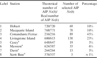
The ionograms are recorded at a sampling rate of 60 min at each station, and so the theoretical number of ionograms to be considered for the analysis is given by the total number of days (DTOT) shown in Table II multiplied by 24. However, the sampling rate sometimes sporadically changes to 30 min, with the result that the real number of Ne(h) analysed can be greater than the theoretical number, and vice versa, because ionosonde observations are occasionally missing and the real number of Ne(h) analysed is less than the theoretical number.
Table III summarizes the theoretical number of AIP Ne(h) for each ionospheric observatory, the real number of AIP Ne(h) analysed, and the number of AIP Ne(h) actually selected and then used as reference profiles.
Table III The theoretical and real ionograms database for each ionospheric observatory is shown in the first column. The subset of ionograms actually employed to carry out the statistical analyses with their corresponding percentages are also shown.

a Located inside the Antarctic Polar Circle.
AIP=Adaptive Ionospheric Profiler.
It is important to point out that the selected AIP Ne(h) are ‘validated’ data in the sense that they are derived from ‘validated’ ionograms, i.e. from ionograms for which the values of foF2 and hmF2 obtained manually by an operator match those given by Autoscala, and for which the restored trace starting from the obtained Ne(h) matches the recorded trace. Some examples of AIP Ne(h) along with the corresponding ionograms from which the AIP profiles were derived are shown in Fig. 2.

Fig. 2 Some examples of ionograms recorded at a. Hobart (Hob), b. Macquarie Island (Mac Isl), c. Comandante Ferraz (Com Ferraz), d. Livingstone Island (Liv Isl), e. Casey (Cas), f. Mawson (Maw), g. Davis (Dav) and h. Scott Base (Scb), along with the corresponding Ne(h) output by Adaptive Ionospheric Profiler (AIP; green traces) and ionograms reconstructed from the AIP profile (red traces), shown for different epochs.
For each ionospheric observatory, the selected AIP profiles were compared with the Ne(h) provided by NeQuick2 operating under two different modes: i) as a climatological model taking as input the F10.7 solar activity index (hereafter, NeQuick2 F10.7) and ii) as an assimilative model ingesting the foF2 and hmF2 measurements obtained from the Ne(h) provided by the AIP (hereafter, NeQuick2 Data Ingestion or NQ-DI). Some examples of these comparisons are shown in Fig. 3.

Fig. 3 Some examples of comparisons between the Adaptive Ionospheric Profiler (AIP) Ne(h) (red plot) and NeQuick2 Ne(h) generated by ingesting bottomside parameters (green plot) and in long-term (yellow plot) prediction mode at a. Hobart (HOB), b. Macquarie Island (MAC), c. Comandante Ferraz (C. FER), d. Livingstone Island (LIV), e. Casey (CAS), f. Mawson (MAW), g. Davis (DAV) and h. Scott Base (SCB), shown for the same epochs and ionospheric observatories as the ionograms depicted in Fig. 2.
For each ionospheric observatory, the selected AIP profiles were also compared to the Ne(h) provided by the climatological IRI2012 model (hereafter, IRI2012 F10.7) and the Ne(h) obtained from the assimilative IRI2012 model (hereafter, IRI2012 Data Ingestion or I-DI). Some examples of these comparisons are shown in Fig. 4.

Fig. 4 Some examples of comparisons between the Adaptive Ionospheric Profiler (AIP) Ne(h) (red plot) and IRI2012 Ne(h) generated by ingesting bottomside parameters (green plot) and in long-term (yellow plot) prediction mode at a. Hobart (HOB), b. Macquarie Island (MAC), c. Comandante Ferraz (C. FER), d. Livingstone Island (LIV), e. Casey (CAS), f. Mawson (MAW), g. Davis (DAV) and h. Scott Base (SCB), shown for the same epochs and ionospheric observatories as the ionograms depicted in Fig. 2.
A visual inspection of a very large number of comparisons, such as those shown in Figs 3 & 4, clearly reveals that the assimilation of autoscaled data, i.e. the foF2 and hmF2 values, is crucially important for achieving more reliable ionospheric modelling.
As a preliminary step, for each ionospheric observatory the AIP profiles selected up to the bottomside and the corresponding Ne(h) modelled by the NQ-DI, NeQuick2 F10.7, I-DI and IRI2012 F10.7 were added up, in order to have a larger number of samples from which to calculate a statistically more significant r.m.s.e. From the five different databases thus obtained, the r.m.s.e. was calculated as follows:
 $$\eqalignno{ & rmse_{{NQ}} {_{\hbox \-}}_{{DI}} \,\,{\equals}\,\,\sqrt {{{\mathop{\sum}\limits_{h\,{\rm min}\,{\equals}\,91km}^{h\,{\rm max\,{\equals}\,}hmF\,{\rm 2}km} {(fp(h)_{{AIP}} } \,{{\minus}}\,fp(h)_{NQ {\hbox \-} DI} )^{2} } \over N}} \cr & rmse_{{NeQuick}} {_{}} _{{2F10.7}} \,{\equals}\,\sqrt {{{\mathop{\sum}\limits_{h\,{\rm min}\,{\equals}\,91km}^{h\,{\rm max\,{\equals}\,}hmF\,{\rm 2}km} {(fp(h)_{{AIP}} } {\,{\minus}}\, fp(h)_{{NeQuick 2F10.7}} )^{2} } \over N}}, $$
 $$\eqalignno{ & rmse_{I} _{_{\hbox \-}} _{{DI}} \,{\equals}\,\sqrt {{{\mathop{\sum}\limits_{h\,{\rm min}\,{\equals}\,91km}^{h\,{\rm max\,{\equals}\,}hmF\,{\rm 2}km} {(fp(h)_{{AIP}} } \,{{\minus}}\,fp(h)_{{{\rm I {\hbox \-} DI}}} )^{2} } \over N}} \cr & rmse_{{IRI}}_{{}} _{{2012F10.7}} \,{\equals}\,\sqrt {{{\mathop{\sum}\limits_{h\,{\rm min}\,{\equals}\,91km}^{h\,{\rm max\,{\equals}\,}hmF\,{\rm 2}km} {(fp(h)_{{AIP}} } \,{{\minus}}\,fp(h)_{{IRI 2012F10.7}} )^{2} } \over N}.} $$
In Eq. (1a) & (1b), N is the total number of samples (fp(h) values), fp(h)AIP, is the reference plasma frequency given by AIP, fp(h)NQ-DI, fp(h)NeQuick2F10.7, fp(h)I-DI and fp(h)IRI2012F10.7 are the plasma frequencies modelled respectively by NQ-DI, NeQuick2 F10.7, I-DI and IRI2012 F10.7 at a definite real height (h).
The r.m.s.e. analysis results are shown in Fig. 5 and demonstrate that the NQ-DI and I-DI models perform better than the NeQuick2 F10.7 and IRI2012 F10.7 models, respectively. Some examples of comparisons between the AIP, NQ-DI and I-DI Ne(h) are shown in Fig. 6. To better highlight a possible dependence of performance on geographical latitude, a direct comparison between the r.m.s.e. values provided by NQ-DI and I-DI is also plotted in Fig. 7 as a function of the geographical latitude of the ionospheric observatories considered in this study. The number of samples on which the r.m.s.e. is calculated for each ionospheric observatory is also plotted as a function of geographical latitude and shown in Fig. 8. Starting from the APC, a marked decrease in the number of samples included in the statistical analysis is observed.

Fig. 5 Root mean square error (r.m.s.e.) for each station, as labelled in Table I, by a. the NeQuick2 Data Ingestion (green dots) and NeQuick2 F10.7 (yellow dots) models, b. the IRI2012 Data Ingestion (blue dots) and IRI2012 F10.7 (yellow dots) models, as a function of geographical latitude. * marks the ionospheric observatories located inside the Antarctic Polar Circle.

Fig. 6 As in Fig. 3, but for the IRI2012 and NeQuick2 Data Ingestion models.

Fig. 7 Trend of root mean square error (r.m.s.e.) obtained by the NeQuick2 Data Ingestion (green dots) and IRI2012 Data Ingestion (blue dots) models as a function of geographical latitude. * marks the ionospheric observatories located inside the Antarctic Polar Circle.

Fig. 8 Number of samples as a function of geographical latitude. * marks the ionospheric observatories located inside the Antarctic Polar Circle.
Discussion
A visual inspection of a very large number of comparisons between the Ne(h) provided by NeQuick2 and IRI2012, when operating both as climatological and assimilative models, shows unequivocally that a better specification of the ionosphere is provided by the NQ-DI and I-DI models (see the examples in Fig. 3 for NeQuick2 and Fig. 4 for IRI2012). This is also quantitatively confirmed when comparing the r.m.s.e. values provided by IRI2012 and NeQuick2 before and after the ingestion of bottomside parameters; in fact, except for Davis (case NeQuick2), the r.m.s.e. are greater when the standard climatological models are considered (see Fig. 5).
This means that: i) the NeQuick2 and IRI2012 models less efficiently represent the real behaviour of the high latitude ionosphere when operating in long-term prediction mode and ii) the best description of the ionospheric environment at southern mid and high latitudes and over the Antarctic area is provided when autoscaled foF2 and hmF2 values are ingested into the NeQuick2 and IRI2012 models. These results again confirm how the data ingestion techniques already investigated in some previous studies (Nava et al. Reference Nava, Radicella and Azpilicueta2011, Pezzopane et al. Reference Pezzopane, Pietrella, Pignatelli, Zolesi and Cander2011, Reference Pezzopane, Pietrella, Pignatelli, Zolesi and Cander2013, Pietrella et al. Reference Pietrella, Pezzopane and Settimi2016, Sabbagh et al. Reference Sabbagh, Scotto and Sgrigna2016) can provide better results than the climatological models.
The r.m.s.e. at Hobart, Macquarie Island, Comandante Ferraz, Livingstone Island and Casey produced by NQ-DI and I-DI are, respectively, 0.68 vs 2.26 MHz, 0.69 vs 1.43 MHz, 1.10 vs 1.20 MHz, 1.08 vs 1.77 MHz and 0.66 vs 1.37 MHz. This means that, up to the APC, including Casey which lies just over the APC, NQ-DI performs far better than I-DI, making r.m.s.e. much smaller than those produced by I-DI. The situation is different when considering the ionospheric observatories of Mawson, Davis and Scott Base, where the r.m.s.e. produced by NQ-DI and I-DI are, respectively, 1.38 vs 1.33 MHz, 2.72 vs 1.91 MHz and 0.93 vs 0.71 MHz. These results reveal that beyond the APC, I-DI performs better than NQ-DI, particularly at Davis and Scott Base, although in the latter case only a small number of available samples were considered.
It is important to note that these results were achieved for a relatively limited ionograms database and for this reason they should be considered as strictly preliminary. One reason for the scarcity of ionograms, as already mentioned, is the extreme complexity of the high latitude ionosphere. This is explained by the fact that, while at mid-latitudes, the main sources of ionization are ultra-violet (UV) and x-ray emissions from the Sun, at high latitudes the Earth’s magnetic field is structured such that, when the north–south direction (Bz) of the interplanetary magnetic field is orientated southwards (Bz<0), the geomagnetic field lines can connect to the outer magnetosphere. When this occurs, solar wind particles, mainly electrons and protons, come directly into the ionosphere and represent an additional source of ionization to the UV and x-rays, considerably complicating the structure of the high latitude ionosphere. The solar wind and the occurrence of a Bz<0 thus play an important role in the dynamics and behaviour of the ionosphere at high latitudes, which can thus be characterized by magneto-ionospheric storms, auroral phenomena, ‘troughs’ of lower ionization at subauroral latitudes, polar cup patches and Sun-aligned arcs. All this makes the morphology of the high latitude ionosphere considerably more complicated and different in general from the morphology of the mid-latitude ionosphere. In particular, polar cup patches are manifested as localized regions of enhanced electron density on spatial scales ranging from 200 to 1000 km horizontally (Moskaleva & Zaalov Reference Moskaleva and Zaalov2013). Other large-scale structural features exhibiting augmented electron density include Sun-aligned arcs, characterized by a dusk–dawn drift (Hunsucker & Hargreaves Reference Hunsucker and Hargreaves2003).
Electron density gradients related to these large-scale high latitude ionospheric inhomogeneities have an important effect on the propagation of high frequency (HF) radio signals. In fact, very large deviations on the direction of arrival of HF radio signals, with bearings up to±100°, have been attributed to the trough at subauroral latitudes (Siddle et al. Reference Siddle, Stocker and Warrington2004a, Reference Siddle, Zaalov, Stocker and Warrington2004b), as well as to the presence of patches and arcs of enhanced electron density (Warrington et al. Reference Warrington, Rogers and Jones1997). Moreover, as also observed at mid-latitudes, electron density inhomogeneities roughen the reflecting surface, increasing the directional spread of signals arriving at the receiver (Bianchi et al. Reference Bianchi, Baskaradas, Pezzopane, Pietrella, Sciacca and Zuccheretti2013). The complexity of the structure and dynamics of the high latitude ionosphere is clearly reflected in ground-based observations based on vertical ionosonde soundings. Ionograms recorded at high latitudes are often rather different from those recorded at mid-latitudes. Due to scattering from large-scale ionospheric irregularities, radio echoes reflected from the F2 layer have a longer duration than the transmitted pulses, which can cause a relatively large spread of signals from the F2 layer, usually referred to as the spread-F phenomenon (Shimazaki Reference Shimazaki1962). Often the spread-F phenomenon is so widespread that it is very difficult, if not impossible, to determine the value of foF2 from the ionogram.
Some examples of these ionograms are shown in Fig. 1. A careful analysis of the geomagnetic activity calculated in terms of ∑Kp (where Kp is the three hourly magnetic planetary index and ∑Kp its sum for one day, for download see http://wdc.kugi.kyoto-u.ac.jp/kp/index.html) revealed that the spread-F event observed in the ionograms recorded on 28 March 2001 at Hobart and Casey, and on 31 March 2001 at Macquarie Island, could be caused by ionospheric irregularities resulting from the presence of obliquely tilted iso-electron density surfaces caused by large-scale wave structures (LSWS) related to the propagation of gravity waves triggered by the geomagnetic activity.
The values for geomagnetic activity expressed in terms of ∑Kp, observed around 27–28 March (see Fig. 9a), are>16, making them compatible with an LSWS occurrence frequency of 25/27 (Testud Reference Testud1970). It is thus highly probable that these disturbed conditions triggered a LSWS, which was responsible for the spread-F phenomena observed at Hobart and Casey on 28 March 2001. On the other hand, the geomagnetic conditions observed in the time interval 28–31 March 2001 (see Fig. 9b), characterized by ∑Kp values always > 16, could have triggered another LSWS and caused the spread-F phenomenon observed at Macquarie Island.

Fig. 9 Geomagnetic activity expressed in terms of ∑Kp a. three days before and three days after 28 March 2001, the day of the ionograms recorded at Hobart at 18h00 UT and Casey at 02h00 UT, b. three days before and three days after 31 March 2001, the day of the ionogram recorded at Macquarie Island at 04h00 UT. The horizontal lines mark the levels of ∑Kp=16, above which the occurrence frequency of large-scale gravity waves reaches 25/27 (Testud Reference Testud1970), and ∑Kp=24, below which magnetic conditions can be considered quiet.
Another important feature of high latitude ionograms is the so-called z-ray (Bowman Reference Bowman1960). This consists of a third trace appearing on ionograms which, like spread-F, can lead to an uncertain determination of foF2 (Scotto Reference Scotto2015). Moreover, the absorption suffered by the electromagnetic waves propagating into the D region, when this is strongly ionized by high energy protons emitted during solar flares (polar cup absorption (PCA) events), gives rise to blank ionograms, thus limiting the number of usable ionograms. Spread-F, z-ray and blank ionograms are therefore expressions of the considerably greater complexity and turbulence of high latitude ionosphere morphology compared to mid-latitudes. Consequently, the automatic recognition of resolved (possibility of routinely scaling foF2 and hmF2) and unresolved (impossibility of routinely scaling foF2 and hmF2 as in the example ionograms shown in Fig. 1) spread-F phenomena, along with the automatic recognition of z-ray (Scotto & Pezzopane Reference Scotto and Pezzopane2012, Scotto Reference Scotto2015) and blank ionograms due to PCA events, constitute the most serious problems to resolve for any automatic scaling software (Reinisch & Huang Reference Reinisch and Huang1983, Reinisch et al. Reference Reinisch, Huang, Galkin, Paznukhov and Kozlov2005). Therefore, the number of reliable ionograms available for this study was greatly limited. This clearly emerges in Fig. 8, where a drastic decrease in the number of data involved in the statistical analysis is observed for the ionospheric observatories located inside the APC. This is directly due to the growing complexity of the ionosphere with increasing latitude for all the reasons described above.
Conclusions
Despite the genuine difficulty of autoscaling ionograms recorded at high latitudes, the authors are confident that by improving the capability of Autoscala to resolve spread-F and z-ray phenomena and reject bad quality ionograms (those that cannot even be scaled manually), while at the same time increasing the number of ionograms on which the AIP can operate, it would certainly be possible to obtain a larger number of reference profiles than those considered in the present investigation. This would enable more significant results from a statistical point of view, as well as a more detailed study on the applicability of NQ-DI and I-DI, exploring their prediction capacity under more diverse geophysical conditions. These studies could help establish which model is more suitable for application, which would be extremely valuable because it would also permit calculation of Ne(h) over the regions surrounding the reference stations using the autoscaled values of foF2 and hmF2.
It would be very worthwhile if these results could be achieved in the future, considering how the automatic scaling of vertical ionograms recorded at mid-latitudes has already proved effective in providing data for improved 3-D real-time specification of the ionosphere. Therefore, improvements for autoscaling ionograms recorded at high latitudes, to provide an ever-greater number of reliable Ne(h), and the applicability of NQ-DI or I-DI in the above-mentioned sense, would represent an interesting approach for achieving nowcasting 3-D electron density mapping and, consequently, space weather forecasting in the ionospheric domain at high latitudes and in polar regions.
Acknowledgements
The authors would like to thank the following scientific institutions: the Ionospheric Prediction Service (Australia) for providing the ionograms database for Hobart, Macquarie Island, Casey, Mawson, Davis and Scott Base, the Istituto Nacional de Pesquisas Espaciais (Brazil) for providing the ionograms for Comandante Ferraz, the Universitat Ramon Lull (Spain) for providing the ionograms for Livingstone Island, and the Progetto Nazionale Ricerche in Antartide for supporting this study. The authors are very grateful to the anonymous referees for their useful comments and suggestions which have greatly contributed to improve the paper.
Author contributions
Marco Pietrella carried out the preliminary study aimed at selecting only the AIP electron density profiles considered to be reliable, he then rearranged the results provided by the other authors and drafted the manuscript. Bruno Nava suitably modified the NeQuick2 model to run as both a climatological and assimilative model, providing comparisons with the AIP electron density profiles. Michael Pezzopane converted the raw ionograms provided by the CADI ionosonde into the RDF format, which is ingested by Autoscala. Yenca Migoya Oruè suitably modified the IRI2012 model to run as both a climatological and assimilative model, providing comparisons with the AIP electron density profiles. Alessandro Ippolito and Carlo Scotto participated in the selection of the AIP electron density profiles, converted ionograms in different formats into the RDF format and adjusted Autoscala for the different ionospheric stations. All the authors actively participated in the discussion of the results and validation of the electron density profiles, as well as reading and approving the final manuscript.