


1. Introduction
Owing to recent advances in manufacturing technologies, metal foams have become commercially available (Calmidi & Mahajan Reference Calmidi and Mahajan1999, Reference Calmidi and Mahajan2000; Dukhan Reference Dukhan2013). Their main features are high specific surface, high thermal conductivity and comparatively high permeability. Thus, metal foams may well be used as efficient heat exchangers, since they exhibit high interstitial heat transfer between the metal and passing fluid, with a moderate pressure drop.
Nanofluids, on the other hand, have attracted extensive attention for the past decade, in view of their great potential as high-energy carriers resulting from their promising feature of high effective thermal conductivity (e.g. Lee & Choi Reference Lee and Choi1996; Pak & Cho Reference Pak and Cho1998; Lee et al. Reference Lee, Choi, Li and Eastman1999; Xuan & Roetzel Reference Xuan and Roetzel2000; Chien & Chuang Reference Chien and Chuang2007; Heris, Esfahany & Etemad Reference Heris, Esfahany and Etemad2007; Yang, Li & Nakayama Reference Yang, Li and Nakayama2013a ). Hence, it is thought that nanofluid-saturated metal foams, being the combination of metal foams and nanofluids, will lead to a new generation of high-performance heat exchangers.
Sakai, Li & Nakayama (Reference Sakai, Li and Nakayama2014) rigorously derived a set of volume-averaged transport equations appropriate for convection in nanofluid-saturated metal foams. However, they assumed local thermal equilibrium between the fluid and metal phases, in which the volume-averaged fluid temperature is assumed to be equal to the metal temperature. In reality, the local thermal equilibrium assumption may fail, since the thermal conductivity of the metal conducting heat from the wall is much higher than that of the nanofluid.
Kuwahara et al. (Reference Kuwahara, Yang, Ando and Nakayama2011) obtained a set of exact solutions for the case of forced convection in a channel filled with a fluid-saturated metal foam, and demonstrated that forced convection in a channel subject to constant wall heat flux must be treated by using a thermal non-equilibrium model, since the fluid and solid phases within the channel are never in thermal equilibrium. This work was followed by that of Yang, Ando & Nakayama (Reference Yang, Ando and Nakayama2011), who also compared the set of exact solutions based on local thermal equilibrium against those based on local thermal non-equilibrium models for the case of tube flows, and concluded that substantial errors result from the assumption of local thermal equilibrium for the case of constant heat flux.
Thus, the local thermal equilibrium assumption should be discarded, and a local thermal non-equilibrium model must be introduced with an interstitial heat transfer model between the nanofluid and metal phases.
Another important feature associated with nanofluid-saturated metal foams may be mechanical dispersion (Yang, Liu & Nakayama Reference Yang, Liu and Nakayama2009; Yang & Nakayama Reference Yang and Nakayama2010). Mechanical dispersion in heat transfer resulting from porous matrices is termed ‘thermal dispersion’, whereas, in this study, mechanical dispersion in nanoparticle transport may be called ‘nanoparticle mechanical dispersion’, i.e. macroscopic dispersion resulting from porous matrices. (This should not be confused with ‘nanoparticle dispersion’, meaning particles dispersed in the base fluid, i.e. microscopic dispersion.)
In this study, we shall derive an appropriate set of volume-averaged transport equations for convection in nanofluid-saturated metal foams, using a volume-averaging theory and allowing the nanofluid temperature and the metal temperature to differ from each other, i.e. local thermal non-equilibrium model. The microscopic transport equations based on the Buongiorno model (Buongiorno Reference Buongiorno2006) for convective heat transfer in nanofluids are modified so as to fully account for the effects of nanoparticle volume fraction distributions on the continuity, momentum and energy equations, and then are integrated within a local averaging volume to obtain an appropriate set of governing equations in terms of volume-averaged dependent variables (Cheng Reference Cheng1978; Quintard & Whitaker Reference Quintard and Whitaker1993; Nakayama Reference Nakayama1995; Quintard & Whitaker Reference Quintard and Whitaker1995). Non-zero terms associated with interfacial surface integrals (Nakayama, Kuwahara & Hayashi Reference Nakayama, Kuwahara and Hayashi2004) and averages of spatial deviations are subsequently modelled mathematically using the volume-averaged dependent variables.
A pore-scale analysis will be conducted to deduce possible functional forms for describing thermal dispersion in a nanofluid-saturated metal foam. Moreover, nanoparticle mechanical dispersion (i.e. macroscopic dispersion resulting from porous matrices) will be focused upon for the first time, and will be modelled mathematically, considering a pore-scale conduit. It will be analytically shown that the longitudinal particle mechanical dispersion works either to suppress or to enhance effective diffusion depending on the sign of the local phase temperature difference, while the transverse counterpart is insignificant and therefore can be neglected. Furthermore, heat transfer performance evaluation under equal pumping power will be made for the case of forced convective heat transfer in a nanofluid-saturated metal foam. We shall demonstrate that an unconventionally high level of the heat transfer rate (about 80 times more than the case of base fluid convection without a metal foam) is attainable by combining a metal foam with a nanofluid.
2. Modified Buongiorno equations for nanofluids
Buongiorno (Reference Buongiorno2006) assumed incompressible flow, no chemical reactions, negligible external forces, dilute mixture, negligible viscous dissipation, negligible radiative heat transfer, and local thermal equilibrium between nanoparticles and base fluid. Local thermal equilibrium between the nanoparticles and the base fluid is obvious since the size of the nanoparticles is so small that nanoparticle temperature changes instantly and coincides with that of the surrounding base fluid. Following Yang et al. (Reference Yang, Li, Sano, Mochizuki and Nakayama2013b ), the two-component mixture model proposed by Buongiorno may be modified to allow nanofluid density variation in mass, momentum and energy conservations as
 $$\begin{eqnarray}\displaystyle & \displaystyle \frac{\partial {\it\rho}u_{j}}{\partial x_{j}}=0, & \displaystyle\end{eqnarray}$$
 $$\begin{eqnarray}\displaystyle & \displaystyle \frac{\partial {\it\rho}u_{i}}{\partial t}+\frac{\partial {\it\rho}u_{j}u_{i}}{\partial x_{j}}=-\frac{\partial p}{\partial x_{i}}+\frac{\partial }{\partial x_{j}}{\it\mu}\left(\frac{\partial u_{i}}{\partial x_{j}}+\frac{\partial u_{j}}{\partial x_{i}}\right), & \displaystyle\end{eqnarray}$$
 $$\begin{eqnarray}\displaystyle & \displaystyle c\left(\frac{\partial {\it\rho}T}{\partial t}+\frac{\partial {\it\rho}u_{j}T}{\partial x_{j}}\right)=\frac{\partial }{\partial x_{j}}\left(k\frac{\partial T}{\partial x_{j}}\right), & \displaystyle\end{eqnarray}$$
 $$\begin{eqnarray}\displaystyle & \displaystyle {\it\rho}_{p}\left(\frac{\partial {\it\phi}}{\partial t}+\frac{\partial u_{j}{\it\phi}}{\partial x_{j}}\right)=\frac{\partial }{\partial x_{j}}\left({\it\rho}_{p}D_{B}\frac{\partial {\it\phi}}{\partial x_{j}}+\frac{{\it\rho}_{p}D_{T}}{T}\frac{\partial T}{\partial x_{j}}\right), & \displaystyle\end{eqnarray}$$
 ${\it\rho},~c,~{\it\mu}$
and
${\it\rho},~c,~{\it\mu}$
and
 $k$
are the density, heat capacity, viscosity and thermal conductivity of the nanofluid, which depend on the nanoparticle volume fraction
$k$
are the density, heat capacity, viscosity and thermal conductivity of the nanofluid, which depend on the nanoparticle volume fraction
 ${\it\phi}$
as
${\it\phi}$
as  $$\begin{eqnarray}\displaystyle & \displaystyle {\it\rho}={\it\phi}{\it\rho}_{p}+(1-{\it\phi}){\it\rho}_{bf}, & \displaystyle\end{eqnarray}$$
 $$\begin{eqnarray}\displaystyle & \displaystyle c=[{\it\phi}{\it\rho}_{p}c_{p}+(1-{\it\phi}){\it\rho}_{bf}c_{bf}]/{\it\rho}, & \displaystyle\end{eqnarray}$$
 $$\begin{eqnarray}\displaystyle & \displaystyle {\it\mu}={\it\mu}_{bf}(1+a_{{\it\mu}}{\it\phi}+b_{{\it\mu}}{\it\phi}^{2})={\it\mu}_{bf}(1+7.3{\it\phi}+123{\it\phi}^{2}), & \displaystyle\end{eqnarray}$$
 $$\begin{eqnarray}\displaystyle & \displaystyle k=k_{bf}(1+a_{k}{\it\phi}+b_{k}{\it\phi}^{2})=k_{bf}(1+2.72{\it\phi}+4.97{\it\phi}^{2}). & \displaystyle\end{eqnarray}$$
 $$\begin{eqnarray}\displaystyle D_{B}=\frac{k_{BO}T}{3{\rm\pi}{\it\mu}_{bf}d_{p}} & & \displaystyle\end{eqnarray}$$
and
 $$\begin{eqnarray}\displaystyle D_{T}=0.26\frac{k_{bf}}{2k_{bf}+k_{p}}\frac{{\it\mu}_{bf}}{{\it\rho}_{bf}}{\it\phi}, & & \displaystyle\end{eqnarray}$$
respectively. The nanofluid thermophysical properties such as
 ${\it\mu}$
and
${\it\mu}$
and
 $k$
are considered as given functions of
$k$
are considered as given functions of
 ${\it\phi}$
. Equations (2.5c
) and (2.5d
) are what appear to be the most reliable correlations proposed by Maiga et al. (Reference Maiga, Palm, Nguyen, Roy and Galanis2005), where the subscripts
${\it\phi}$
. Equations (2.5c
) and (2.5d
) are what appear to be the most reliable correlations proposed by Maiga et al. (Reference Maiga, Palm, Nguyen, Roy and Galanis2005), where the subscripts
 $p$
and
$p$
and
 $bf$
refer to nanoparticle and base fluid, respectively. Moreover,
$bf$
refer to nanoparticle and base fluid, respectively. Moreover,
 $k_{BO}$
is the Boltzmann constant and
$k_{BO}$
is the Boltzmann constant and
 $d_{p}$
is the nanoparticle diameter, which can be anywhere of the order of 1–100 nm. As for the temperature dependence of thermophysical properties, Li & Nakayama (Reference Li and Nakayama2015) investigated the effect of temperature-dependent thermophysical properties on convective heat transfer rates. They found that variations of base fluid properties due to temperature variation are small enough to be neglected compared with the effects of nanoparticle volume fraction and temperature.
$d_{p}$
is the nanoparticle diameter, which can be anywhere of the order of 1–100 nm. As for the temperature dependence of thermophysical properties, Li & Nakayama (Reference Li and Nakayama2015) investigated the effect of temperature-dependent thermophysical properties on convective heat transfer rates. They found that variations of base fluid properties due to temperature variation are small enough to be neglected compared with the effects of nanoparticle volume fraction and temperature.
Many, including Bianco et al. (Reference Bianco, Chiacchio, Manca and Nardini2009), have found that the two-component mixture model is quite adequate for describing nanofluid heat transfer, as supported by Buongiorno (Reference Buongiorno2006) using a magnitudes analysis. The energy equation (2.3) appears to be identical to that of a pure fluid, except that all properties are functions of
 ${\it\phi}$
. It should be noted that the nanoparticle continuity equation (2.4) must be treated simultaneously with (2.1)–(2.3) for the other dependent variables, since the thermophysical properties strongly depend on the spatial distribution of
${\it\phi}$
. It should be noted that the nanoparticle continuity equation (2.4) must be treated simultaneously with (2.1)–(2.3) for the other dependent variables, since the thermophysical properties strongly depend on the spatial distribution of
 ${\it\phi}$
. Most previous researchers neglected the spatial variations of thermophysical properties, including Brownian and thermophoretic diffusion coefficients. Such analytical treatments could result in substantial errors, as discussed in Yang et al. (Reference Yang, Li, Sano, Mochizuki and Nakayama2013b
). In this study, all these variations will be considered.
${\it\phi}$
. Most previous researchers neglected the spatial variations of thermophysical properties, including Brownian and thermophoretic diffusion coefficients. Such analytical treatments could result in substantial errors, as discussed in Yang et al. (Reference Yang, Li, Sano, Mochizuki and Nakayama2013b
). In this study, all these variations will be considered.

Figure 1. The averaging volume in a nanofluid-saturated metal foam. The averaging volume is smaller than the macroscopic characteristic scale but larger than the pore scale.
3. Volume-averaging theory
A volume-averaging procedure may be used to derive a complete set of macroscopic governing equations for convection within a nanofluid-saturated metal foam. Let us consider a local averaging volume
 $V$
in a nanofluid-saturated metal foam, as shown in figure 1, whose length scale
$V$
in a nanofluid-saturated metal foam, as shown in figure 1, whose length scale
 $V^{1/3}$
is much smaller than the macroscopic characteristic length, but, at the same time, much greater than the microscopic characteristic length (see e.g. Cheng Reference Cheng1978; Quintard & Whitaker Reference Quintard and Whitaker1993, Reference Quintard and Whitaker1995; Nakayama Reference Nakayama1995). Under this condition, the volume average of a certain variable
$V^{1/3}$
is much smaller than the macroscopic characteristic length, but, at the same time, much greater than the microscopic characteristic length (see e.g. Cheng Reference Cheng1978; Quintard & Whitaker Reference Quintard and Whitaker1993, Reference Quintard and Whitaker1995; Nakayama Reference Nakayama1995). Under this condition, the volume average of a certain variable
 ${\it\varphi}$
is defined as
${\it\varphi}$
is defined as
 $$\begin{eqnarray}\displaystyle \langle {\it\varphi}\rangle =\frac{1}{V}\int _{V_{f}}{\it\varphi}\text{d}V. & & \displaystyle\end{eqnarray}$$
Another average, namely, the intrinsic average, is given by
 $$\begin{eqnarray}\displaystyle \langle {\it\varphi}\rangle ^{\,f}=\frac{1}{V_{f}}\int _{V_{f}}{\it\varphi}\text{d}V & & \displaystyle\end{eqnarray}$$
where
 $V_{f}$
is a volume space that the nanofluid occupies. Obviously, the two averages are related as
$V_{f}$
is a volume space that the nanofluid occupies. Obviously, the two averages are related as
 $\langle {\it\varphi}\rangle ={\it\varepsilon}\langle {\it\varphi}\rangle ^{\,f}$
, where
$\langle {\it\varphi}\rangle ={\it\varepsilon}\langle {\it\varphi}\rangle ^{\,f}$
, where
 ${\it\varepsilon}=V_{f}/V$
is the porosity, namely, the local volume fraction of the nanofluid phase. We decompose a variable into its intrinsic average and the spatial deviation from it:
${\it\varepsilon}=V_{f}/V$
is the porosity, namely, the local volume fraction of the nanofluid phase. We decompose a variable into its intrinsic average and the spatial deviation from it:
 $$\begin{eqnarray}\displaystyle {\it\varphi}=\langle {\it\varphi}\rangle ^{\,f}+\tilde{{\it\varphi}}. & & \displaystyle\end{eqnarray}$$
All dependent variables in the microscopic governing equations for the nanofluid and metal phases will be decomposed in this manner. We shall utilize the following spatial average relationships:
 $$\begin{eqnarray}\displaystyle \langle {\it\varphi}_{1}{\it\varphi}_{2}\rangle ^{\,f}=\langle {\it\varphi}_{1}\rangle ^{\,f}\langle {\it\varphi}_{2}\rangle ^{\,f}+\langle \tilde{{\it\varphi}}_{1}\tilde{{\it\varphi}}_{2}\rangle ^{\,f} & & \displaystyle\end{eqnarray}$$
 $$\begin{eqnarray}\left\langle \frac{\partial {\it\varphi}}{\partial x_{i}}\right\rangle =\frac{\partial \langle {\it\varphi}\rangle }{\partial x_{i}}+\frac{1}{V}\int _{A_{int}}{\it\varphi}n_{i}\text{d}A\quad \text{or}\quad \left\langle \frac{\partial {\it\varphi}}{\partial x_{i}}\right\rangle ^{f}=\frac{1}{{\it\varepsilon}}\frac{\partial {\it\varepsilon}\langle {\it\varphi}\rangle ^{\,f}}{\partial x_{i}}+\frac{1}{V_{f}}\int _{A_{int}}{\it\varphi}n_{i}\text{d}A\end{eqnarray}$$
and
 $$\begin{eqnarray}\displaystyle \left\langle \frac{\partial {\it\varphi}}{\partial t}\right\rangle =\frac{\partial \langle {\it\varphi}\rangle }{\partial t}. & & \displaystyle\end{eqnarray}$$
Here
 $A_{int}$
represents the interfaces between fluid and solid matrix within a local averaging volume. Note that
$A_{int}$
represents the interfaces between fluid and solid matrix within a local averaging volume. Note that
 $n_{i}$
is the unit vector pointing outwards from the nanofluid side to the solid side. All dependent variables for nanofluid and metal phases are decomposed according to (3.2). Then, the microscopic equations (2.1)–(2.4) are integrated over a local averaging volume, exploiting the foregoing spatial average relationships. The set of macroscopic governing equations thus obtained for nanofluid and metal phases in a nanofluid-saturated metal foam with uniform porosity
$n_{i}$
is the unit vector pointing outwards from the nanofluid side to the solid side. All dependent variables for nanofluid and metal phases are decomposed according to (3.2). Then, the microscopic equations (2.1)–(2.4) are integrated over a local averaging volume, exploiting the foregoing spatial average relationships. The set of macroscopic governing equations thus obtained for nanofluid and metal phases in a nanofluid-saturated metal foam with uniform porosity
 ${\it\varepsilon}$
may be given as follows:
${\it\varepsilon}$
may be given as follows:
 $$\begin{eqnarray}\displaystyle & & \displaystyle \displaystyle \frac{\partial {\it\rho}\langle u_{j}\rangle ^{\,f}}{\partial x_{j}}+\frac{1}{V_{f}}\int _{A_{int}}{\it\rho}u_{j}n_{j}\text{d}A=0,\end{eqnarray}$$
 $$\begin{eqnarray}\displaystyle & & \displaystyle \displaystyle \frac{\partial {\it\rho}\langle u_{i}\rangle ^{\,f}}{\partial t}+\frac{\partial {\it\rho}\langle u_{j}\rangle ^{\,f}\langle u_{i}\rangle ^{\,f}}{\partial x_{j}}\nonumber\\ \displaystyle & & \displaystyle \quad =-\frac{\partial \langle p\rangle ^{\,f}}{\partial x_{i}}+\frac{\partial }{\partial x_{j}}\left({\it\mu}\left(\frac{\partial \langle u_{i}\rangle ^{\,f}}{\partial x_{j}}+\frac{\partial \langle u_{j}\rangle ^{\,f}}{\partial x_{i}}\right)+\frac{{\it\mu}}{V_{f}}\int _{A_{int}}(u_{i}n_{j}+u_{j}n_{i})\text{d}A-{\it\rho}\langle \tilde{u} _{i}\tilde{u} _{j}\rangle ^{\,f}\right)\nonumber\\ \displaystyle & & \displaystyle \qquad +\,\frac{1}{V_{f}}\int _{A_{int}}\left({\it\mu}\left(\frac{\partial u_{i}}{\partial x_{j}}+\frac{\partial u_{j}}{\partial x_{i}}\right)-p{\it\delta}_{ij}\right)n_{j}\text{d}A-\frac{1}{V_{f}}\int _{A_{int}}{\it\rho}u_{j}u_{i}n_{j}\text{d}A,\end{eqnarray}$$
 $$\begin{eqnarray}\displaystyle & & \displaystyle \displaystyle {\it\varepsilon}c\left(\frac{\partial {\it\rho}\langle T\rangle ^{\,f}}{\partial t}+\frac{\partial {\it\rho}\langle u_{j}\rangle ^{\,f}\langle T\rangle ^{\,f}}{\partial x_{j}}\right)\nonumber\\ \displaystyle & & \displaystyle \quad =\frac{\partial }{\partial x_{j}}\left({\it\varepsilon}k\frac{\partial \langle T\rangle ^{\,f}}{\partial x_{j}}+\frac{k}{V}\int _{A_{int}}Tn_{j}\text{d}A-{\it\varepsilon}{\it\rho}c\langle \tilde{T}\tilde{u} _{j}\rangle ^{\,f}\right)\nonumber\\ \displaystyle & & \displaystyle \qquad +\,\frac{1}{V}\int _{A_{int}}k\frac{\partial T}{\partial x_{j}}n_{j}\text{d}A-\frac{c}{V}\int _{A_{int}}{\it\rho}Tu_{j}n_{j}\text{d}A,\end{eqnarray}$$
 $$\begin{eqnarray}\displaystyle & & \displaystyle \displaystyle (1-{\it\varepsilon})c_{s}\frac{\partial \langle T\rangle ^{s}}{\partial t}=\frac{\partial }{\partial x_{j}}\left((1-{\it\varepsilon})k_{s}\frac{\partial \langle T\rangle ^{s}}{\partial x_{j}}-\frac{k_{s}}{V}\int _{A_{int}}Tn_{j}\text{d}A\right)-\frac{1}{V}\int _{A_{int}}k_{s}\frac{\partial T}{\partial x_{j}}n_{j}\text{d}A\end{eqnarray}$$
 $$\begin{eqnarray}\displaystyle & & \displaystyle \displaystyle \frac{\partial \langle {\it\phi}\rangle ^{\,f}}{\partial t}+\frac{\partial \langle u_{j}\rangle ^{\,f}\langle {\it\phi}\rangle ^{\,f}}{\partial x_{j}}\nonumber\\ \displaystyle & & \displaystyle \quad =\frac{\partial }{\partial x_{j}}\left(D_{B}\frac{\partial \langle {\it\phi}\rangle ^{\,f}}{\partial x_{j}}+\frac{D_{T}}{\langle T\rangle ^{\,f}}\frac{\partial \langle T\rangle ^{\,f}}{\partial x_{j}}+\frac{D_{B}}{V_{f}}\int _{A_{int}}{\it\phi}n_{j}\text{d}A+\frac{D_{T}}{V_{f}\langle T\rangle ^{\,f}}\int _{A_{int}}Tn_{j}\text{d}A-\langle \tilde{{\it\phi}}\tilde{u} _{j}\rangle ^{\,f}\right)\nonumber\\ \displaystyle & & \displaystyle \qquad +\,\frac{1}{V_{f}}\int _{A_{int}}\left(D_{B}\frac{\partial {\it\phi}}{\partial x_{j}}+\frac{D_{T}}{\langle T\rangle ^{f}}\frac{\partial T}{\partial x_{j}}\right)n_{j}\text{d}A-\frac{1}{V_{f}}\int _{A_{int}}u_{j}{\it\phi}n_{j}\text{d}A.\end{eqnarray}$$
 $$\begin{eqnarray}u_{j}=\mathbf{0}\quad \text{and}\quad \left(D_{B}\frac{\partial {\it\phi}}{\partial x_{j}}+\frac{D_{T}}{T}\frac{\partial T}{\partial x_{j}}\right)n_{j}=0.\end{eqnarray}$$
Thus, many surface integral terms vanish and the equations reduce to
 $$\begin{eqnarray}\displaystyle & & \displaystyle \displaystyle \frac{\partial {\it\rho}\langle u_{j}\rangle ^{\,f}}{\partial x_{j}}=0,\end{eqnarray}$$
 $$\begin{eqnarray}\displaystyle & & \displaystyle \displaystyle \frac{\partial {\it\rho}\langle u_{i}\rangle ^{\,f}}{\partial t}+\frac{\partial {\it\rho}\langle u_{j}\rangle ^{\,f}\langle u_{i}\rangle ^{\,f}}{\partial x_{j}}\nonumber\\ \displaystyle & & \displaystyle \quad =-\frac{\partial \langle p\rangle ^{\,f}}{\partial x_{i}}+\frac{\partial }{\partial x_{j}}\left({\it\mu}\left(\frac{\partial \langle u_{i}\rangle ^{f}}{\partial x_{j}}+\frac{\partial \langle u_{j}\rangle ^{f}}{\partial x_{i}}\right)-{\it\rho}\langle \tilde{u} _{i}\tilde{u} _{j}\rangle ^{\,f}\right)\nonumber\\ \displaystyle & & \displaystyle \qquad +\,\frac{1}{V_{f}}\int _{A_{b_{int}}}\left({\it\mu}\left(\frac{\partial u_{i}}{\partial x_{j}}+\frac{\partial u_{j}}{\partial x_{i}}\right)-p{\it\delta}_{ij}\right)n_{j}\text{d}A,\end{eqnarray}$$
 $$\begin{eqnarray}\displaystyle & & \displaystyle \displaystyle {\it\varepsilon}c\left(\frac{\partial {\it\rho}\langle T\rangle ^{f}}{\partial t}+\frac{\partial {\it\rho}\langle u_{j}\rangle ^{f}\langle T\rangle ^{\,f}}{\partial x_{j}}\right)\nonumber\\ \displaystyle & & \displaystyle \quad =\frac{\partial }{\partial x_{j}}\left({\it\varepsilon}k\frac{\partial \langle T\rangle ^{\,f}}{\partial x_{j}}+\frac{k}{V}\int _{A_{int}}Tn_{j}\text{d}A-{\it\varepsilon}{\it\rho}c\langle \tilde{T}\tilde{u} _{j}\rangle ^{\,f}\right)+\frac{1}{V}\int _{A_{int}}k\frac{\partial T}{\partial x_{j}}n_{j}\text{d}A,\end{eqnarray}$$
 $$\begin{eqnarray}\displaystyle & & \displaystyle \displaystyle (1-{\it\varepsilon})c_{s}\frac{\partial {\it\rho}\langle T\rangle ^{s}}{\partial t}=\frac{\partial }{\partial x_{j}}\left((1-{\it\varepsilon})k_{s}\frac{\partial \langle T\rangle ^{s}}{\partial x_{j}}-\frac{k_{s}}{V}\int _{A_{int}}Tn_{j}\text{d}A\right)-\frac{1}{V}\int _{A_{int}}k\frac{\partial T}{\partial x_{j}}n_{j}\text{d}A,\end{eqnarray}$$
 $$\begin{eqnarray}\displaystyle & & \displaystyle \displaystyle {\it\varepsilon}\left(\frac{\partial \langle {\it\phi}\rangle ^{\,f}}{\partial t}+\frac{\partial \langle u_{j}\rangle ^{\,f}\langle {\it\phi}\rangle ^{\,f}}{\partial x_{j}}\right)\nonumber\\ \displaystyle & & \displaystyle \quad =\frac{\partial }{\partial x_{j}}\left({\it\varepsilon}D_{B}\frac{\partial \langle {\it\phi}\rangle ^{\,f}}{\partial x_{j}}+\frac{{\it\varepsilon}D_{T}}{\langle T\rangle ^{\,f}}\frac{\partial \langle T\rangle ^{\,f}}{\partial x_{j}}+\frac{D_{B}}{V}\int _{A_{int}}{\it\phi}n_{j}\text{d}A+\frac{D_{T}}{V\langle T\rangle ^{\,f}}\int _{A_{int}}Tn_{j}\text{d}A-{\it\varepsilon}\langle \tilde{{\it\phi}}\tilde{u} _{j}\rangle ^{\,f}\right).\nonumber\\ \displaystyle & & \displaystyle\end{eqnarray}$$
In the previous equations, the correlations associated with deviations,
 $-{\it\rho}\langle \tilde{u} _{i}\tilde{u} _{j}\rangle ^{\,f}$
,
$-{\it\rho}\langle \tilde{u} _{i}\tilde{u} _{j}\rangle ^{\,f}$
,
 $-{\it\varepsilon}{\it\rho}c\langle \tilde{T}\tilde{u} _{j}\rangle ^{\,f}$
and
$-{\it\varepsilon}{\it\rho}c\langle \tilde{T}\tilde{u} _{j}\rangle ^{\,f}$
and
 $-{\it\varepsilon}\langle \tilde{{\it\phi}}\tilde{u} _{j}\rangle ^{\,f}$
, correspond to mechanical dispersion terms, whereas the surface integral terms,
$-{\it\varepsilon}\langle \tilde{{\it\phi}}\tilde{u} _{j}\rangle ^{\,f}$
, correspond to mechanical dispersion terms, whereas the surface integral terms,
 $(k/V)\int _{A_{int}}\!Tn_{j}\text{d}A$
,
$(k/V)\int _{A_{int}}\!Tn_{j}\text{d}A$
,
 $(D_{B}/V)\int _{A_{int}}\!{\it\phi}n_{j}\text{d}A$
and
$(D_{B}/V)\int _{A_{int}}\!{\it\phi}n_{j}\text{d}A$
and
 $(D_{T}/(V\langle T\rangle ^{\,f}))\int _{A_{int}}\!Tn_{j}\text{d}A$
, correspond to the tortuosity terms.
$(D_{T}/(V\langle T\rangle ^{\,f}))\int _{A_{int}}\!Tn_{j}\text{d}A$
, correspond to the tortuosity terms.
4. Mathematical modelling
As usual, the Forchheimer-extended Darcy law is introduced to describe the internal flow resistance:
 $$\begin{eqnarray}\displaystyle \frac{1}{V_{f}}\!\int _{A_{int}}\!\!\left({\it\mu}\!\left(\frac{\partial u_{i}}{\partial x_{j}}+\frac{\partial u_{j}}{\partial x_{i}}\right)\!-p{\it\delta}_{ij}\right)n_{j}\text{d}A\,\frac{\partial }{\partial x}{\it\rho}\langle \tilde{u} _{i}\tilde{u} _{j}\rangle ^{\,f}=-\frac{{\it\varepsilon}{\it\mu}}{K}\langle u_{j}\rangle ^{\,f}-{\it\rho}{\it\varepsilon}^{2}b\sqrt{\langle u_{k}\rangle ^{\,f}\langle u_{k}\rangle ^{f}}\langle u_{j}\rangle ^{\,f}, & & \displaystyle \nonumber\\ \displaystyle & & \displaystyle\end{eqnarray}$$
while tortuosity in nanoparticle volume fraction transport is neglected since
 $$\begin{eqnarray}\displaystyle \frac{D_{B}}{V_{f}}\int _{A_{int}}{\it\phi}n_{j}\text{d}A\cong \frac{D_{B}}{V_{f}}{\it\phi}\int _{A_{int}}n_{j}\text{d}A=\mathbf{0}. & & \displaystyle\end{eqnarray}$$
The tortuosity terms in the two energy equations may be modelled by introducing the Yang–Nakayama effective porosity
 ${\it\varepsilon}^{\ast }$
(Yang & Nakayama Reference Yang and Nakayama2010; Kuwahara et al.
Reference Kuwahara, Yang, Ando and Nakayama2011) as
${\it\varepsilon}^{\ast }$
(Yang & Nakayama Reference Yang and Nakayama2010; Kuwahara et al.
Reference Kuwahara, Yang, Ando and Nakayama2011) as
 $$\begin{eqnarray}\displaystyle & \displaystyle {\it\varepsilon}k\frac{\partial \langle T\rangle ^{\,f}}{\partial x_{j}}+\frac{k}{V}\int _{A_{int}}Tn_{j}\text{d}A={\it\varepsilon}^{\ast }k\frac{\partial \langle T\rangle ^{\,f}}{\partial x_{j}}, & \displaystyle\end{eqnarray}$$
 $$\begin{eqnarray}\displaystyle & \displaystyle (1-{\it\varepsilon})k_{s}\frac{\partial \langle T\rangle ^{s}}{\partial x_{j}}-\frac{k_{s}}{V}\int _{A_{int}}Tn_{j}\text{d}A=(1-{\it\varepsilon}^{\ast })k_{s}\frac{\partial \langle T\rangle ^{s}}{\partial x_{j}}, & \displaystyle\end{eqnarray}$$
 $$\begin{eqnarray}\displaystyle {\it\varepsilon}^{\ast }=\frac{k_{s}-k_{stag}}{k_{s}-k_{f}} & & \displaystyle\end{eqnarray}$$
where
 $k_{stag}$
is the stagnant thermal conductivity of the saturated porous medium, which can readily be measured using a standard method. However, for the cases of high-conductivity porous media, such as metal foams, satisfying the condition
$k_{stag}$
is the stagnant thermal conductivity of the saturated porous medium, which can readily be measured using a standard method. However, for the cases of high-conductivity porous media, such as metal foams, satisfying the condition
 $k_{s}/k\gg 3/(1-{\it\varepsilon})$
, there is no need to measure the stagnant thermal conductivity of the saturated porous medium, since the effective porosity may be approximated well by
$k_{s}/k\gg 3/(1-{\it\varepsilon})$
, there is no need to measure the stagnant thermal conductivity of the saturated porous medium, since the effective porosity may be approximated well by
 $$\begin{eqnarray}\displaystyle {\it\varepsilon}^{\ast }=\frac{2+{\it\varepsilon}}{3} & & \displaystyle\end{eqnarray}$$
according to Yang & Nakayama (Reference Yang and Nakayama2010). For example, in the case of the combination of aluminium foam and water, we typically have
 $k_{s}/k\cong 330$
and
$k_{s}/k\cong 330$
and
 ${\it\varepsilon}=0.90$
. Thus,
${\it\varepsilon}=0.90$
. Thus,
 $k_{s}/k\gg 3/(1-{\it\varepsilon})$
is satisfied such that
$k_{s}/k\gg 3/(1-{\it\varepsilon})$
is satisfied such that
 ${\it\varepsilon}^{\ast }=(2+0.9)/3=0.97$
. Furthermore, Newton’s cooling law may be adopted for the interstitial heat transfer between the nanofluid phase and the metal foam as
${\it\varepsilon}^{\ast }=(2+0.9)/3=0.97$
. Furthermore, Newton’s cooling law may be adopted for the interstitial heat transfer between the nanofluid phase and the metal foam as
 $$\begin{eqnarray}\frac{1}{V}\int _{A_{int}}k\frac{\partial T}{\partial x_{j}}n_{j}\text{d}A=h_{v}(\langle T\rangle ^{s}-\langle T\rangle ^{\,f}),\end{eqnarray}$$
where
 $h_{v}$
is the volumetric interstitial heat transfer coefficient. Upon implementing the foregoing mathematical models, the equations reduce to
$h_{v}$
is the volumetric interstitial heat transfer coefficient. Upon implementing the foregoing mathematical models, the equations reduce to
 $$\begin{eqnarray}\displaystyle \frac{\partial {\it\rho}\langle u_{j}\rangle }{\partial x_{j}}=0, & & \displaystyle\end{eqnarray}$$
 $$\begin{eqnarray}\displaystyle \frac{1}{{\it\varepsilon}}\frac{\partial {\it\rho}\langle u_{i}\rangle }{\partial t}+\frac{1}{{\it\varepsilon}^{2}}\frac{\partial {\it\rho}\langle u_{j}\rangle \langle u_{i}\rangle }{\partial x_{j}}=-\frac{\partial \langle p\rangle ^{f}}{\partial x_{i}}+\frac{\partial }{\partial x_{j}}\left(\frac{{\it\mu}}{{\it\varepsilon}}\frac{\partial \langle u_{i}\rangle }{\partial x_{j}}\right)-\frac{{\it\mu}}{K}\langle u_{i}\rangle -{\it\rho}b\sqrt{\langle u_{k}\rangle \langle u_{k}\rangle }\langle u_{i}\rangle , & & \displaystyle \nonumber\\ \displaystyle & & \displaystyle\end{eqnarray}$$
 $$\begin{eqnarray}\displaystyle & \displaystyle {\it\varepsilon}c\frac{\partial {\it\rho}\langle T\rangle ^{\,f}}{\partial t}+c\frac{\partial {\it\rho}\langle u_{j}\rangle \langle T\rangle ^{\,f}}{\partial x_{j}}=\frac{\partial }{\partial x_{j}}\left({\it\varepsilon}^{\ast }k_{f}\frac{\partial \langle T\rangle ^{f}}{\partial x_{j}}-{\it\varepsilon}{\it\rho}c\langle \tilde{T}\tilde{u} _{j}\rangle ^{\,f}\right)-h_{v}(\langle T\rangle ^{\,f}-\langle T\rangle ^{s}), & \displaystyle\end{eqnarray}$$
 $$\begin{eqnarray}\displaystyle & \displaystyle (1-{\it\varepsilon}){\it\rho}_{s}c_{s}\frac{\partial \langle T\rangle ^{s}}{\partial t}=\frac{\partial }{\partial x_{j}}(1-{\it\varepsilon}^{\ast })k_{s}\frac{\partial \langle T\rangle ^{s}}{\partial x_{j}}-h_{v}(\langle T\rangle ^{s}-\langle T\rangle ^{\,f})=0, & \displaystyle\end{eqnarray}$$
 $$\begin{eqnarray}\displaystyle & \displaystyle {\it\varepsilon}\frac{\partial \langle {\it\phi}\rangle ^{\,f}}{\partial t}+\frac{\partial \langle u_{j}\rangle \langle {\it\phi}\rangle ^{\,f}}{\partial x_{j}}=\frac{\partial }{\partial x_{j}}\left({\it\varepsilon}D_{B}\frac{\partial \langle {\it\phi}\rangle ^{f}}{\partial x_{j}}+\frac{{\it\varepsilon}^{\ast }D_{T}}{\langle T\rangle ^{\,f}}\frac{\partial \langle T\rangle ^{f}}{\partial x_{j}}-{\it\varepsilon}\langle \tilde{{\it\phi}}\tilde{u} _{j}\rangle ^{\,f}\right). & \displaystyle\end{eqnarray}$$
 $$\begin{eqnarray}\displaystyle \frac{{\it\varepsilon}D_{T}}{\langle T\rangle ^{\,f}}\frac{\partial \langle T\rangle ^{\,f}}{\partial x_{j}}+\frac{D_{T}}{V\langle T\rangle ^{\,f}}\int _{A_{int}}Tn_{j}\text{d}A & \cong & \displaystyle \frac{{\it\varepsilon}D_{T}}{\langle T\rangle ^{\,f}}\frac{\partial \langle T\rangle ^{\,f}}{\partial x_{j}}+({\it\varepsilon}^{\ast }-{\it\varepsilon})\frac{D_{T}}{\langle T\rangle ^{\,f}}\frac{\partial \langle T\rangle ^{\,f}}{\partial x_{j}}\nonumber\\ \displaystyle & = & \displaystyle \frac{{\it\varepsilon}^{\ast }D_{T}}{\langle T\rangle ^{\,f}}\frac{\partial \langle T\rangle ^{\,f}}{\partial x_{j}}.\end{eqnarray}$$
In the foregoing equations, the Darcian velocity vector
 $\langle u_{j}\rangle ={\it\varepsilon}\langle u_{j}\rangle ^{\,f}$
is used in place of the intrinsic velocity vector
$\langle u_{j}\rangle ={\it\varepsilon}\langle u_{j}\rangle ^{\,f}$
is used in place of the intrinsic velocity vector
 $\langle u_{j}\rangle ^{\,f}$
.
$\langle u_{j}\rangle ^{\,f}$
.
5. Thermal dispersion
Our remaining task in mathematical modelling is to express the mechanical dispersion terms, namely,
 $-{\it\varepsilon}{\it\rho}c\langle \tilde{T}\tilde{u} _{j}\rangle ^{\,f}$
and
$-{\it\varepsilon}{\it\rho}c\langle \tilde{T}\tilde{u} _{j}\rangle ^{\,f}$
and
 $-{\it\varepsilon}\langle \tilde{{\it\phi}}\tilde{u} _{j}\rangle ^{\,f}$
, in terms of determinable variables. However, measurement of mechanical dispersion is quite formidable. A limited number of correlations for metal foams are available, and only for transverse thermal dispersion. No empirical information is available for longitudinal thermal dispersion in metal foams. As for the nanoparticle mechanical dispersion, neither theoretical nor empirical information has been reported so far. Yang & Nakayama (Reference Yang and Nakayama2010) pointed out that the volumetric interstitial heat transfer coefficient is comparatively easy to measure, using a standard method such as the single blow method (Liang & Yang Reference Liang and Yang1975). Thus, they carried out an analytical consideration at pore scale, and derived a theoretical relation to estimate thermal dispersion from the volumetric interstitial heat transfer coefficient, as illustrated below.
$-{\it\varepsilon}\langle \tilde{{\it\phi}}\tilde{u} _{j}\rangle ^{\,f}$
, in terms of determinable variables. However, measurement of mechanical dispersion is quite formidable. A limited number of correlations for metal foams are available, and only for transverse thermal dispersion. No empirical information is available for longitudinal thermal dispersion in metal foams. As for the nanoparticle mechanical dispersion, neither theoretical nor empirical information has been reported so far. Yang & Nakayama (Reference Yang and Nakayama2010) pointed out that the volumetric interstitial heat transfer coefficient is comparatively easy to measure, using a standard method such as the single blow method (Liang & Yang Reference Liang and Yang1975). Thus, they carried out an analytical consideration at pore scale, and derived a theoretical relation to estimate thermal dispersion from the volumetric interstitial heat transfer coefficient, as illustrated below.

Figure 2. Pore-scale passage consideration; and pore-scale distributions of velocity, temperature and nanoparticles.
Along the macroscopic flow direction
 $x$
, the nanofluid phase energy equation (4.9) at steady state may be written as
$x$
, the nanofluid phase energy equation (4.9) at steady state may be written as
 $$\begin{eqnarray}\displaystyle c{\it\rho}\langle u\rangle \frac{\partial \langle T\rangle ^{\,f}}{\partial x}\cong -h_{v}(\langle T\rangle ^{\,f}-\langle T\rangle ^{s}). & & \displaystyle\end{eqnarray}$$
We have dropped the diffusion term, since the convection term on the left-hand side predominates over the axial diffusion term. A magnitude analysis (Yang & Nakayama Reference Yang and Nakayama2010) reveals that the diffusive term in (4.9) may be neglected as a first approximation, when the external scale of the flow system is much larger than the pore scale. We shall consider a pore-scale passage as illustrated in figure 2. The longitudinal thermal dispersion term may be evaluated using the microscopic velocity and temperature profiles prevailing in this pore-scale passage as follows:
 $$\begin{eqnarray}\displaystyle -\!{\it\varepsilon}{\it\rho}c\langle \tilde{T}\tilde{u} \rangle ^{\,f} & = & \displaystyle -{\it\rho}c\langle u\rangle (\langle T\rangle ^{\,f}-\langle T\rangle ^{s})\langle (\,f-1)(g-1)\rangle ^{\,f}\nonumber\\ \displaystyle & = & \displaystyle \frac{\left({\it\rho}c\langle u\rangle \right)^{2}}{h_{v}}\langle (\,f-1)(g-1)\rangle ^{\,f}\frac{\partial \langle T\rangle ^{\,f}}{\partial x},\end{eqnarray}$$
where the volume-averaged temperature difference between the two phases has been replaced by the volume-averaged temperature gradient, exploiting the foregoing macroscopic equation (5.1). Hence,
 $$\begin{eqnarray}\displaystyle -\!{\it\varepsilon}{\it\rho}c\langle \tilde{T}\tilde{u} \rangle ^{f}={\it\varepsilon}k_{dis_{xx}}\frac{\partial \langle T\rangle ^{\,f}}{\partial x}, & & \displaystyle\end{eqnarray}$$
where
 $$\begin{eqnarray}\displaystyle {\it\varepsilon}k_{dis_{xx}}=\frac{({\it\rho}c\langle u\rangle )^{2}}{h_{v}}\langle (\,f-1)(g-1)\rangle ^{\,f}, & & \displaystyle\end{eqnarray}$$
which is consistent with what is known as the gradient diffusion hypothesis (Nakayama, Kuwahara & Kodama Reference Nakayama, Kuwahara and Kodama2006). For the volumetric interstitial heat transfer coefficient
 $h_{v}$
in (5.4), the following empirical correlation proposed by Calmidi & Mahajan (Reference Calmidi and Mahajan2000) may be used:
$h_{v}$
in (5.4), the following empirical correlation proposed by Calmidi & Mahajan (Reference Calmidi and Mahajan2000) may be used:
 $$\begin{eqnarray}\displaystyle \mathit{Nu}_{v}=\frac{h_{v}d_{m}^{2}}{k_{f}}=8.72(1-{\it\varepsilon})^{1/4}\left(\frac{1-\text{e}^{-(1-{\it\varepsilon})/0.04}}{{\it\varepsilon}}\right)^{1/2}\left(\frac{\langle u\rangle d_{m}}{{\it\nu}}\right)^{1/2}\mathit{Pr}^{0.37}, & & \displaystyle\end{eqnarray}$$
where
 $d_{m}$
is the pore diameter. The correlation is based on the one developed by Zhukauskas (Reference Zhukauskas1987) for cylinders in laminar cross-flow. Note that the functions
$d_{m}$
is the pore diameter. The correlation is based on the one developed by Zhukauskas (Reference Zhukauskas1987) for cylinders in laminar cross-flow. Note that the functions
 $f({\it\eta})$
and
$f({\it\eta})$
and
 $g({\it\eta})$
describe the velocity and temperature profiles, respectively, in a pore passage of diameter
$g({\it\eta})$
describe the velocity and temperature profiles, respectively, in a pore passage of diameter
 $d_{m}$
as illustrated in figure 2,
$d_{m}$
as illustrated in figure 2,
 $$\begin{eqnarray}\displaystyle u=\langle u\rangle ^{\,f}f({\it\eta}) & & \displaystyle\end{eqnarray}$$
and
 $$\begin{eqnarray}\displaystyle T-\langle T\rangle ^{s}=(\langle T\rangle ^{f}-\langle T\rangle ^{s})g({\it\eta}), & & \displaystyle\end{eqnarray}$$
where the dimensionless radial coordinate
 ${\it\eta}$
normal to the pore wall is defined as
${\it\eta}$
normal to the pore wall is defined as
 $$\begin{eqnarray}\displaystyle {\it\eta}=2r/d_{m}. & & \displaystyle\end{eqnarray}$$
Any reasonable functions may be used for
 $f({\it\eta})$
and
$f({\it\eta})$
and
 $g({\it\eta})$
in (5.4) to estimate
$g({\it\eta})$
in (5.4) to estimate
 $k_{dis_{xx}}$
, such as laminar fully developed velocity and temperature profiles in a tube with diameter
$k_{dis_{xx}}$
, such as laminar fully developed velocity and temperature profiles in a tube with diameter
 $d_{m}$
:
$d_{m}$
:
 $$\begin{eqnarray}\displaystyle f({\it\eta})=2(1-{\it\eta}^{2}) & & \displaystyle\end{eqnarray}$$
and
 $$\begin{eqnarray}\displaystyle g({\it\eta})={\textstyle \frac{3}{4}}(3-4{\it\eta}^{2}+{\it\eta}^{4}). & & \displaystyle\end{eqnarray}$$
Note that
 $\langle \,f({\it\eta})\rangle ^{\,f}=\int _{0}^{1}2{\it\eta}\,f({\it\eta})\text{d}{\it\eta}=1$
and
$\langle \,f({\it\eta})\rangle ^{\,f}=\int _{0}^{1}2{\it\eta}\,f({\it\eta})\text{d}{\it\eta}=1$
and
 $\langle g({\it\eta})\rangle ^{\,f}=\int _{0}^{1}2{\it\eta}g({\it\eta})\text{d}{\it\eta}=1$
. Substituting the foregoing profiles into (5.4) along with (5.5), we readily obtain:
$\langle g({\it\eta})\rangle ^{\,f}=\int _{0}^{1}2{\it\eta}g({\it\eta})\text{d}{\it\eta}=1$
. Substituting the foregoing profiles into (5.4) along with (5.5), we readily obtain:
Longitudinal (laminar)
 $$\begin{eqnarray}\displaystyle \frac{{\it\varepsilon}k_{dis_{xx}}}{k} & = & \displaystyle \frac{({\it\rho}c\langle u\rangle )^{2}}{h_{v}k}\langle (\,f-1)(g-1)\rangle ^{\,f}=\frac{3}{8\mathit{Nu}_{v}}\left(\frac{{\it\rho}c\langle u\rangle d_{m}}{k}\right)^{2}\nonumber\\ \displaystyle & = & \displaystyle \frac{3}{8}\frac{\displaystyle \left(\frac{{\it\rho}c\langle u\rangle d_{m}}{k}\right)^{3/2}\mathit{Pr}^{0.13}}{\displaystyle 8.72(1-{\it\varepsilon})^{1/4}\left(\frac{1-\text{e}^{-(1-{\it\varepsilon})/0.04}}{{\it\varepsilon}}\right)^{1/2}}.\end{eqnarray}$$
A similar relationship can be derived for the transverse thermal dispersion. We consider the energy equation (4.9) close enough to a heated wall surface for convection to be negligible, but sufficiently far away from the wall surface that transverse thermal dispersion dominates over stagnant thermal diffusion:
 $$\begin{eqnarray}\displaystyle {\it\varepsilon}k_{dis_{yy}}\frac{\text{d}^{2}\langle T\rangle ^{f}}{\text{d}r^{2}}\cong h_{v}(\langle T\rangle ^{f}-\langle T\rangle ^{s}), & & \displaystyle\end{eqnarray}$$
which may be integrated to yield
 $$\begin{eqnarray}\displaystyle \frac{\text{d}\langle T\rangle ^{\,f}}{\text{d}r}=-\sqrt{\frac{h_{v}}{{\it\varepsilon}k_{dis_{yy}}}}\,(\langle T\rangle ^{f}-\langle T\rangle ^{s}) & & \displaystyle\end{eqnarray}$$
such that
 $$\begin{eqnarray}\displaystyle -\!{\it\varepsilon}{\it\rho}c_{p}\langle \tilde{v}\tilde{T}\rangle ^{f} & \equiv & \displaystyle {\it\varepsilon}k_{dis_{yy}}\frac{\text{d}\langle T\rangle ^{f}}{\text{d}r}=-{\it\rho}c_{p}\langle u\rangle (\langle T\rangle ^{\,f}-\langle T\rangle ^{s})\langle F(g-1)\rangle ^{\,f}\nonumber\\ \displaystyle & = & \displaystyle {\it\rho}c_{p}\langle u\rangle \sqrt{\frac{{\it\varepsilon}k_{dis_{yy}}}{h_{v}}}\langle F(g-1)\rangle ^{\,f}\,\frac{\text{d}\langle T\rangle ^{\,f}}{\text{d}r}.\end{eqnarray}$$
Hence,
 $$\begin{eqnarray}\displaystyle {\it\varepsilon}k_{dis_{yy}}=\frac{({\it\rho}c\langle u\rangle )^{2}}{h_{v}}(\langle F(g-1)\rangle ^{\,f})^{2}, & & \displaystyle\end{eqnarray}$$
where
 $$\begin{eqnarray}\displaystyle v=\tilde{v}=\langle u\rangle ^{\,f}F({\it\eta}), & & \displaystyle\end{eqnarray}$$
such that
 $\langle F({\it\eta})\rangle ^{f}=\langle v\rangle ^{\,f}/\langle u\rangle ^{\,f}=0$
. Equation (5.13) obtained for the transverse thermal dispersion conductivity is the same as (5.4) obtained for the longitudinal thermal dispersion conductivity, except for the difference in the multiplicative constants, namely,
$\langle F({\it\eta})\rangle ^{f}=\langle v\rangle ^{\,f}/\langle u\rangle ^{\,f}=0$
. Equation (5.13) obtained for the transverse thermal dispersion conductivity is the same as (5.4) obtained for the longitudinal thermal dispersion conductivity, except for the difference in the multiplicative constants, namely,
 $(\langle F(g-1)\rangle ^{\,f})^{2}$
and
$(\langle F(g-1)\rangle ^{\,f})^{2}$
and
 $\langle (\,f-1)(g-1)\rangle ^{\,f}$
. It is understood that
$\langle (\,f-1)(g-1)\rangle ^{\,f}$
. It is understood that
 $|F({\it\eta})|\ll 1$
. In fact, the experimental data on a packed bed reported by Fried & Combarnous (Reference Fried and Combarnous1971) suggest that
$|F({\it\eta})|\ll 1$
. In fact, the experimental data on a packed bed reported by Fried & Combarnous (Reference Fried and Combarnous1971) suggest that
 $(\langle F(g-1)\rangle ^{\,f})^{2}$
is much smaller than
$(\langle F(g-1)\rangle ^{\,f})^{2}$
is much smaller than
 $\langle (\,f-1)(g-1)\rangle ^{\,f}$
. In this study, we assume
$\langle (\,f-1)(g-1)\rangle ^{\,f}$
. In this study, we assume
 $\langle F(g-1)\rangle ^{f}\cong \langle (\,f-1)(g-1)\rangle ^{\,f}/15$
, such that we obtain:
$\langle F(g-1)\rangle ^{f}\cong \langle (\,f-1)(g-1)\rangle ^{\,f}/15$
, such that we obtain:
Transverse (laminar)
 $$\begin{eqnarray}\displaystyle \frac{{\it\varepsilon}k_{dis_{yy}}}{k} & = & \displaystyle \frac{({\it\rho}c\langle u\rangle )^{2}}{h_{v}k}(\langle F(g-1)\rangle ^{\,f})^{2}\nonumber\\ \displaystyle & = & \displaystyle \frac{3}{15^{2}\times 8}\frac{\displaystyle \left(\frac{{\it\rho}c\langle u\rangle d_{m}}{k}\right)^{3/2}\mathit{Pr}^{0.13}}{\displaystyle 8.72(1-{\it\varepsilon})^{1/4}\left(\frac{1-\text{e}^{-(1-{\it\varepsilon})/0.04}}{{\it\varepsilon}}\right)^{1/2}}\nonumber\\ \displaystyle & = & \displaystyle 0.00153\frac{\displaystyle \left(\frac{{\it\rho}c\langle u\rangle d_{m}}{k}\right)^{3/2}\mathit{Pr}^{0.13}}{\displaystyle (1-{\it\varepsilon})^{1/4}\left(\frac{1-\text{e}^{-(1-{\it\varepsilon})/0.04}}{{\it\varepsilon}}\right)^{1/2}}.\end{eqnarray}$$
A similar procedure can be followed to estimate the longitudinal thermal dispersion for the case of fully turbulent flow, using the wall laws as
 $$\begin{eqnarray}\displaystyle u=u_{{\it\tau}}\left(\frac{1}{{\it\kappa}}\ln n^{+}+B\right) & & \displaystyle\end{eqnarray}$$
and
 $$\begin{eqnarray}\displaystyle T-\langle T\rangle ^{s}=-\frac{q_{w}{\it\sigma}_{T}}{u_{{\it\tau}}{\it\rho}_{f}c_{pf}}\left(\frac{1}{{\it\kappa}}\ln n^{+}+A\right), & & \displaystyle\end{eqnarray}$$
where
 $u_{{\it\tau}}$
and
$u_{{\it\tau}}$
and
 $q_{w}$
are friction velocity and wall heat flux, respectively, and
$q_{w}$
are friction velocity and wall heat flux, respectively, and
 $n^{+}=u_{{\it\tau}}n/{\it\nu}$
is a dimensionless distance measured from the wall surface
$n^{+}=u_{{\it\tau}}n/{\it\nu}$
is a dimensionless distance measured from the wall surface
 $(n=(d_{m}-2r)/2)$
. Moreover,
$(n=(d_{m}-2r)/2)$
. Moreover,
 ${\it\kappa}$
is the von Kármán constant, while
${\it\kappa}$
is the von Kármán constant, while
 $B$
and
$B$
and
 $A$
are both empirical constants. It is easy to find
$A$
are both empirical constants. It is easy to find
 $$\begin{eqnarray}\displaystyle \tilde{u} =\frac{u_{{\it\tau}}}{{\it\kappa}}\left(\ln {\it\varsigma}+\frac{3}{2}\right) & & \displaystyle\end{eqnarray}$$
and
 $$\begin{eqnarray}\displaystyle \tilde{T}=-\frac{q_{w}{\it\sigma}_{T}}{u_{{\it\tau}}{\it\rho}c{\it\kappa}}\left(\ln {\it\varsigma}+\frac{3}{2}\right), & & \displaystyle\end{eqnarray}$$
where
 $$\begin{eqnarray}\displaystyle {\it\varsigma}=1-{\it\eta}. & & \displaystyle\end{eqnarray}$$
Hence
 $$\begin{eqnarray}\displaystyle -\!{\it\varepsilon}{\it\rho}c\langle \tilde{T}\tilde{u} \rangle ^{f} & = & \displaystyle {\it\varepsilon}k_{dis_{xx}}\frac{\partial \langle T\rangle ^{f}}{\partial x}=\frac{q_{w}{\it\sigma}_{T}}{{\it\kappa}^{2}}\left\langle \left(\ln {\it\varsigma}+\frac{3}{2}\right)^{2}\right\rangle ^{f}\nonumber\\ \displaystyle & = & \displaystyle \frac{{\it\sigma}_{T}}{{\it\kappa}^{2}}\left\langle \left(\ln {\it\varsigma}+\frac{3}{2}\right)^{2}\right\rangle ^{f}\frac{{\it\rho}c\langle u\rangle }{a_{f}}\frac{\text{d}\langle T\rangle ^{\,f}}{\text{d}x}\nonumber\\ \displaystyle & = & \displaystyle \frac{{\it\sigma}_{T}}{4{\it\varepsilon}{\it\kappa}^{2}}\left(\frac{5}{4}\right){\it\rho}c\langle u\rangle d_{m}\frac{\text{d}\langle T\rangle ^{\,f}}{\text{d}x},\end{eqnarray}$$
where we have used (5.1) to eliminate the wall heat flux
 $q_{w}=-(h_{v}/a_{f})(\langle T\rangle ^{f}-\langle T\rangle ^{s})$
with specific surface
$q_{w}=-(h_{v}/a_{f})(\langle T\rangle ^{f}-\langle T\rangle ^{s})$
with specific surface
 $a_{f}=4{\it\varepsilon}/d_{m}$
in favour of the temperature gradient. Setting
$a_{f}=4{\it\varepsilon}/d_{m}$
in favour of the temperature gradient. Setting
 ${\it\kappa}$
and
${\it\kappa}$
and
 ${\it\sigma}_{T}$
to 0.41 and 0.9, respectively, according to Launder & Spalding (Reference Launder and Spalding1974), for the turbulent regime we obtain:
${\it\sigma}_{T}$
to 0.41 and 0.9, respectively, according to Launder & Spalding (Reference Launder and Spalding1974), for the turbulent regime we obtain:
Longitudinal (turbulent)
 $$\begin{eqnarray}\displaystyle \frac{{\it\varepsilon}k_{dis_{xx}}}{k}=\frac{{\it\sigma}_{T}}{4{\it\varepsilon}{\it\kappa}^{2}}\left(\frac{5}{4}\right)\frac{{\it\rho}c\langle u\rangle d_{m}}{k}=\frac{1.67}{{\it\varepsilon}}\left(\frac{{\it\rho}c\langle u\rangle d_{m}}{k}\right). & & \displaystyle\end{eqnarray}$$
Taylor (Reference Taylor1954) also assumed the law of the wall to explain the high-Péclet-number dependence observed in the dispersion of matter in pipe flow. The same linear relationship between the thermal dispersion conductivity and Péclet number may easily be deduced using an interstitial heat transfer coefficient correlation that increases linearly with Péclet number, as observed experimentally and explained theoretically by Nakayama et al. (Reference Nakayama, Ando, Yang, Sano, Kuwahara and Liu2009) for high-Péclet-number flow through a consolidated porous medium.
As for the transverse dispersion, we again assume
 $k_{dis_{yy}}\equiv 15^{2}k_{dis_{xx}}$
, such that:
$k_{dis_{yy}}\equiv 15^{2}k_{dis_{xx}}$
, such that:
Transverse (turbulent)
 $$\begin{eqnarray}\displaystyle \frac{{\it\varepsilon}k_{dis_{yy}}}{k}=\frac{{\it\sigma}_{T}}{4{\it\varepsilon}{\it\kappa}^{2}}\left(\frac{5}{4}\right)\frac{{\it\rho}c\langle u\rangle d_{m}}{k}=\frac{1.67}{15^{2}{\it\varepsilon}}\left(\frac{{\it\rho}c\langle u\rangle d_{m}}{k}\right)=\frac{0.00742}{{\it\varepsilon}}\left(\frac{{\it\rho}c\langle u\rangle d_{m}}{k}\right). & & \displaystyle\end{eqnarray}$$
As for experimental data on metal foams, only those for transverse thermal dispersion are available. The data for transverse dispersion coefficient have been correlated by Calmidi & Mahajan (Reference Calmidi and Mahajan2000) as follows:
Transverse (Calmidi–Mahajan)
 $$\begin{eqnarray}\displaystyle \frac{{\it\varepsilon}k_{dis_{yy}}}{k}=0.00162\frac{\displaystyle \left(\frac{{\it\rho}c\langle u\rangle d_{m}}{k}\right)}{\displaystyle \left((1-{\it\varepsilon})^{0.224}\left(\frac{1.18}{1-\text{e}^{-(1-{\it\varepsilon})/0.04}}\sqrt{\frac{1-{\it\varepsilon}}{3{\rm\pi}}}\right)^{1.11}\right)^{1/2}}. & & \displaystyle\end{eqnarray}$$
Thus, in figure 3, (5.15) obtained for the laminar case and (5.21) obtained for the turbulent case are presented together to form a solid curve for the case of
 ${\it\varepsilon}=0.95$
. In the figure, the foregoing empirical correlation (5.22) is also plotted to examine the validity of the present expressions for the transverse dispersion coefficient. The figure indicates fairly good agreement between the solid curve based on the present analysis and the dashed empirical line reported by Calmidi & Mahajan (Reference Calmidi and Mahajan2000). It should be noted that Calmidi & Mahajan’s correlation is valid only when the Péclet number
${\it\varepsilon}=0.95$
. In the figure, the foregoing empirical correlation (5.22) is also plotted to examine the validity of the present expressions for the transverse dispersion coefficient. The figure indicates fairly good agreement between the solid curve based on the present analysis and the dashed empirical line reported by Calmidi & Mahajan (Reference Calmidi and Mahajan2000). It should be noted that Calmidi & Mahajan’s correlation is valid only when the Péclet number
 $({\it\rho}c\langle u\rangle d_{m}/k)$
is sufficiently large, as we can conclude from the study of Taylor (Reference Taylor1953). He analytically proved that the dispersion coefficient is proportional to
$({\it\rho}c\langle u\rangle d_{m}/k)$
is sufficiently large, as we can conclude from the study of Taylor (Reference Taylor1953). He analytically proved that the dispersion coefficient is proportional to
 $({\it\rho}c\langle u\rangle d_{m}/k)^{2}$
, that is consistent with our (5.9) for the case of small Péclet number, in which the interstitial heat transfer coefficient remains constant. It is also interesting to note that Gelhar & Carl (Reference Gelhar and Carl1983) and Wang & Kitanidis (Reference Wang and Kitanidis1999) investigated macrodispersion in heterogeneous porous media such as aquifers and geological formations, in which they reported a Péclet-number dependence similar to what is observed in figure 3. Moreover, Ohsawa (Reference Ohsawa2015) in his MS thesis carried out direct numerical simulations for nanofluid forced convection using a numerically generated periodic open cell. The thermal dispersion numerically predicted by him closely follows the empirical correlation (5.22) up to a Péclet number of 10 000, or even more. Therefore, the empirical correlation (5.22) may well be valid in the range indicated in figure 3.
$({\it\rho}c\langle u\rangle d_{m}/k)^{2}$
, that is consistent with our (5.9) for the case of small Péclet number, in which the interstitial heat transfer coefficient remains constant. It is also interesting to note that Gelhar & Carl (Reference Gelhar and Carl1983) and Wang & Kitanidis (Reference Wang and Kitanidis1999) investigated macrodispersion in heterogeneous porous media such as aquifers and geological formations, in which they reported a Péclet-number dependence similar to what is observed in figure 3. Moreover, Ohsawa (Reference Ohsawa2015) in his MS thesis carried out direct numerical simulations for nanofluid forced convection using a numerically generated periodic open cell. The thermal dispersion numerically predicted by him closely follows the empirical correlation (5.22) up to a Péclet number of 10 000, or even more. Therefore, the empirical correlation (5.22) may well be valid in the range indicated in figure 3.

Figure 3. Transverse thermal dispersion in a nanofluid-saturated metal foam; a comparison of empirical correlation and present formulas.
6. Nanoparticle mechanical dispersion
In what follows, we shall introduce a mathematical model for nanoparticle mechanical dispersion, for the first time. Along the macroscopic flow direction
 $x$
, the nanoparticle conservation (4.11) at steady state may be written as
$x$
, the nanoparticle conservation (4.11) at steady state may be written as
 $$\begin{eqnarray}\displaystyle \frac{\partial \langle u\rangle \langle {\it\phi}\rangle ^{\,f}}{\partial x}=\frac{\partial }{\partial x}\left({\it\varepsilon}D_{B}\frac{\partial \langle {\it\phi}\rangle ^{f}}{\partial x}+\frac{{\it\varepsilon}^{\ast }D_{T}}{\langle T\rangle ^{\,f}}\frac{\partial \langle T\rangle ^{\,f}}{\partial x}-{\it\varepsilon}\langle \tilde{{\it\phi}}\tilde{u} \rangle ^{\,f}\right). & & \displaystyle\end{eqnarray}$$
We again consider nanoparticle conservation along a pore-scale conduit with diameter
 $d_{m}$
, as illustrated in figure 2. Thus, the nanoparticle mechanical dispersion flux
$d_{m}$
, as illustrated in figure 2. Thus, the nanoparticle mechanical dispersion flux
 $-{\it\varepsilon}\langle \tilde{{\it\phi}}\tilde{u} _{j}\rangle ^{\,f}$
can be expressed as
$-{\it\varepsilon}\langle \tilde{{\it\phi}}\tilde{u} _{j}\rangle ^{\,f}$
can be expressed as
 $$\begin{eqnarray}\displaystyle -\!{\it\varepsilon}\langle \tilde{{\it\phi}}\tilde{u} \rangle ^{\,f}=-\langle u\rangle \langle {\it\phi}\rangle ^{\,f}\langle (\,f-1)(G-1)\rangle ^{\,f}, & & \displaystyle\end{eqnarray}$$
where
 $$\begin{eqnarray}\displaystyle {\it\phi}=\langle {\it\phi}\rangle ^{\,f}G({\it\eta}). & & \displaystyle\end{eqnarray}$$
The function
 $G({\it\eta})$
for the nanoparticle profile may be estimated by solving (2.4) in a pore conduit:
$G({\it\eta})$
for the nanoparticle profile may be estimated by solving (2.4) in a pore conduit:
 $$\begin{eqnarray}\displaystyle D_{B}\frac{\text{d}{\it\phi}}{\text{d}r}+\frac{D_{T}}{T}\frac{\text{d}T}{\text{d}r}=0, & & \displaystyle\end{eqnarray}$$
which can easily be solved with (2.6a ) and (2.6b ) being substituted:
 $$\begin{eqnarray}\displaystyle \frac{{\it\phi}({\it\eta})}{{\it\phi}(1)}=\exp \left(\left.\frac{D_{T}}{{\it\phi}D_{B}}\right|_{{\it\eta}=1}\left(\frac{\langle T\rangle ^{s}}{T({\it\eta})}-1\right)\right)\cong 1+\frac{\langle T\rangle ^{s}-\langle T\rangle ^{\,f}}{\langle T\rangle ^{s}}\left.\frac{D_{T}}{{\it\phi}D_{B}}\right|_{{\it\eta}=1}g({\it\eta}), & & \displaystyle\end{eqnarray}$$
since
 $(\langle T\rangle ^{s}-\langle T\rangle ^{\,f})/\langle T\rangle ^{s}\ll 1$
. Thus,
$(\langle T\rangle ^{s}-\langle T\rangle ^{\,f})/\langle T\rangle ^{s}\ll 1$
. Thus,
 $$\begin{eqnarray}\displaystyle G({\it\eta})=\frac{{\it\phi}(1)}{\langle {\it\phi}\rangle ^{\,f}}\left(1+\frac{\langle T\rangle ^{s}-\langle T\rangle ^{\,f}}{\langle T\rangle ^{s}}\left.\frac{D_{T}}{{\it\phi}D_{B}}\right|_{{\it\eta}=1}g({\it\eta})\right)=\frac{\displaystyle 1+\frac{\langle T\rangle ^{s}-\langle T\rangle ^{\,f}}{\langle T\rangle ^{s}}\left.\frac{D_{T}}{{\it\phi}D_{B}}\right|_{{\it\eta}=1}g({\it\eta})}{\displaystyle 1+\frac{\langle T\rangle ^{s}-\langle T\rangle ^{\,f}}{\langle T\rangle ^{s}}\left.\frac{D_{T}}{{\it\phi}D_{B}}\right|_{{\it\eta}=1}}. & & \displaystyle \nonumber\\ \displaystyle & & \displaystyle\end{eqnarray}$$
Using (5.8a ) and (5.8b ) for the velocity and temperature profiles, respectively, we readily obtain
 $$\begin{eqnarray}\displaystyle \langle (\,f-1)(G-1)\rangle ^{f}=\frac{3}{8(1+n_{BT})}\cong \frac{3}{8n_{BT}}. & & \displaystyle\end{eqnarray}$$
Thus
 $$\begin{eqnarray}\displaystyle -\!{\it\varepsilon}\langle \tilde{{\it\phi}}\tilde{u} \rangle ^{f}=-\frac{3}{8n_{BT}}\langle u\rangle \langle {\it\phi}\rangle ^{\,f}, & & \displaystyle\end{eqnarray}$$
where
 $$\begin{eqnarray}\displaystyle n_{BT}(\langle T\rangle ^{\,f},\langle T\rangle ^{s})=\frac{\langle T\rangle ^{s}}{\langle T\rangle ^{s}-\langle T\rangle ^{\,f}}\left.\frac{{\it\phi}D_{B}}{D_{T}}\right|_{{\it\eta}=1} & & \displaystyle\end{eqnarray}$$
is a dimensionless function of local volume-averaged temperatures, describing the ratio of Brownian and thermophoretic diffusions within a pore conduit, as introduced by Yang et al. (Reference Yang, Li, Sano, Mochizuki and Nakayama2013b
). Note that the absolute value of
 $n_{BT}$
in most cases is very large, and that, under local thermal equilibrium condition, namely,
$n_{BT}$
in most cases is very large, and that, under local thermal equilibrium condition, namely,
 $\langle T\rangle ^{s}=\langle T\rangle ^{\,f}$
, it grows to infinity. Equation (6.8) may be substituted into (6.1) to yield
$\langle T\rangle ^{s}=\langle T\rangle ^{\,f}$
, it grows to infinity. Equation (6.8) may be substituted into (6.1) to yield
 $$\begin{eqnarray}\displaystyle \frac{\partial \langle u\rangle \langle {\it\phi}\rangle ^{\,f}}{\partial x}\cong \frac{1}{\displaystyle 1+\frac{3}{8n_{BT}}}\frac{\partial }{\partial x}\left({\it\varepsilon}D_{B}\frac{\partial \langle {\it\phi}\rangle ^{\,f}}{\partial x}+\frac{{\it\varepsilon}^{\ast }D_{T}}{\langle T\rangle ^{\,f}}\frac{\partial \langle T\rangle ^{\,f}}{\partial x}\right). & & \displaystyle\end{eqnarray}$$
It is interesting to note that the nanoparticle mechanical dispersion works either to suppress or to enhance the effective diffusion, as can be seen from the denominator
 $(1+3/8n_{BT})$
. Where the local temperature of the metal foam phase is higher than that of the nanofluid phase (i.e.
$(1+3/8n_{BT})$
. Where the local temperature of the metal foam phase is higher than that of the nanofluid phase (i.e.
 $n_{BT}>0$
), it suppresses the effective diffusion. On the other hand, where the local temperature of the metal foam phase is lower than that of the nanofluid phase (i.e.
$n_{BT}>0$
), it suppresses the effective diffusion. On the other hand, where the local temperature of the metal foam phase is lower than that of the nanofluid phase (i.e.
 $n_{BT}<0$
), it enhances the diffusion. However, this effect of nanoparticle mechanical dispersion on the effective diffusion is limited only to a moderate range of
$n_{BT}<0$
), it enhances the diffusion. However, this effect of nanoparticle mechanical dispersion on the effective diffusion is limited only to a moderate range of
 $n_{BT}$
, where local thermal non-equilibrium is discernible. In the region where
$n_{BT}$
, where local thermal non-equilibrium is discernible. In the region where
 $n_{BT}$
is very large under nearly local thermal equilibrium, the nanoparticle mechanical dispersion flux
$n_{BT}$
is very large under nearly local thermal equilibrium, the nanoparticle mechanical dispersion flux
 $-{\it\varepsilon}\langle \tilde{{\it\phi}}\tilde{u} \rangle ^{\,f}$
vanishes, and only stagnant particle diffusion remains. Thus, the nanoparticle mechanical dispersion flux varies across the channel, depending on the degree of local thermal non-equilibrium there.
$-{\it\varepsilon}\langle \tilde{{\it\phi}}\tilde{u} \rangle ^{\,f}$
vanishes, and only stagnant particle diffusion remains. Thus, the nanoparticle mechanical dispersion flux varies across the channel, depending on the degree of local thermal non-equilibrium there.

Figure 4. Fully developed flow subject to constant heat flux in (a) channel and (b) tube. Hydrodynamically and thermally fully developed flow is established in a channel/tube subject to constant heat flux, filled with a nanofluid-saturated metal foam, where the Darcian velocity is higher close to the wall since the viscosity there is lower.
We shall again consider the nanoparticle conservation (4.11) close enough to the wall surface for convection to be negligible:
 $$\begin{eqnarray}\displaystyle \frac{\partial }{\partial y}\left({\it\varepsilon}D_{B}\frac{\partial \langle {\it\phi}\rangle ^{\,f}}{\partial y}+\frac{{\it\varepsilon}^{\ast }D_{T}}{\langle T\rangle ^{\,f}}\frac{\partial \langle T\rangle ^{\,f}}{\partial y}-{\it\varepsilon}\langle \tilde{{\it\phi}}\tilde{v}\rangle ^{\,f}\right)\cong \frac{\partial }{\partial y}\left({\it\varepsilon}D_{B}\frac{\partial \langle {\it\phi}\rangle ^{\,f}}{\partial y}+\frac{{\it\varepsilon}^{\ast }D_{T}}{\langle T\rangle ^{\,f}}\frac{\partial \langle T\rangle ^{\,f}}{\partial y}\right)\cong 0. & & \displaystyle \nonumber\\ \displaystyle & & \displaystyle\end{eqnarray}$$
The nanoparticle mechanical dispersion flux
 $-{\it\varepsilon}\langle \tilde{{\it\phi}}\tilde{v}\rangle ^{\,f}$
near the wall surface may be estimated as follows:
$-{\it\varepsilon}\langle \tilde{{\it\phi}}\tilde{v}\rangle ^{\,f}$
near the wall surface may be estimated as follows:
 $$\begin{eqnarray}\displaystyle -\!{\it\varepsilon}\langle \tilde{{\it\phi}}\tilde{v}\rangle ^{\,f}=-{\it\varepsilon}\langle \tilde{{\it\phi}}\tilde{u} \rangle ^{\,f}\frac{\langle F(G-1)\rangle ^{\,f}}{\langle (\,f-1)(G-1)\rangle ^{\,f}}\sim \frac{\langle u\rangle \langle {\it\phi}\rangle ^{\,f}}{120n_{BT}}. & & \displaystyle\end{eqnarray}$$
Thus, the transverse nanoparticle mechanical dispersion is so small that it can be totally neglected, irrespective of the degree of local thermal non-equilibrium. Owing to the no-flux condition at the wall, (6.11) naturally reduces to
 $$\begin{eqnarray}\displaystyle {\it\varepsilon}D_{B}\frac{\partial \langle {\it\phi}\rangle ^{\,f}}{\partial y}+\frac{{\it\varepsilon}^{\ast }D_{T}}{\langle T\rangle ^{\,f}}\frac{\partial \langle T\rangle ^{\,f}}{\partial y}=0. & & \displaystyle\end{eqnarray}$$
Unfortunately, no experimental data are available for either transverse or longitudinal coefficients of nanoparticle mechanical dispersion.
7. Mathematical model for hydrodynamically and thermally fully developed flows
Referring to figure 4, we consider hydrodynamically and thermally fully developed flows in both channel and tube subject to constant heat flux, filled with a nanofluid-saturated metal foam. To be more precise, they are under axially constant heat flux and circumferentially constant wall temperature (i.e. constant heat flux everywhere). As will be revealed in the analysis, the Darcian velocity is higher close to the wall since the viscosity there is lower. For this case of channel flow, the volume average equations (4.7)–(4.11) reduce to
 $$\begin{eqnarray}\displaystyle & \displaystyle -\frac{\text{d}\langle p\rangle ^{\,f}}{\text{d}x}=\frac{{\it\mu}_{f}}{K}\langle u\rangle +{\it\rho}b\langle u\rangle ^{2}, & \displaystyle\end{eqnarray}$$
 $$\begin{eqnarray}\displaystyle & \displaystyle {\it\rho}c\langle u\rangle \frac{\partial \langle T\rangle ^{\,f}}{\partial x}=\frac{\partial }{\partial y}({\it\varepsilon}^{\ast }k_{f}+{\it\zeta}_{k}{\it\rho}cd_{m}\langle u\rangle )\frac{\partial \langle T\rangle ^{f}}{\partial y}-h_{v}(\langle T\rangle ^{f}-\langle T\rangle ^{s}), & \displaystyle\end{eqnarray}$$
 $$\begin{eqnarray}\displaystyle & \displaystyle \frac{\partial }{\partial y}(1-{\it\varepsilon}^{\ast })k_{s}\frac{\partial \langle T\rangle ^{s}}{\partial y}-h_{v}(\langle T\rangle ^{s}-\langle T\rangle ^{\,f})=0, & \displaystyle\end{eqnarray}$$
 $$\begin{eqnarray}\displaystyle & \displaystyle \frac{\partial }{\partial y}\left({\it\varepsilon}D_{B}\frac{\partial \langle {\it\phi}\rangle ^{\,f}}{\partial y}+\frac{{\it\varepsilon}^{\ast }D_{T}}{\langle T\rangle ^{\,f}}\frac{\partial \langle T\rangle ^{\,f}}{\partial y}\right)=0. & \displaystyle\end{eqnarray}$$
 $$\begin{eqnarray}{\it\zeta}_{k}=\frac{0.00742}{{\it\varepsilon}}.\end{eqnarray}$$
Moreover, the interstitial volumetric coefficient
 $h_{v}$
is evaluated from (5.5). Note that the continuity equation yields
$h_{v}$
is evaluated from (5.5). Note that the continuity equation yields
 $\partial \langle u\rangle /\partial x=0$
and
$\partial \langle u\rangle /\partial x=0$
and
 $\langle v\rangle =0$
. The momentum equation (4.8) is simplified using the Forchheimer-extended Darcy law, in which the Brinkman term (i.e. macroscopic viscous diffusion term) is dropped. This Forchheimer-extended Darcy law is valid for most metal foams except for the case of extremely high permeability.
$\langle v\rangle =0$
. The momentum equation (4.8) is simplified using the Forchheimer-extended Darcy law, in which the Brinkman term (i.e. macroscopic viscous diffusion term) is dropped. This Forchheimer-extended Darcy law is valid for most metal foams except for the case of extremely high permeability.
The origin of vertical coordinate
 $y$
is set on the lower wall. The boundary conditions are given by
$y$
is set on the lower wall. The boundary conditions are given by
 $$\begin{eqnarray}\displaystyle & \displaystyle q_{0}=-({\it\varepsilon}^{\ast }k_{f}+{\it\zeta}_{k}{\it\rho}cd_{m}\langle u\rangle )\left.\frac{\partial \langle T\rangle ^{\,f}}{\partial y}\right|_{y=0}-(1-{\it\varepsilon}^{\ast })k_{s}\left.\frac{\partial \langle T\rangle ^{s}}{\partial y}\right|_{y=0}, & \displaystyle\end{eqnarray}$$
 $$\begin{eqnarray}\displaystyle & \displaystyle \left.{\it\varepsilon}D_{B}\frac{\partial \langle {\it\phi}\rangle ^{f}}{\partial y}\right|_{y=0}+\frac{{\it\varepsilon}^{\ast }D_{T}}{\langle T\rangle ^{\,f}}\left.\frac{\partial \langle T\rangle ^{\,f}}{\partial y}\right|_{y=0}=0, & \displaystyle\end{eqnarray}$$
 $$\begin{eqnarray}\displaystyle \left.\frac{\partial \langle {\it\phi}\rangle ^{\,f}}{\partial y}\right|_{y=H}=0,\quad \left.\frac{\partial \langle T\rangle ^{\,f}}{\partial y}\right|_{y=H}=\left.\frac{\partial \langle T\rangle ^{s}}{\partial y}\right|_{y=H}=0.\end{eqnarray}$$
Kuwahara et al. (Reference Kuwahara, Yang, Ando and Nakayama2011) considered two extreme cases for possible wall temperature difference between solid and fluid phases, namely, locally uniform heat flux wall and locally thermal equilibrium wall, and concluded that the locally thermal equilibrium wall is much closer to reality. Hence, we assume
 $$\begin{eqnarray}\langle T\rangle ^{s}|_{y=0}=\langle T\rangle ^{\,f}|_{y=0}\equiv T_{0}(x),\end{eqnarray}$$
where
 $T_{0}(x)$
is the wall temperature, which increases linearly downstream under constant heat flux. The nanoparticle conservation equation (7.4) indicates that the diffusion mass flux of nanoparticles is constant across the channel. Since the wall is impermeable, the boundary condition (7.7) holds such that the effective Brownian diffusion flux and the effective thermophoretic diffusion flux cancel out everywhere across the channel. Energy equations (7.2) and (7.3) may be added and integrated over the lower half-channel from
$T_{0}(x)$
is the wall temperature, which increases linearly downstream under constant heat flux. The nanoparticle conservation equation (7.4) indicates that the diffusion mass flux of nanoparticles is constant across the channel. Since the wall is impermeable, the boundary condition (7.7) holds such that the effective Brownian diffusion flux and the effective thermophoretic diffusion flux cancel out everywhere across the channel. Energy equations (7.2) and (7.3) may be added and integrated over the lower half-channel from
 $y=0$
to
$y=0$
to
 $H$
with boundary conditions (7.6) and (7.7) to give
$H$
with boundary conditions (7.6) and (7.7) to give
 $$\begin{eqnarray}\overline{{\it\rho}c\langle u\rangle }\frac{\text{d}T_{B}}{\text{d}x}=\frac{q_{0}}{H},\end{eqnarray}$$
where the subscript 0 refers to the wall at
 $y=0$
, and
$y=0$
, and
 $$\begin{eqnarray}\overline{{\it\varphi}}\equiv \frac{1}{A}\int _{A}{\it\varphi}\text{d}A=\frac{1}{H}\int _{0}^{H}{\it\varphi}\text{d}y\end{eqnarray}$$
denotes the average value over the cross-section such that
 $$\begin{eqnarray}T_{B}\equiv \frac{~\overline{{\it\rho}c\langle u\rangle \,\langle T\rangle }~}{\overline{{\it\rho}c\langle u\rangle }}\end{eqnarray}$$
is the bulk mean temperature. Likewise, quantities with subscript
 $B$
denote bulk quantities such as
$B$
denote bulk quantities such as
 $$\begin{eqnarray}{\it\phi}_{B}\equiv \overline{\langle u\rangle \,\langle {\it\phi}\rangle ^{\,f}}/\,\overline{\langle u\rangle },\quad u_{B}\equiv \overline{{\it\rho}\langle u\rangle }/{\it\rho}({\it\phi}_{B}).\end{eqnarray}$$
The foregoing considerations on both the nanoparticle diffusion flux and axial temperature gradient will be implemented to obtain analytical expressions in dimensionless form. The momentum equation (7.1) may be arranged in a dimensionless form as
 $$\begin{eqnarray}u^{\ast }(y^{\ast })=\frac{\displaystyle \sqrt{1+4\,\mathit{Da }^{2}\mathit{ Hg }\frac{({\it\rho}/{\it\rho}_{0})}{({\it\mu}/{\it\mu}_{0})^{2}}}-1}{\displaystyle 2\,\mathit{Da}\,\mathit{Hg}\frac{({\it\rho}/{\it\rho}_{0})}{({\it\mu}/{\it\mu}_{0})}}.\end{eqnarray}$$
Thus, for the case of the Forchheimer-extended Darcy flow (i.e.
 $\mathit{Da}\ll 1$
), the velocity profile is described algebraically as the viscosity of the nanofluid is provided as a function of the nanoparticle volume fraction. The other governing equations are given in differential forms as follows:
$\mathit{Da}\ll 1$
), the velocity profile is described algebraically as the viscosity of the nanofluid is provided as a function of the nanoparticle volume fraction. The other governing equations are given in differential forms as follows:
 $$\begin{eqnarray}\displaystyle & \displaystyle \frac{{\it\rho}cu^{\ast }}{~\overline{{\it\rho}cu^{\ast }}~}=-\frac{\text{d}}{\text{d}y^{\ast }}\left({\it\varepsilon}^{\ast }\frac{k}{k_{stag0}}+{\it\zeta}_{k}\,\mathit{Pe}\frac{{\it\rho}c}{({\it\rho}c)_{0}}u^{\ast }\right)\frac{\text{d}T^{\ast f}}{\text{d}y^{\ast }}+\mathit{Nu}_{v}(T^{\ast f}-T^{\ast s}), & \displaystyle\end{eqnarray}$$
 $$\begin{eqnarray}\displaystyle & \displaystyle (1-{\it\varepsilon}^{\ast })\frac{k_{s}}{k_{stag0}}\frac{\text{d}^{2}T^{\ast s}}{\text{d}y^{\ast 2}}-\mathit{Nu}_{v}(T^{\ast s}-T^{\ast f})=0, & \displaystyle\end{eqnarray}$$
 $$\begin{eqnarray}\displaystyle & \displaystyle \frac{\text{d}\langle {\it\phi}\rangle ^{\,f}}{\text{d}y^{\ast }}=\frac{{\it\varepsilon}^{\ast }\langle {\it\phi}\rangle ^{\,f}}{{\it\varepsilon}N_{BT}(1-{\it\gamma}T^{\ast f})^{2}}\frac{\text{d}T^{\ast f}}{\text{d}y^{\ast }}. & \displaystyle\end{eqnarray}$$
 $$\begin{eqnarray}y^{\ast }=y/H,\end{eqnarray}$$
 $$\begin{eqnarray}\displaystyle & \displaystyle u^{\ast }=\langle u\rangle \left/\left(\frac{H^{2}}{{\it\mu}_{0}}\left(-\frac{\text{d}\langle p\rangle ^{\,f}}{\text{d}x}\right)\right)\right., & \displaystyle\end{eqnarray}$$
 $$\begin{eqnarray}\displaystyle & \displaystyle T^{\ast f}=\frac{k_{stag0}(T_{0}-\langle T\rangle ^{\,f})}{q_{0}H}, & \displaystyle\end{eqnarray}$$
 $$\begin{eqnarray}\displaystyle & \displaystyle T^{\ast s}=\frac{k_{stag0}(T_{0}-\langle T\rangle ^{s})}{q_{0}H}, & \displaystyle\end{eqnarray}$$
 $$\begin{eqnarray}\displaystyle & \displaystyle N_{BT}\equiv \frac{D_{B0}T_{0}{\it\phi}_{0}k_{stag0}}{D_{T0}q_{0}H}=\frac{D_{B0}{\it\phi}_{0}}{D_{T0}{\it\gamma}}, & \displaystyle\end{eqnarray}$$
 $$\begin{eqnarray}\displaystyle & \displaystyle {\it\gamma}\equiv \frac{q_{0}H}{k_{stag0}T_{0}}. & \displaystyle\end{eqnarray}$$
 $$\begin{eqnarray}\displaystyle & \mathit{Da}\equiv K/H^{2}, & \displaystyle\end{eqnarray}$$
 $$\begin{eqnarray}\displaystyle & \mathit{Le}\equiv k_{stag0}/({\it\rho}c)_{0}D_{B0}, & \displaystyle\end{eqnarray}$$
 $$\begin{eqnarray}\displaystyle & \displaystyle \mathit{Pe}\equiv \frac{{\it\rho}_{0}c_{0}\sqrt{K}}{k_{stag0}}\frac{H^{2}}{{\it\mu}_{0}}\left(-\frac{\text{d}\langle p\rangle ^{\,f}}{\text{d}x}\right), & \displaystyle\end{eqnarray}$$
 $$\begin{eqnarray}\displaystyle & \displaystyle \mathit{Hg}\equiv \frac{{\it\rho}_{0}bH^{4}}{{\it\mu}_{0}^{2}}\left(-\frac{\text{d}\langle p\rangle ^{\,f}}{\text{d}x}\right), & \displaystyle\end{eqnarray}$$
 $\langle {\it\phi}\rangle ^{\,f}|_{y^{\ast }=0}={\it\phi}_{0}$
may be evaluated according to (2.5d
), (4.4) and (4.5) as
$\langle {\it\phi}\rangle ^{\,f}|_{y^{\ast }=0}={\it\phi}_{0}$
may be evaluated according to (2.5d
), (4.4) and (4.5) as  $$\begin{eqnarray}k_{stag0}={\it\varepsilon}^{\ast }k|_{y^{\ast }=0}+(1-{\it\varepsilon}^{\ast })k_{s}=\frac{2+{\it\varepsilon}}{3}(1+2.72{\it\phi}_{0}+4.97{\it\phi}_{0}^{2})k_{bf}+\frac{1-{\it\varepsilon}}{3}k_{s}.\end{eqnarray}$$
The dimensionless parameter
 $N_{BT}$
is the ratio of macroscopic Brownian and thermophoretic diffusivities, which can range over a wide range from 0.1 to 10 for typical cases of alumina and copper nanoparticles with
$N_{BT}$
is the ratio of macroscopic Brownian and thermophoretic diffusivities, which can range over a wide range from 0.1 to 10 for typical cases of alumina and copper nanoparticles with
 $d_{p}\sim 10~\text{nm}$
and the bulk mean particle volume fraction
$d_{p}\sim 10~\text{nm}$
and the bulk mean particle volume fraction
 ${\it\phi}_{B}\sim 0.01$
, while the ratio of wall and fluid temperature difference to absolute temperature
${\it\phi}_{B}\sim 0.01$
, while the ratio of wall and fluid temperature difference to absolute temperature
 ${\it\gamma}\sim (T_{0}-\langle T\rangle _{B}^{f})/T_{0}$
is usually much smaller than unity, as estimated by Buongiorno (Reference Buongiorno2006). The similarity between the ‘microscopic’ ratio
${\it\gamma}\sim (T_{0}-\langle T\rangle _{B}^{f})/T_{0}$
is usually much smaller than unity, as estimated by Buongiorno (Reference Buongiorno2006). The similarity between the ‘microscopic’ ratio
 $n_{BT}$
(6.9) and the ‘macroscopic’ ratio
$n_{BT}$
(6.9) and the ‘macroscopic’ ratio
 $N_{BT}$
(7.19a
) is interesting, since the former describes the local ratio of microscopic Brownian and thermophoretic diffusivities at pore scale, whereas the latter describes the ratio of macroscopic Brownian and thermophoretic diffusivities in a channel filled with a nanofluid-saturated metal foam.
$N_{BT}$
(7.19a
) is interesting, since the former describes the local ratio of microscopic Brownian and thermophoretic diffusivities at pore scale, whereas the latter describes the ratio of macroscopic Brownian and thermophoretic diffusivities in a channel filled with a nanofluid-saturated metal foam.
In reality, the bulk mean particle volume fraction
 ${\it\phi}_{B}$
is prescribed instead of that at the wall
${\it\phi}_{B}$
is prescribed instead of that at the wall
 ${\it\phi}_{0}$
. However, for the sake of computational convenience,
${\it\phi}_{0}$
. However, for the sake of computational convenience,
 ${\it\phi}_{0}$
is prescribed and
${\it\phi}_{0}$
is prescribed and
 ${\it\phi}_{B}$
is calculated later to find
${\it\phi}_{B}$
is calculated later to find
 ${\it\phi}_{0}$
as a function of
${\it\phi}_{0}$
as a function of
 ${\it\phi}_{B}$
.
${\it\phi}_{B}$
.
The energy equations (7.14) and (7.15) can be combined to form a third-order ordinary differential equation (ODE) with respect to
 $T^{\ast s}$
as
$T^{\ast s}$
as
 $$\begin{eqnarray}\frac{\text{d}^{3}T^{\ast s}}{\text{d}y^{\ast 3}}=\mathit{Nu}_{v}\frac{\displaystyle \left(\frac{k_{stag}}{k_{stag0}}+{\it\zeta}_{k}\,\mathit{Pe}\frac{{\it\rho}c}{({\it\rho}c)_{0}}u^{\ast }\right)\frac{\text{d}T^{\ast s}}{\text{d}y^{\ast }}-\int _{{\it\eta}}^{1}\frac{{\it\rho}cu^{\ast }}{~\overline{{\it\rho}cu^{\ast }}~}\text{d}y^{\ast }}{\displaystyle \left({\it\varepsilon}^{\ast }\frac{k_{f}}{k_{stag0}}+{\it\zeta}_{k}\,\mathit{Pe}\frac{{\it\rho}c}{({\it\rho}c)_{0}}u^{\ast }\right)(1-{\it\varepsilon}^{\ast })\frac{k_{s}}{k_{stag0}}},\end{eqnarray}$$
where
 $$\begin{eqnarray}T^{\ast f}=T^{\ast s}-\frac{(1-{\it\varepsilon}^{\ast })}{\mathit{Nu}_{v}}\frac{k_{s}}{k_{stag0}}\frac{\text{d}^{2}T^{\ast s}}{\text{d}y^{\ast 2}}\end{eqnarray}$$
and (7.16) can easily be integrated with
 $\langle {\it\phi}\rangle ^{\,f}|_{y^{\ast }=0}={\it\phi}_{0}$
to obtain
$\langle {\it\phi}\rangle ^{\,f}|_{y^{\ast }=0}={\it\phi}_{0}$
to obtain
 $$\begin{eqnarray}\frac{\langle {\it\phi}\rangle ^{\,f}}{{\it\phi}_{0}}=\exp \left(\frac{{\it\varepsilon}^{\ast }T^{\ast f}}{N_{BT}{\it\varepsilon}(1-{\it\gamma}T^{\ast f})}\right).\end{eqnarray}$$
The foregoing third-order ODE (7.22) may easily be solved by using a standard integration scheme such as the Runge–Kutta–Gill method (e.g. Nakayama Reference Nakayama1995). Appropriate boundary conditions for the equation are given by
 $$\begin{eqnarray}T^{\ast s}|_{y^{\ast }=0}=\left.\frac{\text{d}^{2}T^{\ast s}}{\text{d}y^{\ast 2}}\right|_{y^{\ast }=0}=0\quad \text{and}\quad \left.\frac{\text{d}T^{\ast s}}{\text{d}y^{\ast }}\right|_{y^{\ast }=1}=0,\end{eqnarray}$$
which are based on the original boundary conditions given by (7.8b ) and (7.1).
A similar procedure based on the cylindrical coordinate system as shown in figure 3(b) readily yields the following set of transformed equations for the case of a circular tube:
 $$\begin{eqnarray}\displaystyle & & \displaystyle \frac{\text{d}^{3}T^{\ast s}}{\text{d}y^{\ast 3}}-\frac{1}{1-y^{\ast }}\frac{\text{d}^{2}T^{\ast s}}{\text{d}y^{\ast 2}}-\frac{1}{(1-y^{\ast })^{2}}\frac{\text{d}T^{\ast s}}{\text{d}y^{\ast }}\nonumber\\ \displaystyle & & \displaystyle =\mathit{Nu}_{v}\frac{\displaystyle \left(\frac{k_{stag}}{k_{stag0}}+{\it\zeta}_{k}\,\mathit{Pe}\frac{{\it\rho}_{f}c_{f}}{{\it\rho}_{f0}c_{f0}}u^{\ast }\right)\frac{\text{d}T^{\ast s}}{\text{d}y^{\ast }}-\frac{2}{1-y^{\ast }}\int _{y^{\ast }}^{1}\frac{{\it\rho}_{f}c_{f}u^{\ast }}{\overline{{\it\rho}cu^{\ast }}}(1-y^{\ast })\text{d}y^{\ast }}{\displaystyle \left({\it\varepsilon}^{\ast }\frac{k_{f}}{k_{stag0}}+{\it\zeta}_{k}\,\mathit{Pe}\frac{{\it\rho}_{f}c_{f}}{{\it\rho}_{f0}c_{f0}}u^{\ast }\right)(1-{\it\varepsilon}^{\ast })\frac{k_{s}}{k_{stag0}}},\end{eqnarray}$$
where
 $$\begin{eqnarray}T^{\ast f}=T^{\ast s}-\frac{(1-{\it\varepsilon}^{\ast })}{\mathit{Nu}_{v}}\frac{k_{s}}{k_{stag0}}\left(\frac{\text{d}^{2}T^{\ast s}}{\text{d}y^{\ast 2}}-\frac{1}{1-y^{\ast }}\frac{\text{d}T^{\ast s}}{\text{d}y^{\ast }}\right).\end{eqnarray}$$
The boundary conditions in cylindrical coordinates are the same as those given by (7.25a,b
). Moreover, (7.24) for the volume-averaged nanoparticle volume fraction holds also for the case of the cylindrical coordinate system. However, note that the average value
 $\bar{{\it\varphi}}$
for the case of the tube is computed by
$\bar{{\it\varphi}}$
for the case of the tube is computed by
 $$\begin{eqnarray}\bar{{\it\varphi}}\equiv \frac{1}{A}\int _{A}{\it\varphi}\text{d}A=\frac{1}{{\rm\pi}R^{2}}\int _{0}^{R}2{\rm\pi}r{\it\varphi}\text{d}r=2\int _{0}^{1}(1-y^{\ast }){\it\varphi}\text{d}y^{\ast },\end{eqnarray}$$
where
 $y^{\ast }=(R-r)/R$
. The corresponding dimensionless quantities
$y^{\ast }=(R-r)/R$
. The corresponding dimensionless quantities
 $u^{\ast }$
to
$u^{\ast }$
to
 $\mathit{Nu}_{v}$
are defined just as presented in (7.18a
)–(7.20d
) by replacing the channel half-height
$\mathit{Nu}_{v}$
are defined just as presented in (7.18a
)–(7.20d
) by replacing the channel half-height
 $H$
by the tube radius
$H$
by the tube radius
 $R$
.
$R$
.
8. Results and discussion
The foregoing sets of equations are numerically integrated using the Runge–Kutta–Gill method for the case of a channel with
 ${\it\varepsilon}=0.9$
,
${\it\varepsilon}=0.9$
,
 $\mathit{Da}=10^{-4}$
,
$\mathit{Da}=10^{-4}$
,
 $N_{BT}=0.5$
and
$N_{BT}=0.5$
and
 ${\it\phi}_{B}=0.02$
. The effects of the interstitial Nusselt number
${\it\phi}_{B}=0.02$
. The effects of the interstitial Nusselt number
 $\mathit{Nu}_{v}$
on the fluid and solid temperature profiles are illustrated in figure 5.
$\mathit{Nu}_{v}$
on the fluid and solid temperature profiles are illustrated in figure 5.

Figure 5. Effects of
 $\mathit{Nu}_{v}$
on the temperature profiles in a channel filled with a nanofluid-saturated metal foam.
$\mathit{Nu}_{v}$
on the temperature profiles in a channel filled with a nanofluid-saturated metal foam.
The temperature profiles of the nanofluid and the metal foam overlap each other for sufficiently large
 $\mathit{Nu}_{v}$
, in which local thermal equilibrium holds. In general, the solid temperature is higher than the nanofluid temperature, i.e.
$\mathit{Nu}_{v}$
, in which local thermal equilibrium holds. In general, the solid temperature is higher than the nanofluid temperature, i.e.
 $T^{\ast s}=k_{stag0}(T_{0}-\langle T\rangle ^{s})/q_{0}H$
is smaller and flatter than
$T^{\ast s}=k_{stag0}(T_{0}-\langle T\rangle ^{s})/q_{0}H$
is smaller and flatter than
 $T^{\ast f}=k_{stag0}(T_{0}-\langle T\rangle ^{\,f})/q_{0}H$
.
$T^{\ast f}=k_{stag0}(T_{0}-\langle T\rangle ^{\,f})/q_{0}H$
.
Figures 6 and 7 show the corresponding particle volume fraction and velocity profiles in the channel, respectively. The nanoparticle volume fraction distribution becomes somewhat flatter for large
 $\mathit{Nu}_{v}$
, since the nanofluid temperature tends to follow the solid temperature, as witnessed in figure 5. The nanoparticle volume fraction gradually converges to a profile corresponding to the case of
$\mathit{Nu}_{v}$
, since the nanofluid temperature tends to follow the solid temperature, as witnessed in figure 5. The nanoparticle volume fraction gradually converges to a profile corresponding to the case of
 $\mathit{Nu}_{v}\rightarrow \infty$
. Figure 7 shows that the velocity is higher near the heated wall where the viscosity is less since thermophoretic diffusion dominates over Brownian diffusion, driving nanoparticles away from the wall.
$\mathit{Nu}_{v}\rightarrow \infty$
. Figure 7 shows that the velocity is higher near the heated wall where the viscosity is less since thermophoretic diffusion dominates over Brownian diffusion, driving nanoparticles away from the wall.

Figure 6. Effects of
 $\mathit{Nu}_{v}$
on the nanoparticle distribution in a channel filled with a nanofluid-saturated metal foam.
$\mathit{Nu}_{v}$
on the nanoparticle distribution in a channel filled with a nanofluid-saturated metal foam.

Figure 7. Effects of
 $\mathit{Nu}_{v}$
on the velocity distribution in a channel filled with a nanofluid-saturated metal foam.
$\mathit{Nu}_{v}$
on the velocity distribution in a channel filled with a nanofluid-saturated metal foam.
Another series of computations were carried out with
 ${\it\varepsilon}=0.9$
,
${\it\varepsilon}=0.9$
,
 $\mathit{Da}=10^{-4}$
,
$\mathit{Da}=10^{-4}$
,
 $\mathit{Nu}_{v}=1$
and
$\mathit{Nu}_{v}=1$
and
 ${\it\phi}_{B}=0.02$
, to investigate the effect of the ratio of macroscopic Brownian and thermophoretic diffusivities,
${\it\phi}_{B}=0.02$
, to investigate the effect of the ratio of macroscopic Brownian and thermophoretic diffusivities,
 $N_{BT}$
on the nanoparticle volume fraction profile, velocity profile and both fluid and solid temperature profiles, by changing the value of
$N_{BT}$
on the nanoparticle volume fraction profile, velocity profile and both fluid and solid temperature profiles, by changing the value of
 $N_{BT}$
.
$N_{BT}$
.
Figure 8 indicates that the nanoparticle volume fraction becomes uniform on increasing
 $N_{BT}$
. Since Brownian diffusion dominates over thermophoretic diffusion, nanoparticles tend to be dispersed evenly for large
$N_{BT}$
. Since Brownian diffusion dominates over thermophoretic diffusion, nanoparticles tend to be dispersed evenly for large
 $N_{BT}$
. Under such a uniform nanoparticle volume fraction distribution, the velocity profile becomes completely flat, resulting in plug flow, as shown in figure 9.
$N_{BT}$
. Under such a uniform nanoparticle volume fraction distribution, the velocity profile becomes completely flat, resulting in plug flow, as shown in figure 9.

Figure 8. Effects of
 $N_{BT}$
on the nanoparticle volume fraction distribution in a channel filled with a nanofluid-saturated metal foam.
$N_{BT}$
on the nanoparticle volume fraction distribution in a channel filled with a nanofluid-saturated metal foam.

Figure 9. Effects of
 $N_{BT}$
on the velocity distribution in a channel filled with a nanofluid-saturated metal foam.
$N_{BT}$
on the velocity distribution in a channel filled with a nanofluid-saturated metal foam.
In figure 10, both nanofluid temperature and metal foam temperature are presented for a range of
 $N_{BT}$
. Since
$N_{BT}$
. Since
 $\mathit{Nu}_{v}$
is at a moderate level, a substantial difference can be observed between the two temperatures. The effects of
$\mathit{Nu}_{v}$
is at a moderate level, a substantial difference can be observed between the two temperatures. The effects of
 $N_{BT}$
on the temperature profiles, however, are rather limited, as can be confirmed from the figure.
$N_{BT}$
on the temperature profiles, however, are rather limited, as can be confirmed from the figure.

Figure 10. Effects of
 $N_{BT}$
on the temperature distribution in a channel filled with a nanofluid-saturated metal foam.
$N_{BT}$
on the temperature distribution in a channel filled with a nanofluid-saturated metal foam.
8.1. Asymptotic solutions for nearly uniform nanoparticle distribution
 $(N_{BT}\gg 1)$

When the nanoparticle diameter is sufficiently small, Brownian diffusion overwhelms thermophoretic diffusion, and its macroscopic ratio
 $N_{BT}$
remains much greater than unity. In such cases, (7.24) yields
$N_{BT}$
remains much greater than unity. In such cases, (7.24) yields
 $$\begin{eqnarray}\frac{\langle {\it\phi}\rangle ^{\,f}}{{\it\phi}_{0}}=\exp \left(\frac{{\it\varepsilon}^{\ast }T^{\ast f}}{N_{BT}{\it\varepsilon}(1-{\it\gamma}T^{\ast f})}\right)\cong 1+\frac{{\it\varepsilon}^{\ast }}{N_{BT}{\it\varepsilon}}T^{\ast f},\end{eqnarray}$$
where
 ${\it\gamma}\ll 1$
. This equation reveals that the profile of the volume-averaged nanoparticle volume fraction
${\it\gamma}\ll 1$
. This equation reveals that the profile of the volume-averaged nanoparticle volume fraction
 $\langle {\it\phi}\rangle ^{\,f}(y^{\ast })$
is similar to that of the nanofluid phase temperature
$\langle {\it\phi}\rangle ^{\,f}(y^{\ast })$
is similar to that of the nanofluid phase temperature
 $T^{\ast f}(y^{\ast })$
. Moreover, it tends to be uniform for sufficiently large
$T^{\ast f}(y^{\ast })$
. Moreover, it tends to be uniform for sufficiently large
 $N_{BT}$
, as consistently observed in figure 8. Under such a uniform distribution of volume-averaged nanoparticle volume fraction, all thermophysical properties become uniform across the channel.
$N_{BT}$
, as consistently observed in figure 8. Under such a uniform distribution of volume-averaged nanoparticle volume fraction, all thermophysical properties become uniform across the channel.
8.1.1. Channel flows
Thus, the third-order ODE (7.22) and the nanofluid temperature (7.23) with the boundary conditions (7.25a,b ) yield the following analytic solutions:
 $$\begin{eqnarray}T^{\ast s}=\frac{\displaystyle y^{\ast }-\frac{1}{2}y^{\ast 2}-\frac{1}{{\it\xi}^{2}}\left(1-\frac{\cosh ({\it\xi}(1-y^{\ast }))}{\cosh {\it\xi}}\right)}{1+{\it\zeta}_{k}\mathit{Pe}\,u_{B}^{\ast }}\end{eqnarray}$$
and
 $$\begin{eqnarray}T^{\ast f}=\frac{\displaystyle y^{\ast }-\frac{1}{2}y^{\ast 2}+\frac{\displaystyle 1-{\it\varepsilon}^{\ast }\frac{k({\it\phi}_{B})}{k_{stag0}}}{\displaystyle \left({\it\varepsilon}^{\ast }\frac{k({\it\phi}_{B})}{k_{stag0}}+{\it\zeta}_{k}\mathit{Pe}\,u_{B}^{\ast }\right){\it\xi}^{2}}\left(1-\frac{\cosh ({\it\xi}(1-y^{\ast }))}{\cosh {\it\xi}}\right)}{1+{\it\zeta}_{k}\mathit{Pe}\,u_{B}^{\ast }},\end{eqnarray}$$
where
 $$\begin{eqnarray}{\it\xi}=\sqrt{\frac{1+{\it\zeta}_{k}\mathit{ Pe }\,u_{B}^{\ast }}{\displaystyle (1-{\it\varepsilon}^{\ast })\frac{k_{s}}{k_{stag0}}\left({\it\varepsilon}^{\ast }\frac{k({\it\phi}_{B})}{k_{stag0}}+{\it\zeta}_{k}\mathit{Pe}\,u_{B}^{\ast }\right)}\mathit{Nu}_{v}}\end{eqnarray}$$
and
 $$\begin{eqnarray}u_{B}^{\ast }=\frac{\sqrt{1+4\,\mathit{Da }^{2}\,\mathit{Hg}}-1}{2\,\mathit{Da}\,\mathit{Hg}}.\end{eqnarray}$$
The Nusselt number of interest is given by
 $$\begin{eqnarray}\displaystyle \mathit{Nu}_{H} & = & \displaystyle \frac{q_{0}H}{k({\it\phi}_{B})(T_{0}-T_{B})}=\frac{1}{\displaystyle \frac{k({\it\phi}_{B})}{k_{stag0}}T_{B}^{\ast }}=\frac{1}{\displaystyle \frac{k({\it\phi}_{B})}{k_{stag0}}\,\overline{T^{\ast f}}}\nonumber\\ \displaystyle & = & \displaystyle \frac{k_{stag0}}{k({\it\phi}_{B})}\frac{1+{\it\zeta}_{k}\mathit{Pe}\,u_{B}^{\ast }}{\displaystyle \frac{1}{3}+\frac{\displaystyle 1-\frac{2+{\it\varepsilon}}{3}\frac{k({\it\phi}_{B})}{k_{stag0}}}{\displaystyle \left(\frac{2+{\it\varepsilon}}{3}\frac{k({\it\phi}_{B})}{k_{stag0}}+{\it\zeta}_{k}\mathit{Pe}\,u_{B}^{\ast }\right){\it\xi}^{2}}\left(1-\frac{\tanh {\it\xi}}{{\it\xi}}\right)}.\end{eqnarray}$$
The ratio of heat transfer coefficient for convection in a nanofluid-saturated metal foam to that for the case of base fluid convection without a metal foam is given by
 $$\begin{eqnarray}\frac{h({\it\phi}_{B})}{h_{bf}}=\frac{4}{140/17}\frac{k_{stag0}}{k_{bf}}\frac{1+{\it\zeta}_{k}\mathit{Pe}\,u_{B}^{\ast }}{\displaystyle \frac{1}{3}+\frac{\displaystyle 1-\frac{2+{\it\varepsilon}}{3}\frac{k({\it\phi}_{B})}{k_{stag0}}}{\displaystyle \left(\frac{2+{\it\varepsilon}}{3}\frac{k({\it\phi}_{B})}{k_{stag0}}+{\it\zeta}_{k}\mathit{Pe}\,u_{B}^{\ast }\right){\it\xi}^{2}}\left(1-\frac{\tanh {\it\xi}}{{\it\xi}}\right)}.\end{eqnarray}$$
8.1.2. Tube flows
The corresponding set of solutions for the case of tubes may be obtained by solving (7.26) as
 $$\begin{eqnarray}T^{\ast s}=\frac{\displaystyle y^{\ast }-\frac{1}{2}y^{\ast 2}-\frac{2}{{\it\xi}^{2}}\left(1-\frac{\text{I}_{0}({\it\xi}(1-y^{\ast }))}{\text{I}_{0}({\it\xi})}\right)}{1+{\it\zeta}_{k}\mathit{Pe}\,u_{B}^{\ast }}\end{eqnarray}$$
where
 $\text{I}_{0}$
is the modified zero-order Bessel function of the first kind. The dimensionless nanofluid temperature is obtained by substituting (8.7) into (7.27) as
$\text{I}_{0}$
is the modified zero-order Bessel function of the first kind. The dimensionless nanofluid temperature is obtained by substituting (8.7) into (7.27) as
 $$\begin{eqnarray}T^{\ast f}=\frac{\displaystyle y^{\ast }-\frac{1}{2}y^{\ast 2}+\frac{\displaystyle 2\left(1-{\it\varepsilon}^{\ast }\frac{k({\it\phi}_{B})}{k_{stag0}}\right)}{\displaystyle \left({\it\varepsilon}^{\ast }\frac{k({\it\phi}_{B})}{k_{stag0}}+{\it\zeta}_{k}\mathit{Pe}\,u_{B}^{\ast }\right){\it\xi}^{2}}\left(1-\frac{\text{I}_{0}({\it\xi}(1-y^{\ast }))}{\text{I}_{0}({\it\xi})}\right)}{1+{\it\zeta}_{k}\mathit{Pe}\,u_{B}^{\ast }},\end{eqnarray}$$
where the dimensionless bulk velocity is given by (8.4b ). The corresponding Nusselt number may be numerically evaluated as
 $$\begin{eqnarray}\mathit{Nu}_{R}=\frac{q_{0}R}{k({\it\phi}_{B})(T_{0}-T_{B})}=\frac{1}{\displaystyle \frac{k({\it\phi}_{B})}{k_{stag0}}T_{B}^{\ast }}=\frac{1}{\displaystyle \frac{k({\it\phi}_{B})}{k_{stag0}}\,\overline{T^{\ast f}}}.\end{eqnarray}$$
The ratio of heat transfer coefficient for convection in a nanofluid-saturated metal foam to that for the case of base fluid convection without a metal foam is given by
 $$\begin{eqnarray}\frac{h({\it\phi}_{B})}{h_{bf}}=\frac{2}{48/11}\frac{k_{stag0}}{k_{bf}}\frac{1}{~\overline{T^{\ast f}}~}.\end{eqnarray}$$
8.2. Asymptotic solutions for nearly local thermal equilibrium
$(\mathit{Nu}_{v}\gg 1)$

Equation (7.23) for the channel flow case and (7.27) for the tube flow case clearly indicate
 $T^{\ast f}\cong T^{\ast s}$
when the interstitial volumetric coefficient is sufficiently high (i.e.
$T^{\ast f}\cong T^{\ast s}$
when the interstitial volumetric coefficient is sufficiently high (i.e.
 $\mathit{Nu}_{v}\gg 1$
). Thus, local thermal equilibrium holds everywhere over the cross-section.
$\mathit{Nu}_{v}\gg 1$
). Thus, local thermal equilibrium holds everywhere over the cross-section.
8.2.1. Channel flows
Equation (7.14) readily yields analytic solutions:
 $$\begin{eqnarray}T^{\ast f}\cong T^{\ast s}=\int _{0}^{y^{\ast }}\frac{\displaystyle \int _{y^{\ast }}^{1}\frac{{\it\rho}cu^{\ast }}{~\overline{{\it\rho}cu^{\ast }}~}\text{d}y^{\ast }}{\displaystyle \frac{k_{stag}}{k_{stag0}}+{\it\zeta}_{k}\,\mathit{Pe}\left(\frac{{\it\rho}c}{{\it\rho}_{0}c_{0}}\right)u^{\ast }}\text{d}y^{\ast }.\end{eqnarray}$$
This integral equation can be approximated very well by
 $$\begin{eqnarray}T^{\ast f}\cong T^{\ast s}=\frac{\displaystyle y^{\ast }-\frac{1}{2}y^{\ast 2}}{\displaystyle \frac{k_{stag}({\it\phi}_{B})}{k_{stag0}}+{\it\zeta}_{k}\,\mathit{Pe}\frac{\sqrt{1+4\,\mathit{Da }^{2}\,\mathit{Hg}}-1}{2\,\mathit{Da}\,\mathit{Hg}}}.\end{eqnarray}$$
Substitution of the foregoing temperature profile into (7.24) readily gives the profile of the volume-averaged nanoparticle volume fraction. The corresponding Nusselt number is given by
 $$\begin{eqnarray}\displaystyle \mathit{Nu}_{H} & = & \displaystyle \frac{q_{0}H}{k({\it\phi}_{B})(T_{0}-T_{B})}=\frac{1}{\displaystyle \frac{k({\it\phi}_{B})}{k_{stag0}}T_{B}^{\ast }}=\frac{1}{\displaystyle \frac{k({\it\phi}_{B})}{k_{stag0}}\,\overline{T^{\ast f}}}\nonumber\\ \displaystyle & = & \displaystyle 3\left(1+\frac{k_{stag0}}{k({\it\phi}_{B})}{\it\zeta}_{k}\,\mathit{Pe}\frac{\sqrt{1+4\,\mathit{Da }^{2}\,\mathit{Hg}}-1}{2\,\mathit{Da}\,\mathit{Hg}}\right).\end{eqnarray}$$
The ratio of heat transfer coefficient for convection in a nanofluid-saturated metal foam to that for the case of base fluid convection without a metal foam is given by
 $$\begin{eqnarray}\frac{h({\it\phi}_{B})}{h_{bf}}=\frac{12}{140/17}\left(\frac{k({\it\phi}_{B})}{k_{bf}}+\frac{k_{stag0}}{k_{bf}}{\it\zeta}_{k}\,\mathit{Pe}\frac{\sqrt{1+4\,\mathit{Da }^{2}\,\mathit{Hg}}-1}{2\,\mathit{Da}\,\mathit{Hg}}\right).\end{eqnarray}$$
8.2.2. Tube flows
The corresponding set of solutions for the case of tubes may be obtained from (7.26) as
 $$\begin{eqnarray}T^{\ast f}\cong T^{\ast s}=\int _{0}^{y^{\ast }}\frac{\displaystyle \int _{y^{\ast }}^{1}2(1-y^{\ast })\frac{{\it\rho}cu^{\ast }}{~\overline{{\it\rho}cu^{\ast }}~}\text{d}{\it\eta}}{\displaystyle (1-y^{\ast })\left(\frac{k_{stag}}{k_{stag0}}+{\it\zeta}_{k}\,\mathit{Pe}\left(\frac{{\it\rho}c}{{\it\rho}_{0}c_{0}}\right)u^{\ast }\right)}\text{d}y^{\ast },\end{eqnarray}$$
which may be approximated well by
 $$\begin{eqnarray}T^{\ast f}\cong T^{\ast s}=\frac{\displaystyle y^{\ast }-\frac{1}{2}y^{\ast 2}}{\displaystyle \frac{k_{stag}({\it\phi}_{B})}{k_{stag0}}+{\it\zeta}_{k}\,\mathit{Pe}\frac{\sqrt{1+4\,\mathit{Da }^{2}\,\mathit{Hg}}-1}{2\,\mathit{Da}\,\mathit{Hg}}}.\end{eqnarray}$$
Thus, the profile of volume-averaged temperature given by (8.16) and that of nanoparticle volume fraction given by its substitution into (7.24) for the tube are similar to those for the channel. Accordingly, the Nusselt number for the tube is given by
 $$\begin{eqnarray}\displaystyle \mathit{Nu}_{R} & = & \displaystyle \frac{q_{0}R}{k({\it\phi}_{B})(T_{0}-T_{B})}=\frac{1}{\displaystyle \frac{k({\it\phi}_{B})}{k_{stag0}}T_{B}^{\ast }}=\frac{1}{\displaystyle \frac{k({\it\phi}_{B})}{k_{stag0}}\overline{T^{\ast f}}}\nonumber\\ \displaystyle & = & \displaystyle 4\left(1+\frac{k_{stag0}}{k({\it\phi}_{B})}{\it\zeta}_{k}\,\mathit{Pe}\frac{\sqrt{1+4\,\mathit{Da }^{2}\,\mathit{Hg}}-1}{2\,\mathit{Da}\,\mathit{Hg}}\right).\end{eqnarray}$$
The ratio of heat transfer coefficient for convection in a nanofluid-saturated metal foam to that for the case of base fluid convection without a metal foam is given by
 $$\begin{eqnarray}\frac{h({\it\phi}_{B})}{h_{bf}}=\frac{8}{48/11}\left(\frac{k_{stag}({\it\phi}_{B})}{k_{bf}}+\frac{k_{stag0}}{k_{bf}}{\it\zeta}_{k}\,\mathit{Pe}\frac{\sqrt{1+4\,\mathit{Da }^{2}\,\mathit{Hg}}-1}{2\,\mathit{Da}\,\mathit{Hg}}\right).\end{eqnarray}$$
Heat transfer enhancement in a nanoparticle-saturated metal foam can be partly attributed to an increase in its stagnant thermal conductivity, which results from both highly conductive nanoparticles and consolidated metal foam, and partly to intensified nanofluid mixing due to mechanical dispersion within the foam. This enhancement may best be illustrated in the foregoing (8.18). It should be noted that the first term on the right-hand side gives the heat transfer rate increase due to embedding of the metal foam and the addition of nanoparticles, whereas the second term describes heat transfer enhancement due to thermal dispersion.
8.3. Heat transfer performance evaluation
In figure 11, heat transfer coefficient ratios
 $h({\it\phi}_{B})/h_{bf}$
with given
$h({\it\phi}_{B})/h_{bf}$
with given
 ${\it\phi}_{B}$
are presented versus the dimensionless pumping power,
${\it\phi}_{B}$
are presented versus the dimensionless pumping power,
 $$\begin{eqnarray}\text{P.P.}(\mathit{Hg};\mathit{Da})\equiv \left(-\frac{\text{d}\langle p\rangle ^{\,f}}{\text{d}x}u_{B}\right)\left(\frac{{\it\rho}_{0}^{2}b^{2}R^{6}}{{\it\mu}_{0}^{3}}\right)=\frac{\sqrt{1+4\,\mathit{Da }^{2}\,\mathit{Hg}}-1}{2Da}\mathit{Hg},\end{eqnarray}$$
in the possible range of
 $\text{P.P.}=6.0\times 10^{9}$
to
$\text{P.P.}=6.0\times 10^{9}$
to
 $1.3\times 10^{15}$
(corresponding to
$1.3\times 10^{15}$
(corresponding to
 $\langle u\rangle =0.01$
to
$\langle u\rangle =0.01$
to
 $1~\text{m}~\text{s}^{-1}$
,
$1~\text{m}~\text{s}^{-1}$
,
 $2R=0.02~\text{m}$
,
$2R=0.02~\text{m}$
,
 $d_{m}=0.001~\text{m}$
) for the tube. The figure clearly shows that the heat transfer coefficient of a tube filled with a nanofluid-saturated metal foam is much higher than that of a tube filled with a base fluid. The ratio increases towards 80 with the pumping power P.P., as thermal dispersion becomes significant. Naturally, a higher volume fraction of nanofluid results in a higher heat transfer coefficient, especially when P.P. is large such that thermal dispersion is dominant.
$d_{m}=0.001~\text{m}$
) for the tube. The figure clearly shows that the heat transfer coefficient of a tube filled with a nanofluid-saturated metal foam is much higher than that of a tube filled with a base fluid. The ratio increases towards 80 with the pumping power P.P., as thermal dispersion becomes significant. Naturally, a higher volume fraction of nanofluid results in a higher heat transfer coefficient, especially when P.P. is large such that thermal dispersion is dominant.
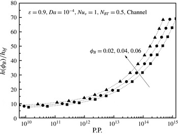
Figure 11. Effects of
 ${\it\phi}_{B}$
on the heat transfer coefficient ratio in a channel filled with a nanofluid-saturated metal foam.
${\it\phi}_{B}$
on the heat transfer coefficient ratio in a channel filled with a nanofluid-saturated metal foam.
The effects of
 $N_{BT}$
on the heat transfer ratio
$N_{BT}$
on the heat transfer ratio
 $h({\it\phi}_{B})/h_{bf}$
are illustrated in figure 12. As expected from figure 10, showing the temperature profiles, which are fairly insensitive to
$h({\it\phi}_{B})/h_{bf}$
are illustrated in figure 12. As expected from figure 10, showing the temperature profiles, which are fairly insensitive to
 $N_{BT}$
, the heat transfer ratios obtained with different values of
$N_{BT}$
, the heat transfer ratios obtained with different values of
 $N_{BT}$
almost overlap one another. Figure 13, on the other hand, shows the effects of
$N_{BT}$
almost overlap one another. Figure 13, on the other hand, shows the effects of
 $\mathit{Nu}_{v}$
on the heat transfer coefficient ratio
$\mathit{Nu}_{v}$
on the heat transfer coefficient ratio
 $h({\it\phi}_{B})/h_{bf}$
, which clearly indicates that higher interstitial heat transfer coefficient yields higher macroscopic heat transfer coefficient. Thus, the combination of metal foams and nanofluids results in unconventionally high heat transfer coefficients.
$h({\it\phi}_{B})/h_{bf}$
, which clearly indicates that higher interstitial heat transfer coefficient yields higher macroscopic heat transfer coefficient. Thus, the combination of metal foams and nanofluids results in unconventionally high heat transfer coefficients.

Figure 12. Effects of
 $N_{BT}$
on the heat transfer coefficient ratio in a channel filled with a nanofluid-saturated metal foam.
$N_{BT}$
on the heat transfer coefficient ratio in a channel filled with a nanofluid-saturated metal foam.

Figure 13. Effects of
 $\mathit{Nu}_{v}$
on the heat transfer coefficient ratio in a channel filled with a nanofluid-saturated metal foam.
$\mathit{Nu}_{v}$
on the heat transfer coefficient ratio in a channel filled with a nanofluid-saturated metal foam.
9. Conclusions
The set of macroscopic governing equations appropriate for convective heat transfer in a nanofluid-saturated metal foam were derived rigorously by applying a volume-averaging theory to the microscopic set of modified Buongiorno equations. Unknown terms are mathematically modelled so as to close the set of governing equations. Mechanical dispersion terms, namely, the thermal dispersion term and particle mechanical dispersion term, were considered analytically using a pore-scale conduit model. Thus, dispersion coefficients for both thermal dispersion and particle mechanical dispersion were estimated, using pore-scale profiles for velocity and temperature. It has been found that the present analytical expression for the transverse thermal dispersion based on the pore-scale analysis closely follows the empirical correlation of Calmidi & Mahajan (Reference Calmidi and Mahajan2000). The longitudinal particle mechanical dispersion works either to suppress or to enhance the effective diffusion depending on the sign of the local phase temperature difference, while the transverse counterpart is insignificant and therefore can be neglected. Moreover, a comparison under equal pumping power revealed that a high level of the heat transfer rate (about 80 times more than the case of base fluid convection without a metal foam) may be achieved by a combination of metal foam and nanofluid.
List of symbols
-
$A$
-
Surface area
$(\text{m}^{2})$
-
$a_{f}$
-
Specific surface (
$\text{m}^{-1}$
) -
$A_{int}$
-
Interfacial area between the fluid and solid
$(\text{m}^{2})$
-
$c$
-
Specific heat of nanofluid (
$\text{J}~\text{kg}^{-1}~\text{K}^{-1}$
) -
$c_{p}$
-
Specific heat of nanoparticle (
$\text{J}~\text{kg}^{-1}~\text{K}^{-1}$
) -
$c_{s}$
-
Specific heat of solid phase (
$\text{J}~\text{kg}^{-1}~\text{K}^{-1}$
) -
$Da$
-
Darcy number
-
$D_{B}$
-
Brownian diffusion coefficient
$(\text{m}^{2}~\text{s}^{-1})$
-
$D_{T}$
-
Thermophoretic diffusion coefficient
$(\text{m}^{2}~\text{s}^{-1})$
-
$d_{m}$
-
Mean pore diameter (m)
-
$d_{p}$
-
Nanoparticle diameter (m)
-
$f,F,g,G$
-
Profile functions
-
$Hg$
-
Hagen number
-
$h$
-
Wall heat transfer coefficient (
$\text{W}~\text{m}^{-2}~\text{K}^{-1}$
) -
$h_{v}$
-
Volumetric heat transfer coefficient (
$\text{W}~\text{m}^{-3}~\text{K}^{-1}$
) -
$H$
-
Channel height (m)
-
$k$
-
Thermal conductivity of nanofluid (
$\text{W}~\text{m}^{-1}~\text{K}^{-1}$
) -
$k_{BO}$
-
Boltzmann constant (
$\text{J}~\text{K}^{-1}$
) -
$k_{dis}$
-
Dispersion thermal conductivity (
$\text{W}~\text{m}^{-1}~\text{K}^{-1}$
) -
$k_{stag}$
-
Stagnant thermal conductivity (
$\text{W}~\text{m}^{-1}~\text{K}^{-1}$
) -
$K$
-
Permeability
$(\text{m}^{2})$
-
$\mathit{Nu}_{v}$
-
Interstitial Nusselt number
-
$Le$
-
Lewis number
-
$n_{j}$
-
Unit vector pointing outwards from fluid side to solid side
-
$n_{BT}$
-
Microscopic Brownian and thermophoretic diffusivity ratio
-
$N_{BT}$
-
Macroscopic Brownian and thermophoretic diffusivity ratio
-
$\mathit{Nu}_{H,R}$
-
Nusselt number
-
$\mathit{Nu}_{v}$
-
Interstitial Nusselt number
-
$p$
-
Pressure (Pa)
-
$Pe$
-
Péclet number
-
$Pr$
-
Prandtl number of nanofluid
-
$\text{P.P.}$
-
Dimensionless pumping power
-
$q_{0}$
-
Wall heat flux (
$\text{W}~\text{m}^{-2}$
) -
$r$
-
Radial coordinate (m)
-
$R$
-
Tube radius (m)
-
$t$
-
Time (s)
-
$T$
-
Absolute temperature (K)
-
$u_{i}$
-
Velocity vector (
$\text{m}~\text{s}^{-1}$
) -
$V$
-
Representative elementary volume
$(\text{m}^{3})$
-
$x_{i}$
-
Cartesian coordinates (m)
-
$x,y,z$
-
Cartesian coordinates (m)
-
${\it\gamma}$
-
Parameter associated with temperature ratio
-
${\it\varepsilon}$
-
Porosity
-
${\it\varepsilon}^{\ast }$
-
Effective porosity
-
${\it\varsigma}_{k}$
-
Transverse thermal dispersion coefficient
-
${\it\eta}~({\it\zeta}=1-{\it\eta})$
-
Dimensionless radial coordinate
-
${\it\mu}$
-
Viscosity (Pa s)
-
${\it\nu}$
-
Kinematic viscosity of nanofluid
$(\text{m}^{2}~\text{s}^{-1})$
-
${\it\rho}$
-
Density of nanofluid
$(\text{kg}~\text{m}^{-2})$
-
${\it\phi}$
-
Nanoparticle volume fraction


Special symbols
-
$\tilde{{\it\varphi}}$
-
Deviation from intrinsic average
-
$\bar{{\it\varphi}}$
-
Average over the cross-section
-
${\it\varphi}^{\ast }$
-
Dimensionless variable
-
$\langle {\it\varphi}\rangle$
-
Darcian average
-
$\langle {\it\varphi}\rangle ^{f,s}$
-
Intrinsic average


Subscripts and superscripts
-
$B$
-
Bulk mean
-
$bf$
-
Base fluid
-
$dis$
-
Dispersion
-
$f$
-
Fluid phase
-
$p$
-
Nanoparticle
-
$s$
-
Solid phase
-
$w$
-
Wall


