


INTRODUCTION
Zoonotic visceral leishmaniasis (ZVL) is endemic in Mediterranean Europe, where the causative agent Leishmania infantum is transmitted by phlebotomine sandflies of the subgenus Phlebotomus (Larroussius) (Ready, Reference Ready2010), but its surveillance and control are neglected compared with research efforts (Dujardin et al. Reference Dujardin, Campino, Cañavate, Dedet, Gradoni, Soteriadou, Mazeris, Ozbel and Boelaert2008). There are estimated to be only 700 new human cases of ZVL per year in southern Europe (Dujardin et al. Reference Dujardin, Campino, Cañavate, Dedet, Gradoni, Soteriadou, Mazeris, Ozbel and Boelaert2008), and some people develop cutaneous lesions. However, the seroprevalence in the domestic dog, the only proven reservoir host (Quinnell and Courtenay, Reference Quinnell and Courtenay2009), is often 20% (Dujardin et al. Reference Dujardin, Campino, Cañavate, Dedet, Gradoni, Soteriadou, Mazeris, Ozbel and Boelaert2008), sufficiently high to pose a serious risk of re-emergence of human disease, especially in immuno-suppressed people (Ready, Reference Ready2010). Human cases are not usually infectious to sandfly vectors, but the parasite has been exported from Europe in the canine reservoir hosts, historically to Latin America where it now causes much fatal infantile disease (Romero and Boelaert, Reference Romero and Boelaert2010) and recently even to North America in fox hounds (Duprey et al. Reference Duprey, Steurer, Rooney, Kirchhoff, Jackson, Rowton and Schantz2006).
The control of canine leishmaniasis (CanL) is considered to be the best way of reducing the incidence of human disease in ZVL foci (Quinnell and Courtenay, Reference Quinnell and Courtenay2009) and one way of controlling any spread northwards in Europe (Ready, Reference Ready2010). Targeted control would be assisted by predictive risk maps of CanL, but unfortunately these do not exist, even in Europe where there have been numerous surveys and incidence has been mapped for positive point locations or administrative areas (Trotz-Williams and Trees, Reference Trotz-Williams and Trees2003). The current report investigates the challenges of producing a predictive risk map of CanL for western Europe, based on the authors' databasing of historical records of CanL during the EU EDEN project (Emerging Diseases in a changing European eNvironment; http://www.eden-fp6project.net). Records for Eastern Europe were included in our database, but they are not analysed in the current report because they are relatively few in number and the transmission cycles are biogeographically distinct (Ready, Reference Ready2010). Only 2 sandflies, Phlebotomus perniciosus and P. ariasi, have been incriminated as vectors in Portugal, Spain and France, and the former is also the most widespread vector in Italy, where P. perfiliewi and P. neglectus pose regional threats. Further east, the vectors are P. perfiliewi, P. neglectus and P. tobbi.
Of all the CanL records we found in the literature and personal files, only those from random surveys of dog populations were targeted for our risk mapping, in order to lessen the chances of analysing populations of mixed geographical origins, including travel cases, or biasing prevalence estimates by missing asymptomatic seropositive dogs. Multivariate logistic regression models were built, using a GIS framework, to find the main predictors of CanL prevalence in western Europe or France alone based on a range of variables, including remotely-sensed climatological and vegetation indices.
MATERIALS AND METHODS
Developing a European database of CanL
The EDEN subproject on leishmaniasis developed a database of all surveys of CanL carried out in Europe and other Mediterranean countries from 1965. A standardized Microsoft® Office Excel worksheet included information related to: publication or dataset; survey type, date, location and environment; method of selecting dogs to be screened; method(s) of diagnosis of infection; dog travel history, breed, age and lifestyle; number of dogs tested and number positive.
For the present study, the data-gathering teams in Portugal (1), Spain (3), France (1) and Italy (1) performed a systematic search for published and unpublished reports in their regions, based on their expert knowledge of data sources. Data entries were standardized by the analytical team in the UK, based on clarifications provided by the data gatherers. The present analysis included only surveys that provided estimates of CanL prevalence based on serological diagnosis. Surveys were excluded from the analysis if 1 or more of the following criteria applied: CanL prevalence could not be estimated either directly or indirectly; the method of diagnosis was not serological (but was based solely on clinical signs, microscopy or molecular characterization); dogs were clearly not sampled ‘randomly’ from a settlement or administrative unit (excluded were positive cases reported by veterinary clinics or other cases possibly associated with passive detection and unknown combinations of localities); data were duplicated and reported more completely in another publication; location was missing or unable to be geo-positioned; and, environmental data were lacking.
Only a minority of reports included geographical coordinates. Most records mentioned the nearest settlement, which was geo-positioned using Google Earth (http://earth.google.com; accessed 2 February 2009). The survey date was potentially an explanatory variable, and so it was derived by (a) averaging the survey's start and end years, or (b) using one of those two dates if the other was missing, or (c) using the year of publication if survey dates were not reported.
Environmental data
Data for long-term climatic averages (based on the period 1961–1990) of monthly precipitation, relative humidity, mean temperature and mean diurnal temperature range were obtained at a spatial resolution of 10 arc-minutes from the Climatic Research Unit, University of East Anglia, UK (New et al. Reference New, Lister, Hulme and Makin2002). Monthly data were aggregated into averages for the warm months (May to September) and for the cold months (October to April). Remotely sensed (MODIS v4), Fourier-processed data (Rogers et al. Reference Rogers, Hay and Packer1996) for day-time (LSTD) and night-time (LSTN) land surface temperature, middle infrared reflectance (MIR) and Enhanced vegetation index (EVI) for the period 2001–2005 were produced by Professor David Rogers and his team (Spatial Ecology and Epidemiology Research Group, Department of Zoology, Oxford University) and obtained from the EDEN project data archive (http://ergodd.zoo.ox.ac.uk/EDEN/index.php?p=1; accessed 2 March 2009). These data have a spatial resolution of 1 km (250 m for EVI) and include separate products relating to the means, amplitudes and phases of annual, biannual and tri-annual cycles. Elevation data were derived from the GLOBE digital elevation model (spatial resolution 1 km) (US National Geophysical Data Center (NGDC), National Oceanic & Atmospheric Administration (NOAA) Satellite and Information Service. Available: http://www.ngdc.noaa.gov/; accessed 2 March 2009).
Statistical model building
CanL seroprevalence was modelled as a binomial variate: the number of dogs examined and dogs found exposed to Leishmania infection at each survey location. To overcome the dependency of observations at the same location, the association between risk of exposure to infection and the environmental covariates was determined using fixed-effects grouped logistic regression with robust standard errors (Rogers, Reference Rogers1993; Rabe-Hesketh and Everitt, Reference Rabe-Hesketh and Everitt2004) in the statistical package Stata (version 10; StataCorp, College Station, Texas, USA). Binary logistic regression (logit command in Stata) is more frequently used for statistical modelling, but this would have required splitting CanL seroprevalence into 2 categories and, thereby, losing information (Rabe-Hesketh and Everitt, Reference Rabe-Hesketh and Everitt2004). In addition, global spatial structures within the seroprevalence data and among model Pearson residuals from multivariate regression analysis were evaluated using semivariograms estimated using the R module GeoR (Ribeiro and Diggle, Reference Ribeiro and Diggle2001). Semivariograms show the spatial dependence of the variable of interest as a scatter plot, and as such provide a means of assessing visually the presence of spatial autocorrelation (Pullan et al. Reference Pullan, Bethony, Geiger, Cundill, Correa-Oliveira, Quinnell and Brooker2008).
Prior to multivariate analysis, univariate binomial logistic regression analyses were carried out to test for associations between seroprevalence and each of the 46 environmental variables, as well as the potentially confounding variable of the survey country. Predictors that were significant at the 10% probability level were retained. The uncentred variance inflation factor (VIF) was used to screen for co-linearity between the retained environmental continuous variables (Rabe-Hesketh and Everitt, Reference Rabe-Hesketh and Everitt2004). Within a group of themed environmental variables, those with VIF ⩾10 were excluded one by one. The procedure was repeated to test for co-linearity between the variables of different groups. The remaining variables were included in a multivariate binomial logistic regression model, for which a backward stepwise selection procedure was performed, excluding the variables with the highest Wald test P-value until all the variables in the model had P<0 05.
Some of the variables retained in the model were non-linear, and these were transformed if this improved the model fit. We found the best transformation for each predictor, starting with the one with the smallest P-value in the linear model, and then transforming the predictor with the next smallest P-value. The non-linearity of each variable (x) was explored by a quadratic polynomial transformation and by 7 fractional polynomial transformations of the first degree (FPs), namely 1/x2, 1/x, 1/x0 5, ln(x), x0 5, x2, and x3 (Royston et al. Reference Royston, Ambler and Sauerbrei1999; Hosmer and Lemshow, Reference Hosmer and Lemshow2000). The best-fit transformation is the one that produces the largest reduction in the residual deviance. The quadratic polynomial transformation was selected if it decreased deviance by more than 5 99 compared with the best fit FP. Otherwise, the best fit FP was selected if it decreased deviance by more than 3 84 compared with the linear (i.e. untransformed) variable. If the decrease in deviance was less, then the variable remained linear. This process was repeated several times until no further FP transformations were indicated for the multivariate model without clustering, and then the same transformation was applied when fitting the final model with clustering (Hosmer and Lemshow, Reference Hosmer and Lemshow2000).
The same method was used to build 2 additional models. For the four-country dataset, a separate model included diagnostic method and survey year, to assess whether they improved the accuracy of the model predictions. A separate model was also built for the data from France alone, in order to investigate better any effect of country on accuracy.
Model validation
The predictive performance of each model was assessed by using a 10-fold cross-validation approach (Hastie et al. Reference Hastie, Tibshirani and Friedman2001; Tibshirani et al. Reference Tibshirani, Hastie, Narasimhan and Chu2002). Briefly, the CanL seroprevalence dataset was split randomly into 10 approximately equal-sized parts. The final multivariate logistic model was fitted on 90% of the data points, and then used to predict the seroprevalence of the remaining 10% (the validation set). This procedure was performed 10 times, each time with 1 of the 10 dataset parts acting as the validation set. The seroprevalences predicted by all the validation sets were then compared with the observed values for the same locations. For each of the validation sets the predictive performance of the model was tested by determining the capacity of the model to predict either point-values of seroprevalence – using the correlation coefficient as a measure of linear association between the predicted and the observed values (Gething et al. Reference Gething, Noor, Gikandi, Hay, Nixon, Snow and Atkinson2008; Hay et al. Reference Hay, Guerra, Gething, Patil, Tatem, Noor, Kabaria, Manh, Elvazar, Brooker, Smith, Moyeed and Snow2009) – or the correct endemicity class. Three endemicity classes were considered: low (<5% seroprevalence), medium (5–20%), and high risk (>20%). The capacity of the model to predict the correct endemicity class was assessed using the area-under-curve (AUC) of a receiver-operating-characteristic (ROC) curve, which plots sensitivity versus one minus specificity for each endemicity class (Brooker et al. Reference Brooker, Hay and Bundy2002; Hay et al. Reference Hay, Guerra, Gething, Patil, Tatem, Noor, Kabaria, Manh, Elvazar, Brooker, Smith, Moyeed and Snow2009). AUC values indicate the agreement between the observed and predicted endemicity class: poor, 0 51–0 70; reasonable, 0 71–0 90; and excellent, >0 9 (Brooker et al. Reference Brooker, Hay and Bundy2002; Hay et al. Reference Hay, Guerra, Gething, Patil, Tatem, Noor, Kabaria, Manh, Elvazar, Brooker, Smith, Moyeed and Snow2009). The prediction accuracy was further assessed by a contingency table and by calculating the percentage of points classified in the correct endemicity class or in a non-adjacent class (Hay et al. Reference Hay, Guerra, Gething, Patil, Tatem, Noor, Kabaria, Manh, Elvazar, Brooker, Smith, Moyeed and Snow2009). The validation statistics for all 10 dataset parts were averaged to compute the overall accuracy of the predictions.
Producing a risk map of CanL seroprevalence
Each statistical model was then used to estimate CanL seroprevalence for a country, based on the predictor values available from remotely sensed images for a 1 km-square grid. Finally, the predicted CanL risk was converted into 1 of 5 endemicity classes: low (<5% seroprevalence), medium-low (5–10%), medium-high (10 01–20%), high (20 01–30%) and very high risk (>30%), and the predicted seroprevalence was mapped using ArcGIS v. 9.2 (ESRI, Redlands, CA, USA). Seroprevalence was mapped only for the pixels where the environmental values were within the range of those in the survey locations.
RESULTS
Database of CanL in Europe
The historical CanL database included cross-sectional surveys, prospective surveys, laboratory records, cases reported at veterinary clinics and case reports. It contained 2187 surveys, including 33 from Croatia, 26 from Greece and 55 from Turkey. There was a total of 2073 reports from Portugal, Spain, France and Italy, of which 947 (45 7%) were included and 1126 were excluded from the current analysis based on the criteria reported above. The most frequent exclusion reasons were non-random sampling (n=849; 75 4%), missing data for the number of dogs tested or positive (n=595; 52 8%) and non-serological diagnosis (n=258; 22 9%). Of the latter, 117 were solely based on microscopy, 58 on culture, 47 on molecular characterization, and 36 on clinical signs. The datasets with the included and excluded CanL seroprevalence surveys can be obtained from the corresponding author.
The remaining 947 surveys were analysed, and the reports included 124 publications. The surveys were undertaken between 1971 and 2006 inclusive (75% after 1985, and 50% after 1992) and involved 504 369 dogs tested for exposure to Leishmania infections. The data analysed are summarized in Table 1 and mapped in Fig. 1. Of the analysed surveys, most were conducted in Italy (377; 40%), followed by Spain (213; 22%), Portugal (188; 20%) and France (169; 18%). The median number of dogs tested per survey was 67, being highest in Italy (168) and lowest in Spain (39). The frequency distribution of the number of dogs per survey was highly right skewed, with the maxima being 30 001 for Italy, 7067 for France, 1803 for Spain and 1024 for Portugal. Surveys were conducted between latitudes 35 5° and 47 5° North and longitudes 9 3° West and 17 6° East. The analysed records covered altitudes of 1–1838 m above sea level (median 204 m a.s.l.). Most surveys (99%) were conducted below 1000 m a.s.l. (3 at 1000–1500 m a.s.l. in France; and 6 at 1000–1500 m a.s.l. and 1 at 1838 m a.s.l. in Spain). The diagnostic method most commonly used was the indirect fluorescent antibody test (IFAT), both overall (77%) and in each country, and the most frequent IFAT cut-off was equal to or above the current minimum standard of 1:80. The proportion of surveys using an IFAT cut-off <1:80 was 35 4% in Italy, 19 2% in Portugal, 2 4% in Spain and 0% in France. The other serological diagnostic methods most frequently used were ELISA, DOT-ELISA and the direct antibody test (DAT).
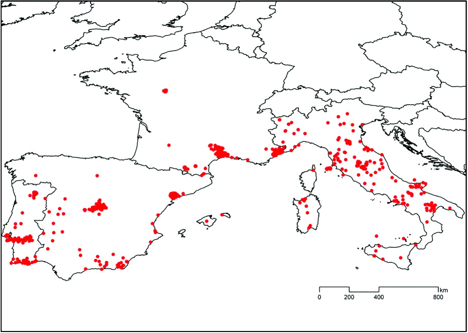
Fig. 1. Distribution of all 947 serological surveys of canine leishmaniasis included in the analyses and modelling of its seroprevalence.
Table 1. Seroprevalences of canine leishmaniasis and number of dogs tested for all surveys analysed

a Percentage of surveys out of the total of surveys in all countries. Percentages for categories total 100%, except for altitude because this was not found for 11 surveys (5 in France, 4 in Italy and 2 in Portugal).
b Including CIE, IFAT and CIE, LST. [IFAT: Indirect Fluorescence Antibody Test. ELISA: Enzyme-Linked Immunosorbent Assay. DAT: Direct Agglutination Test. CIE: Counter-immunoelectrophoresis. LST: Leishmanin Skin Test].
c Percentage of dogs tested calculated out of the total of dogs tested in all countries.
The overall CanL seroprevalence was 23 2% (116,968/504,369), and 5% of the surveys recorded seroprevalences >40%. Point seroprevalences >80% were recorded in Italy, Portugal and Spain, but the maximum in France was only 43%. The median seroprevalence was 10%, being highest in Italy (17 7%), followed by France (8%), Portugal (7 3%) and Spain (5 9%). Zero seroprevalences were recorded in 14 7% of the surveys, being more frequent in Spain (25%), followed by Portugal (20%), France (14%), and Italy (6%).
Statistical models
Four-country model
Among the 49 variables screened by univariate analysis (Table 2), 32 were significantly associated with CanL seroprevalence at the 10% probability level: diagnostic method, survey year, country, altitude, latitude, 21 Fourier-transformed remotely sensed (RS) variables from 4 environmental groups, and 6 variables from 4 climatic groups. Of the latter 27 variables, 19 were excluded due to co-linearity, leaving 11 variables to be tested for inclusion in the multivariate model. These consisted of country, altitude, latitude and 8 Fourier-transformed RS variables relating to night-time land surface temperature (minimum (LSTNmn), amplitude of the tri-annual cycle (LSTNa3)), day-time land surface temperature (amplitude of the bi-annual cycle (LSTDa2), phase of the tri-annual cycle (LSTDp3)), and enhanced vegetation index (minimum (EVImn), amplitude of the annual cycle (EVIa1), and phases of the annual and tri-annual cycles (EVIp1, EVIp3)). Of these, 7 variables remained in the final multivariate model (Table 3). The association with seroprevalence was inversely U-shaped for some predictors (i.e. the highest seroprevalence was observed at intermediate values), namely altitude, LSTNmn, LSTNa3 and to a much lesser degree EVIp1, and so all were used with a quadratic transformation. When testing for the confounding effect of diagnostic method and survey year, only the latter dropped from the multivariate model. However, diagnostic method was not retained, because it did not substantially improve the accuracy of the model predictions. Semivariograms were estimated on the basis of both observed prevalence and Pearson residuals from multivariate models, to investigate the removal of spatial trends potentially related to environmental variables. Both analyses produced unbounded semivariograms (not shown) in which semivariance increased steadily with increasing distance (spatial lags) between observations. In the absence of any clear spatial structure in the prevalence data, modelling was restricted to a non-spatial regression analysis. The final model equation was: CanL seroprevalence=(exp(p)/(1+exp(p))×100; where p=−2 67413−0 5203425×country_2−1 486901×country_3−1 627514×country_4+0 0015933×altitude−8 76×10−7×(altitude)2+0 1632941×LSTNmn−0 0167179×(LSTNmn)2+4 346963×LSTNa3−2 562916×(LSTNa3)2+0 0874507×1/√EVIa1+0 136483×EVIp1−0 0361457×(EVIp1)2−0 1942139×(1/EVIp3); and where country_2, country_3 and country_4 were dummy variables for Italy, Portugal and Spain, respectively.
Table 2. Univariate binomial logistic regression analyses to test associations between seroprevalence of canine leishmaniasis in the four countries and each potential explanatory variable

a The last 2 characters denote the output from Fourier processing:−a0: mean, mn: minimum, mx: maximum, a1: ampli-tude of annual cycle, a2: amplitude of bi-annual cycle, a3: amplitude of tri-annual cycle, p1: phase of annual cycle, p2: phase of bi-annual cycle, p3: phase of tri-annual cycle;
b DTR: diurnal temperature range, TMP: mean temperature, PRE: rainfall, REH: relative humidity, summer: May-September, winter: October-April;
* P <0 1 in the univariate analysis.
Table 3. Multivariate binomial logistic regression analysis of the associations between seroprevalence of canine leishmaniasis and each explanatory variable (or risk factor) for the four-country model

a The last 2 characters denote the output from Fourier processing:−mn: minimum, a1: amplitude of annual cycle, a3: amplitude of tri-annual cycle, p1: phase of annual cycle, p3: phase of tri-annual cycle.
b Odds Ratio (OR) was calculated for the reference point of the categories of each variable Xi from the final model: Log Odds=−2 67413 + β iXi. Where β iXi is: for country, −0 5203425×country_2−1 486901×country_3−1 627514×country_4 (where the baseline country is France, and country_2, country_3 and country_4 are dummy variables for country=Italy, Portugal or Spain, respectively); for altitude: 0 0015933×altitude−8 76×10−7×(altitude)2; for LSTNmn: 0 1632941×LSTNmn−0 0167179×(LSTNmn)2; for LSTNa3: 4 346963×LSTNa3−2 562916×(LSTNa3)2; for EVIa1: 0 0874507×1/ √EVIa1; for EVIp1: 0 136483×EVIp1−0 0361457×(EVIp1)2; and for EVIp3: −0 1942139×(1/EVIp3).
c The 95% confidence interval (CI) was calculated according to Pullan et al. (Reference Pullan, Bethony, Geiger, Cundill, Correa-Oliveira, Quinnell and Brooker2008).
France-only model
Following the same method, the only variables remaining in the final multivariate model were altitude, LSTNmn, amplitude of the bi-annual cycle of the night-time land surface temperature (LSTNa2), LSTNa3, amplitude of the annual cycle of middle infrared reflectance (MIRa1) and amplitude of the tri-annual cycle of middle infrared reflectance (MIRa3) (Table 4). The final model equation was: CanL seroprevalence=(exp(p)/(1+exp(p))×100; where p=−5 849738+0 0526301×√altitude +32 16849×MIRa1−129 4284×MIRa3+1 429675×1/√LSTNa2+1 130128×LSTNa3+0 2185278×LSTNmn.
Table 4. Multivariate binomial logistic regression analysis of the associations between seroprevalence of canine leishmaniasis and each explanatory variable (or risk factor) for the France-only model

a The last 2 characters denote the output from Fourier processing:−mn: minimum, a1: amplitude of annual cycle, a2: amplitude of bi-annual cycle, a3: amplitude of tri-annual cycle.
b Odds Ratio (OR) was calculated for the reference point of the categories of each variable Xi from the final model: Log Odds=−5 849738 + βiXi. Where βiX is, for altitude: 0 0526301×√altitude; for LSTNmn: 0 2185278×LSTNmn; for LSTNa3: 1 130128×LSTNa3; for LSTNa2: 1 429675×1/√LSTNa2; for MIRa1: 32 16849×MIRa1; and for MIRa3: −129 4284×MIRa3.
c The 95% confidence interval (CI) was calculated according to Pullan et al. (Reference Pullan, Bethony, Geiger, Cundill, Correa-Oliveira, Quinnell and Brooker2008).
Validation of four-country model
This was performed with 931 surveys, because at least 1 of the environmental variables in the model was missing for 16 records (5 in France, 8 in Italy and 3 in Portugal).
Predicting point-values of CanL seroprevalence: The global correlation coefficient (r) between the predicted and observed seroprevalences was 0 341, and the weakness of this linear agreement was clear in a scatter plot. Predicted seroprevalences were concentrated at ⩽40%, while observed seroprevalences ranged from 0 to 100%. The overall fit did not improve significantly (r=0 352) if only the observed seroprevalences ⩽40% (95% of records) were considered. The country level correlation was considerably stronger for Italy (r=0 432), which had about twice as many surveys as the other 3 countries (r=0 233–0 262).
Predicting endemicity classes of CanL seroprevalence: When comparing the model predictions with the observed seroprevalences in the 931 surveys, 41% of the records were correctly classified to 1 of the 3 endemicity classes (Italy: 48%; Spain: 40%; Portugal: 37%; France: 32%). Only 5 5% were misclassified to a non-adjacent class (Italy: 3 8%; Spain: 4 2%; Portugal: 2 2%; France: 14 6%). Overall AUC statistics for the two extreme seroprevalence classes (<5%, >20%) exceeded the 0 7 threshold for fair to good discrimination (AUC=0 71 and 0 73, respectively), but the AUC for the intermediate class (5–20%) was below the threshold (AUC=0 55). When looking at the results by country, similar results applied to France and Italy, where the model performed best, while in Portugal and Spain the AUC for all CanL seroprevalence classes was below 0 6.
Validation of France-only model
This was performed with 164 of the 169 surveys carried out from 1971 to 2006, because at least 1 of the environmental variables in the model was missing for 5 records.
Predicting point-values of CanL seroprevalence: The global correlation coefficient (r) between the predicted and observed seroprevalences was 0 648. The range of predicted seroprevalences was 2–38%, which is comparable to the observed range of 0–43%.
Predicting endemicity classes of CanL seroprevalence: When comparing the model predictions with the observed seroprevalences in the 164 surveys, 54% of the records were correctly classified to 1 of the 3 endemicity classes, substantially more than those correctly classified for France (32%) by the four-country model. Only 3% were misclassified to a non-adjacent class, substantially fewer than those misclassified for France (14 6%) by the four-country model. Overall AUC statistics for the two extreme seroprevalence classes (<5%, >20%) exceeded the 0 7 threshold for fair to good discrimination (AUC=0 77 and 0 81, respectively), but the AUC for the intermediate class (5–20%) was below the threshold (AUC=0 64).
Risk maps
The predicted CanL seroprevalence was mapped for the four-country model (Fig. 2) and for the France-only model (Fig. 3) using 5 endemicity classes. Pixels were unclassified if their environmental values were outside the range of those in the survey locations. When estimating seroprevalence for the risk maps, a minimum increment was added to each value of EVIp3, EVIa1 and LSTNa2, in order to eliminate any zero values. In the four-country model, EVIp3 and EVIa1 were replaced by EVIp3+0 01 and EVIa1+0 001, respectively; and, in the France-only model, LSTNa2 was replaced by LSTNa2+0 02.

Fig. 2. Risk map for canine leishmaniasis (CanL) in Portugal, Spain, France and Italy based on the four-country model. Predicted CanL seroprevalence was mapped only for the pixels where the predictive environmental values were within the range of those in the survey locations. Other pixels, those outside this mask, are shaded in grey.

Fig. 3. Risk map for canine leishmaniasis (CanL) in France based on the France-only model. Predicted CanL seroprevalence was mapped only for the pixels where the predictive environmental values were within the range of those in the survey locations. Other pixels, those outside this mask, are shaded in grey. The areas marked by red diagonals show France outside the latitudinal range of all the surveys analysed. Latitude was not a predictive variable.
Unclassified pixels were relatively few in number for the four-country model, but considerably higher for the France-only model. For the four-country map, a total of 4034 (6 31%) pixels were unclassified (Italy: 1969 (14 88%); Spain: 661 (3 12%); Portugal: 55 (1 47%)), with 1711 of these pixels being outside the altitude range of the survey locations in the four countries (254 <1 m a.s.l.; 1457 >1838 m a.s.l.), and 50% of the unclassified pixels were located <1492 m a.s.l. For France mapped using the four-country model, a total of 1349 (5 24%) pixels were unclassified, with 575 of these pixels being outside the altitude range of the survey locations in the four countries (81<1 m a.s.l.; 494 >1838 m a.s.l.), and 50% of the unclassified pixels were located <1457 m a.s.l. In contrast, for France investigated by the France-only model, a total of 7998 (31 05%) pixels were unclassified, with 1333 of these pixels being outside the altitude range of the survey locations in France (81<1 m a.s.l.; 1252 >1193 m a.s.l.), and 50% of the unclassified pixels were located <257 m a.s.l. For France, overall, there were almost 13 times more pixels not classified at altitudes ⩽1193 m a.s.l. in the France-only risk map compared with the four-country one.
DISCUSSION
Our database is unique. It is the first time that detailed historical records of CanL in endemic European countries have been collated in this standardized way for such a long period (1965–2006), and the database is an important resource for future eco-epidemiological analyses at country and regional levels. However, like all such databases, its entries mirror the different histories of European teams working with changing diagnostic techniques and public health priorities (Dujardin et al. Reference Dujardin, Campino, Cañavate, Dedet, Gradoni, Soteriadou, Mazeris, Ozbel and Boelaert2008), including the period (1990–1998) when epidemiological investigations of ZVL focused on co-infections with HIV. Partly for these reasons, many records were not suitable for our specific analyses, and we hope this finding will prompt better standardization of prospective surveys when cost effective.
Our use of this database in the current report has produced 2 sets of novel findings. One set arises from the construction of the first explicit risk map for CanL in western Mediterranean Europe and consideration of the lessons to be learned from its apparent deficiencies. The second set of findings relates to the identification of shortcomings in the scope and standardization of CanL surveys, and how these can inform guidelines for future collection of prospective data.
Our best model for western Europe, the four-country model, predicted the seroprevalence of CanL based on 7 variables, namely country, altitude, minimum night-time land surface temperature (LSTNmn), amplitude of the tri-annual cycle of the night-time land surface temperature (LSTNa3), amplitude of the annual cycle of the Enhanced vegetation index (EVIa1), phase of the annual cycle of the Enhanced vegetation index (EVIp1) and phase of the tri-annual cycle of the Enhanced vegetation index (EVIp3). The association with CanL seroprevalence was inversely U-shaped for 4 of the predictors (altitude, LSTNmn, LSTNa3, and to a lesser degree EVIp1), and this can be explained by the ecological requirements of the nocturnal sandfly vectors being met in rural settings on the lower and middle slopes of hills and mountains (often 100–800 m a.s.l.) during the dry Mediterranean summer (Ready, Reference Ready2008; Gálvez et al. Reference Gálvez, Descalzo, Miró, Jiménez, Martín, Dos Santos-Brandao, Guerrero, Cubero and Molina2010a; Mahamdallie et al. Reference Hartemink, Vanwambeke, Heesterbeek, Rogers, Morley, Pesson, Davies, Mahamdallie and Ready2011). The more linear associations with EVIa1 and EVIp3 were negative and positive, respectively, and these findings should be explored by sandfly ecologists. There is no published risk map for CanL in the western Mediterranean to compare with our own. However, our risk map does appear to be inconsistent with the incidence map of Trotz-Williams and Trees (Reference Trotz-Williams and Trees2003), principally by not predicting more high risk areas near the coastal plains of Spain and Portugal, and also by predicting too many high risk areas in southwest, northwest and central France. Chamaillé et al. (Reference Chamaillé, Tran, Meunier, Bourdoiseau, Ready and Dedet2010) used the machine-learning Maxent method to produce an ecological niche model and a risk map for CanL in southern France, and this was based on presence data from our database, including many records from veterinary clinics. Our risk maps differ from theirs by identifying more low-high risk areas in central France and the inland parts of southwest France, as well as by identifying fewer medium-high risk areas in the more coastal parts of southwest France, where the Atlantic influences the climate.
One of the predictors of CanL in our four-country model was country. It is often the case that models differ between nearby countries, and this is true for anthroponotic visceral leishmanisis caused by Leishmania donovani in East Africa (Ready, Reference Ready2008). Model variation between European countries might be explained by geographical differences in climate and seasonality associated with the bioclimatic and ecological requirements of the sandfly species serving as regional vectors. These considerations prompted us to construct a separate model and risk map for France, where both vectors (P. perniciosus and P. ariasi) have overlapping altitudinal ranges throughout much of the Mediterranean region (Ready, Reference Ready2008; Chamaillé et al. Reference Chamaillé, Tran, Meunier, Bourdoiseau, Ready and Dedet2010; Hartemink et al. Reference Hartemink, Vanwambeke, Heesterbeek, Rogers, Morley, Pesson, Davies, Mahamdallie and Ready2011), unlike in Italy where 1 of the 2 main vectors (P. perfiliewi, not P. perniciosus) occurs only in the centre-south of the country (Maroli et al. Reference Maroli, Rossi, Baldelli, Capelli, Ferroglio, Genchi, Gramiccia, Mortarino, Pietrobelli and Gradoni2008). Our best model for France alone, the France-only model, predicted the seroprevalence of CanL based on 6 variables, namely altitude, LSTNmn, amplitude of the bi-annual cycle of the night-time land surface temperature (LSTNa2), LSTNa3, amplitude of the annual cycle of middle infrared reflectance (MIRa1) and amplitude of the tri-annual cycle of middle infrared reflectance (MIRa3). LSTNa2 and MIRa3 were negatively associated with CanL seroprevalence, while the other 4 variables were positively associated with it. The France-only model differs from the four-country model mainly in the replacement of EVI, an index that estimates plant structural variation based on the reflectance of red and near-infrared wavelengths, with MIR, an index that distinguishes better between active vegetation on the one hand and senescent vegetation, soils, rocks or anthropogenic surfaces on the other (Scharlemann et al. Reference Scharlemann, Benz, Hay, Purse, Tatem, Wint and Rogers2008).
The France-only model was found to be better than the four-country model for predicting the seroprevalence of CanL in France, probably because the latter was based mostly on surveys and dogs from Italy (40% and 84%, respectively) rather than France (18% and 7 8%, respectively). The four-country model was a poor global predictor of point values of CanL seroprevalence (correlation coefficient, r=0 341), although the correlation was stronger for survey-rich Italy (r=0 432) than for the other 3 countries (r=0 233–0 262). In comparison, the France-only model gave a much better correlation between the predicted and observed CanL seroprevalences (r=0 648). Based on AUC statistics, both models did provide fair-to-good discrimination (AUC >0 7) for the 2 extreme classes of CanL endemicity (<5%, >20% seroprevalence) but not for the intermediate class (5–20%). Many observed seroprevalences fell within this intermediate class (360 out of 947 overall, and 84 out of 169 in France), which is also true for much of the Mediterranean region (Dujardin et al. Reference Dujardin, Campino, Cañavate, Dedet, Gradoni, Soteriadou, Mazeris, Ozbel and Boelaert2008), and so it is important to consider whether this lack of resolution results from the modelling approach or inadequate sampling.
The statistical methods commonly used to predict the occurrence or distribution of parasitic diseases in relation to environmental variables include discriminant (Rogers and Randolph, Reference Rogers, Randolph, Hay, Graham and Rogers2006) and Bayesian methods (Clements et al. Reference Clements, Moyeed and Brooker2006) as well as logistic regression, both binary (Brooker et al. Reference Brooker, Hay, Issae, Hall, Kihamia, Lwambo, Wint, Rogers and Bundy2001) and binomial (Rabe-Hesketh and Everitt, Reference Rabe-Hesketh and Everitt2004). Binary logistic regression was used successfully for the spatial modelling of anthroponotic visceral leishmaniasis in East Africa (Thomson et al. Reference Thomson, Elnaiem, Ashford and Connor1999). Non-linear discriminant analysis (NLDA) might provide better predictions than logistic regression (Rogers and Randolph, Reference Rogers, Randolph, Hay, Graham and Rogers2006), and it would be interesting to apply it to our datasets. However, we do not believe that NLDA would much improve the resolution of our predictions for those locations where CanL seroprevalence is in the intermediate range of 5–20%. This conclusion stems from the limitations of our climate and RS datasets as well as of the sampling procedures used to obtain our survey data. In common with most spatial models, ours relied on using widely available sets of climate and RS data, which unfortunately cover different time periods and have varying spatial resolutions. None of the resolutions fully captured the variation in the microclimates inhabited by sandflies, which would hinder the inclusion of sandfly density as an explanatory variable in any integrated model (Hartemink et al. Reference Hartemink, Vanwambeke, Heesterbeek, Rogers, Morley, Pesson, Davies, Mahamdallie and Ready2011). We could have modelled CanL seroprevalence over shorter time periods using matching climate surfaces from the EU ENSEMBLES project (http://www.ensembles-eu.org/), in order to improve the risk maps and investigate any effects of climate change. However, this requires the availability of CanL seroprevalence datasets with fewer limitations than those currently available, as now explained.
Our models' poor predictions of CanL seroprevalence in the intermediate range of 5–20% relate to shortcomings in the scope and standardization of CanL surveys. Firstly, there has been a bias towards known rural and peri-urban foci in Mediterranean bioclimate zones, and consequently zero seroprevalence was recorded in only 14 7% of the surveys (14–25% in France, Portugal and Spain, but just 6% in Italy). We recommend that future surveys do not neglect environments at more extreme altitudes (<100 m, >1000 m a.s.l.) and northerly latitudes. Secondly, the most used serological test (IFAT) has not been standardized, e.g. the proportion of surveys using a cut-off of <1/80 was 35 4% in Italy and 19 2% in Portugal, but negligible in Spain (2 4%) and France (0%). The use of low IFAT cut-offs in many surveys in Italy could possibly have produced for this country the highest median seroprevalence (17 7%; 5 9–8% elsewhere) and the lowest frequency of zero seroprevalence (6%; 14–25% elsewhere). We strongly recommend that all published surveys include the proportion of dogs seropositive for each of the serial dilutions of the sera, not just for those making the cut-off, so that records from different periods can be better compared. Improvements in fluorescence microscopy have led to changes in the consensus cut-off, first 1/40 in the 1970s, then 1/80 in the 1990s, and sometimes 1/160 recently. Thirdly, serology only detects a small fraction of resistant dogs and the susceptibles progressing to clinical disease after long incubation (Maia and Campino, Reference Maia and Campino2008). Therefore, ideally, serology should be complemented by molecular screening in horizontal surveys (Lachaud et al. Reference Lachaud, Chabbert, Dubessay, Dereure, Lamothe, Dedet and Bastien2002; Quinnell and Courtenay, Reference Quinnell and Courtenay2009). Lastly, the resolution of the sampling is inadequate, because a point location was very often an assembly point in a large village, to which dogs were brought for screening from a radius of 10 km or more (Rioux and Golvan, Reference Rioux and Golvan1969; Maroli et al. Reference Maroli, Rossi, Baldelli, Capelli, Ferroglio, Genchi, Gramiccia, Mortarino, Pietrobelli and Gradoni2008; Martín-Sánchez et al. Reference Martín-Sánchez, Morales-Yuste, Acedo-Sánchez, Barón, Diaz and Morillas-Marquez2009; Gálvez et al. Reference Gálvez, Miró, Descalzo, Nieto, Dado, Martín, Cubero and Molina2010b). To improve the sampling resolution, we recommend including in the model ‘dog factors’, such as the age and lifestyle of individual dogs recorded as living most of the time in specific geo-referenced habitations. Concerning lifestyle, guard dogs and hunting dogs often have a higher prevalence of CanL than pet dogs that sleep indoors (Lanotte et al. Reference Lanotte, Rioux, Croset and Vollhardt1978; Martín-Sánchez et al. Reference Martín-Sánchez, Morales-Yuste, Acedo-Sánchez, Barón, Diaz and Morillas-Marquez2009; Gálvez et al. Reference Gálvez, Miró, Descalzo, Nieto, Dado, Martín, Cubero and Molina2010b). A potentially important explanatory variable missing from our modelling is dog density. Estimates have been used for ecological niche modelling (Chamaillé et al. Reference Chamaillé, Tran, Meunier, Bourdoiseau, Ready and Dedet2010) and R0 modelling (Hartemink et al. Reference Hartemink, Vanwambeke, Heesterbeek, Rogers, Morley, Pesson, Davies, Mahamdallie and Ready2011) of CanL or its vectors in southern France, but these estimates of dog density were based on human population densities that were low and varied little per km2 in the rural areas characteristic of CanL.
As a result of these shortcomings, our risk maps can not be expected to have much predictive power within many CanL foci. It might not always be cost effective to produce high resolution risk maps within CanL foci, for which it will be necessary to follow all our recommendations, but the consequences of not doing so ought to be assessed when agreeing guidelines for collecting prospective data. In contrast, it should be less challenging to improve spatial models so that different geographical regions can be compared. Then, our relatively straightforward method of producing risk maps would be more useful for predicting any northward emergence of CanL and helping to plan barrier methods of control, based currently on topical insecticides (deltamethrin-impregnated dog collars and pour-ons) not dog culling (Quinnell and Courtenay, Reference Quinnell and Courtenay2009) and hopefully on vaccines (Ready, Reference Ready2010). Already, we have demonstrated that country-level risk maps can distinguish well between areas with high (>20%) and low (<5%) CanL seroprevalences (only 3% misclassified using the France-only model) and that seroprevalences are invariably low in areas of CanL emergence. For example, seroprevalence is usually <5% throughout northern Italy above latitude 45 50 N, where CanL has emerged within the last 20 years (Maroli et al. Reference Maroli, Rossi, Baldelli, Capelli, Ferroglio, Genchi, Gramiccia, Mortarino, Pietrobelli and Gradoni2008). The improvement of spatial models for predicting CanL emergence in Europe depends on carrying out new standardized serological and molecular surveys in central and northern Europe as well as at extreme altitudes (<100 m, >1000 m a.s.l.) in Mediterranean locations with comparable land covers. Without such sampling, predictions will not be possible for many regions of interest, such as much of France above 47 50 N, which is the approximate northern limit of our records and of the risk map produced by ecological niche modelling (Chamaillé et al. Reference Chamaillé, Tran, Meunier, Bourdoiseau, Ready and Dedet2010). The complexities of predicting the effects of climate change (Kovats et al. Reference Kovats, Campbell-Lendrum, McMichael, Woodward and Cox2001) lessen the likelihood of risk maps being used to predict the spread of CanL in response to global warming.
ACKNOWLEDGEMENTS
This work is dedicated to Professor Clive R. Davies, who initiated the research but passed away in March 2009. We thank the other members of the EDEN-Leishmaniasis sub-project who helped to construct the database, namely Maria Antoniou and the team at the University of Heraklion (Greece), Robert Farkas and his team in the Faculty of Veterinary Science of Budapest (Hungary), and Yusuf Ozbel and his team in the University of Ege (Turkey). We are grateful for advice on statistical analyses from Francesco Checchi and Simon Brooker of the London School of Hygiene and Tropical Medicine, London, as well as Archie Clements and Ricardo Magalhães of the School of Population Health, University of Queensland, Australia.
FINANCIAL SUPPORT
This work was funded by a grant (GOCE-2003-010284) of the European Union awarded to the EDEN (Emerging Diseases in a changing European eNvironment) project. The publication is catalogued by the EDEN Steering Committee as EDEN0262 (www.edenfp6project.net). Its contents are the sole responsibility of the authors and do not necessarily reflect the views of the European Commission. The funders had no role in study design, data collection and analysis, decision to publish, or preparation of the manuscript. The authors have declared that no competing interests exist.


