


Introduction
Punctuated equilibrium theory (PET) describes policy regimes as mostly stable with periods of rapid, large changes. The dynamics between incremental and punctuated changes apply, for example, throughout public budgeting. Foundational research in PET has identified this pattern of budgetary change in a variety of settings in local, state and federal budgeting (Jones et al. Reference Jones, Baumgartner and True1998; Jones et al. Reference Jones, Sulkin and Larsen2003; Breunig and Koski Reference Breunig and Koski2006). Scholarship has progressed from simply identifying the anticipated pattern of punctuations to examining the characteristics of public institutions that lead to more punctuated (or more incremental) budgetary processes. Organisational performance, personnel turnover, organisation size, level of centralisation and organisational history are all features that scholars have found to influence the frequency of punctuated budgetary changes in public organisations (Robinson et al. Reference Robinson, Caver, Meier and O’Toole2007; Robinson et al. Reference Robinson, Flink and King2014; Flink Reference Flink2017).
Recent research in PET explores not just the shape of the distribution of all budgetary changes for a time period, but the occurrence of punctuations at specific points in time. The shape of the distribution conceals the temporal pattern of punctuations. Did punctuations occur year after year or were they spread over time? Research has shown that large changes are clustered together – one large budgetary punctuation leads to more budgetary punctuations (Robinson et al. Reference Robinson, Flink and King2014). Missing in this line of research is the direction of the punctuation – positive or negative. Are positive and negative large budgetary changes grouped together? Or, are positive and negative punctuations clustered separately by their direction?
This article explores these questions in over 1,000 local government entities, Texas school districts. Two models of budgetary punctuations are proposed. First is the corrective model in which positive and negative budgetary punctuations are paired. When budgets have a sharp decrease, a major increase is likely to occur in the next year or two. Likewise, a positive budgetary punctuation is followed by a negative punctuation. In this model, funding returns to a roughly equilibrium level; punctuations are corrective in pairs. The other model, the trending model, describes budgetary punctuations as cumulative trends – positive or negative budgetary punctuations are grouped together with similarly directed changes. This pattern of punctuations leads to a new base level of funding (much higher or much lower) for a programme.
In multiple logit models, results consistently support the corrective model of budgetary punctuations. When organisations make a rapid, large budgetary change, they more often follow with a budgetary move in the opposing direction than they repeat large changes in the same direction. Further exploration into how budgetary changes respond from punctuations illustrates that once a budgetary punctuation occurs, there is a general shift of budgetary changes (medium and punctuated) in the opposite direction. In a final analysis, it is found that when positive and negative punctuations occur in consecutive years, they are not fully corrective. On average, punctuation pairs appear to keep a short run equilibrium, but the standard deviations of the distributions are large.
Literature review
The origins of incrementalism and its critics
The study of policy change has taken on many forms and proceeded along many paths over the decades. One approach to the study of this broad question has focussed on the nature of the systems that create policy and how these systems constrain the speed and breadth of policy change.
One strain of this research tradition is of particular interest to the study of budgets. Wildavsky (Wildavsky Reference Wildavsky1964; Wildavsky and Caiden Reference Wildavsky and Caiden1988) drew from the prior tradition on incremental policy change – most often associated with Lindblom (Reference Lindblom1959) – to argue that budgetary processes (and, in particular, the federal budgetary policy process) are incremental. Budgets represent compromises between diverse actors and any proposed large change threatens the existing coalitions. As a result, budgetary changes tend to be small and incremental.
There was an almost immediate reaction to the strong form of Wildavsky’s incrementalist characterisation of the budgetary process. Schulman (Reference Schulman1975) argued that there were important counter-examples to the notion that incrementalism was a covering law for policy change processes. He argued that certain policy domains could not proceed incrementally because they could not be subdivided into smaller parts. His signal example is space policy and NASA. One cannot build slowly towards a space programme, Schulman argued. One has to make large (in an absolute sense) and nonincremental (in a sense of changes from previous years) change to proceed in these domains of policy.
The resulting debate between proponents of incrementalism as a generally applicable covering law and critics who pointed to counter-examples continued for decades. This debate was further complicated by drift and confusion within the meaning of various terms in their debate including how one should define and measure incrementalism (Wanat Reference Wanat1974; Tucker Reference Tucker1982; Berry Reference Berry1990; John and Bevan Reference John and Bevan2012). Scholars used incrementalism as a descriptive, explanatory, normative and a predictive theory. Each of those theoretical lenses has yielded various ways for incrementalism to be measured.
Punctuated equilibrium approaches
Cross-application of a theory from palaeontology overcame the impasse between incrementalism and its critics. Baumgartner and Jones (Reference Baumgartner and Jones2009) argued that policy changed proceeded through two separate patterns. Most of the time, policy change was slow – as the incrementalists had argued. However, conditions could create a period wherein large change (punctuated change) is possible through the operation of positive attention cycles and dramatic external events – consistent with many of the critics of incrementalism. PET bridged the divide between theories of fast and slow policy change by acknowledging both dynamics exist in the policy process.
The resulting theory of punctuated policy change led to specific predictions about the distribution of policy changes. Particularly, scholars expected the distribution to have a leptokurtic shape – a tall centre and heavy tails of the distribution. Some of the earliest tests of the predictions of the punctuated equilibrium model used budgetary changes as the indicator of policy change (Jones et al. Reference Jones, True and Baumgartner1997; Jones et al. Reference Jones, Baumgartner and True1998). These investigations found support for the punctuated equilibrium model of policy change in the observed distribution of budgetary changes in federal budgetary categories.
The study of the distributions of policy-relevant outputs spreads rapidly to accommodate tests in various stages of the United States (US) federal policy-making process (Jones et al. Reference Jones, Sulkin and Larsen2003), US state-level budgetary data (Breunig and Koski Reference Breunig and Koski2006) and US school district-level data (Robinson Reference Robinson2004). Tests also spread to other political system to find similar patterns of policy change in a wide range of nations (Breunig Reference Breunig2006; Baumgartner et al. Reference Baumgartner, Breunig, Green-Pedersen, Jones, Mortensen, Nuyte-mans and Walgrave2009). The result of these various studies was a persuasive case that the mixture of incremental and punctuated policy changes characterized all policy systems studied (Jones et al. Reference Jones, Baumgartner, Breunig, Wlezien, Soroka, Foucault, François, Green-Pedersen, Koski, John, Mortensen, Varone and Walgrave2009). This empirical phenomenon was also characterized as the Dynamic Model of Choice for Public Policy (Jones and Baumgartner Reference Jones and Baumgartner2005; Jensen et al. Reference Jensen, Mortensen and Serritzlew2016).
Hypothesis testing
The distributional approach to punctuated policy change has revealed a great deal about patterns common across institutional environments. However, the approach is limited in the sorts of hypotheses it can test – in part because comparisons across data distributions call for several large databases. A separate methodological tradition emerged that tested hypotheses about how characteristics of the policy systems could lead to different expectations of change. Notably, this approach sought research designs more similar to traditional regression-based hypothesis testing.
Jordan’s (Reference Jordan2003) work on local government expenditures represents an early example of this tradition. Jordan defined a threshold beyond which a change could be categorized as nonincremental (a “punctuation”). She then compared different types of local government expenditures (police, highways, public buildings, etc.) to identify which most closely fit the expectations of PET.
Robinson adopted a similar approach to studying local government expenditures because of the leverage they provide on questions of institutional determinants of policy change. The earliest work adapted the distributional methodology to direct hypothesis testing (Robinson Reference Robinson2004) comparing school districts with high and low values of bureaucratisation. The later work adopted a more direct categorisation of each budgetary outcome as incremental, moderate or large changes (Robinson et al. Reference Robinson, Caver, Meier and O’Toole2007). This hypothesis testing approach allowed for multivariate testing within a regression context and compared the influence of bureaucratisation and organisation size on the propensity of an organisation to experience punctuated budgetary change – while allowing for some control variables as well. The approaches of Jordan and Robinson opened up a methodological space for testing hypotheses for factors related to increased or decreased rates of nonincremental policy change.
Recent innovations
Recent work has further refined and extended the hypothesis testing approach to studying punctuated or nonincremental budgetary change.
Some work has built directly on the distributional analysis methodology to construct comparisons more amenable to formal hypotheses testing – notably through the use of l-kurtosis measures. L-kurtosis provides a normed characterisation of a distribution that facilitates comparison across samples – a necessity for comparison of samples of budgetary change. The resulting methodology has undergirded studies of American state budgets (Breunig and Koski Reference Breunig and Koski2006, Reference Breunig and Koski2012) and cross-national comparisons (Breunig Reference Breunig2006; Baumgartner et al. Reference Baumgartner, Breunig, Green-Pedersen, Jones, Mortensen, Nuyte-mans and Walgrave2009; Jones et al. Reference Jones, Baumgartner, Breunig, Wlezien, Soroka, Foucault, François, Green-Pedersen, Koski, John, Mortensen, Varone and Walgrave2009).
Others have further developed our understanding of the institutional characteristics that facilitate or impede nonincremental budgetary changes. Ryu (Reference Ryu2011a, Reference Ryu2011b, Reference Ryu2009) used US state sub-function expenditure patterns to assess the role of institutional friction and legislative professionalism on budgetary change. Epp and Baumgartner (Reference Epp and Baumgartner2017) examined how institutional complexity and capacity influence budgetary punctuations. In the analysis of US budget authorities from 1947 to 2012, the authors find that complexity leads to more punctuations and capacity leads to more incremental budgetary changes Epp and Baumgartner (Reference Epp and Baumgartner2017).
A limitation of comparing distributions is that the time-series elements of the data are removed. With regards to punctuations, the atemporal approach left questions as to whether the large budgetary changes occurred multiple years in a row or randomly distributed over time. Robinson et al. (Reference Robinson, Flink and King2014) examined this question by proposing two theoretical models of budgetary punctuations – the institutional and error accumulation models. Empirical analyses showed that budgetary punctuations occur in groupings. In other words, the probability of a budgetary punctuation is positively related to having had a recent punctuation.
In her work Flink (Reference Flink2017), incorporated theories from public administration literature to predicting policy change. Endogenous organisation change (personnel instability) and policy feedback (organisation performance) are examined as predictors of categories of budgetary changes. Findings show that high organisation performance and low personnel turnover lead to more incremental budgetary changes. Furthermore, Flink (Reference Flink2017) demonstrates that magnitudes of budgetary changes (incremental, medium, punctuated) should be analyzed as positive and negative categories, something scholars have not done with consistency throughout the literature. The empirical results in Flink (Reference Flink2017) reveal that medium size budgetary changes, when split between positive and negative changes, give competing expectations in the results.
Theory and hypotheses
The findings of Robinson et al. (Reference Robinson, Flink and King2014) provide insight into the time series aspect of punctuated budgetary changes. However, the literature on punctuated changes has not considered the direction – positive or negative – of each of the budgetary punctuations that compose a set. Knowing if budgetary changes are positive or negative (and not just the size of the change) has practical use for scholars and managers working in public organisations. If positive budgetary punctuations are likely to occur for multiple fiscal years, then public organisations can plan to expand their work. Multiple negative budgetary punctuations lead public organisations to downsize their workforce and projects. On the other hand, positive and negative budgetary punctuations bundled together lead managers to strategize for enduring a significant budget cut or exploiting a sizable financial increase for one fiscal year before the next budgetary punctuation restores monetary resources to their original amount.
The pattern of positive and negative punctuations in sequence returns to the original metaphor of punctuated equilibrium from paleontology. In paleontology, punctuations occur within periods of punctuations – entire geological eras. These punctuations are not singular events but instead clusters of events within a window of time. The Baumgartner and Jones focus on positive feedback disrupting subsystems similarly suggests that there are periods of time in which large changes are likely rather than a singular legislative event. Investigating the dynamics of clusters of punctuations within windows of time returns attention to the theoretical motivation for PET as a linkage between subsystem dynamics and policy change.
This study will focus on separately predicting positive and negative budgetary punctuations as a function of previous positive and negative punctuations along with other organisational features identified in the literature on punctuated budgetary changes. Two hypotheses are developed for each of the models of punctuated budgetary change.
Budgetary punctuations as corrective reactions
For this study, we focus on budgets as indicators of policy attention and budgetary change as measures of policy change – an approach common within the PET literature (Breunig and Koski Reference Breunig and Koski2006; Ryu Reference Ryu2011a; Robinson et al. Reference Robinson, Flink and King2014). Public organisations may experience budgetary punctuations that work as corrective processes – a drastic change followed by another rapid change in the opposite direction. The budget keeps a general equilibrium point. We describe this pattern as a corrective reaction of budgetary punctuations. It assumes that managers are able to take control of budgetary allocations to make major alterations each fiscal year. The back and forth pattern of punctuations could be evident in public organisations for a number of reasons: major fluctuations in overall resources, a reprioritisation of policy objectives, environmental shocks, performance goals and general mismanagement of financial resources may contribute to a corrective reaction in the budget.
This model yields two hypotheses:
Hypothesis 1: “Positive Correction”. The probability of a positive budgetary punctuation is positively related to having experienced a negative budgetary punctuation.
Hypothesis 2: “Negative Correction”. The probability of a negative budgetary punctuation is positively related to having experienced a positive budgetary punctuation.
Figures 1 and 2 illustrate both of the hypotheses. Each figure shows the budget amount, from x to x+n, for a programme over the course of five fiscal years (t to t+4). Figure 1 has a budget series consistent with the expectations of the positive correction from Hypothesis 1. From year to year, funding levels experience incremental changes. However, in Figure 1, there is a drastic budget decrease from t+1 to t+2. That is followed by a positive budgetary punctuation in the next fiscal year to restore funding near original levels.
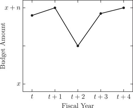
Figure 1 Positive correction.
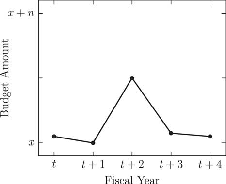
Figure 2 Negative correction.
Figure 2 displays the other prediction of the corrective model, a negative correction. Over the course of the five fiscal years in the figure, the funding level at the start (t) is about the same amount as at the end (t+4) for the programme. In the middle of this budget series is a cluster of punctuations. A positive punctuation occurs at t+2. The financial growth is short-lived, though. A negative budgetary punctuation occurs in the next fiscal year.
In both Figures 1 and 2, the major financial alterations are not sustained over multiple fiscal years. Figure 1 has a one-time funding cut, while Figure 2 has a single influx of money. The corrective model theorizes that budgetary punctuations are temporary shocks to policy systems – budgetary punctuations are not step changes to a new budgetary base level of funding. We theorize it maintains a normal or equilibrium funding level over time. For illustrative purposes, we assume that the corrective punctuations are of the same magnitude as the initial punctuation, though this model can have punctuations that are not fully (or even over) corrective.
We observe these patterns in our dataset of school districts by analyzing our budgetary variable of interest, instructional expenditures per student. For example, a positive correction was observed when a district experienced a drop in instructional expenditures coupled with a rise in enrolment. This drastically reduced the instructional expenditures per student. The next year instructional expenditures were returned to a higher level and total student enrolment had a slight decrease. This was a corrective punctuation back to near the original funding level before the cut.
Budgetary punctuations as trends
The other model we propose is the trending model. This model predicts multi-year punctuations that repeat in either the positive or negative direction. The grouping of punctuations yields a budget that is trending upwards or downwards. This pattern of budgetary punctuations could result from a major change in overall financial resources in a period of several years – economic prosperity can lead to climbing budgets, while hard financial times can shrink funds. Trending budgets could also suggest a reprioritisation of a programme or policy area. Sustained dedication to a programme could yield multiple positive punctuations over several years. Negative budgetary punctuations signal a sustained shift away from a policy, mission or goal of the organisation. New leadership in the organisation could lead to different policy priorities, manifesting as drastic shifts in a programme’s monetary resources – but shifts spread out over several years of implementation. In any of these cases, the financial pattern over time would show a separate clustering of positive and negative punctuations.
The hypotheses for the trending model are:
Hypothesis 3: “Positive Trend.” The probability of a positive budgetary punctuation is positively related to having experienced a positive budgetary punctuation.
Hypothesis 4: “Negative Trend.” The probability of a negative budgetary punctuation is positively related to having experienced a negative budgetary punctuation.
Figures 3 and 4 illustrate each of the hypotheses, similarly to the figures from the corrective model. Figure 3 demonstrates Hypothesis 3, a positive trend. This figure shows how positive budgetary punctuations group together. The budget keeps rising in drastic increments, resulting in a more highly funded programme. On the other hand, Figure 4 displays negative budgetary punctuations over multiple fiscal years. This is referred to as a negative trend in Hypothesis 4. Financial resources for this programme take a massive cut from t to t+4. Overall, these figures show positive budgetary punctuations clustering separately from negative budgetary punctuations.
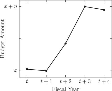
Figure 3 Positive trend.
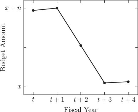
Figure 4 Negative trend.
Unlike the corrective model that portrays budgetary punctuations as shocks to the equilibrium of a programme’s budget, the trending model reveals budgetary punctuations as a path to a new base level of funding. In Figures 1 and 2, the budget returns to a similar level as it began in the series. In Figures 3 and 4, the programme budget adjusts to a new high or low level of funding. For example, in our sample of school districts, a positive trend occurred in the instructional expenditures per student variable for a district that experienced slight declines in enrolment in addition to increases in instructional expenditures. This resulted in much higher funding for instructional expenditures per student in a short timespan of only 2 years.
Data and methods
Data for this study come from one of the most prevalent local governments – school districts. The sample contains budgetary, student and teacher demographic, student performance, and other district level information for Texas school districts from 1993 to 2010. In Texas, there are over 1000 school districts that operate independently, yet maintain the shared goal of educating students. They all share a similar regulatory environment and accounting standards. While school districts must abide by state and federal programme fundings formulas, each school district exercises autonomy over their budgetary decisions. It is a top-down financial process with the school district superintendent and school board making the major budgetary decisions.
The budget of interest in this study is the annual percentage change in instructional expenditures per pupil. Instructional expenditures represent the foremost mission of school districts – educating students. Meier and O’Toole (Reference Meier and O’Toole2009) show that this part of the budget is protected. In comparison to other school functions, it takes a smaller cut when overall financial resources decrease. Alterations in instructional expenditures do not simply follow the health of the economy, but represent choices by school district officials. Furthermore, school district officials have discretion over this part of the budget as opposed to other functions.
The annual percentage change in instructional expenditure per pupil variable is then represented in two dummy variables representing positive and negative punctuations.Footnote 1 A positive punctuation is a budgetary change greater than 35.5%. A negative budgetary punctuation is a budgetary decrease more negative than –33%. The cut points are chosen to stay consistent with previous work (Robinson et al. Reference Robinson, Caver, Meier and O’Toole2007; Robinson et al. Reference Robinson, Flink and King2014). In these studies, the authors determine the cut points for punctuations by overlaying a normal distribution on the histogram of all budgetary changes. The two points of intersection of the histogram and normal curve in the tails of the distribution (above and below the mean of the distribution) are used to mark the point of punctuation. All observations in the tails of the distribution beyond the point of intersection with the histogram are counted as punctuations.Footnote 2
For this study, there are four separate logit models. The first two logit models use positive punctuations as the dependent variable. The last two logit models use negative punctuations as the dependent variable. Both dependent variables are dummy variables indicating the presence of a positive or negative punctuated budgetary change for that year. There are two sets of independent variables. The first set is the 1-year lag of a positive or negative punctuation (two separate dummy variables). Since a 1-year lag is a very narrow timespan, the second set of independent variables widens the window of prior punctuation to 2 years. These are dummy variables indicating if a positive or negative (two unique variables) occurred in the past 2 years.
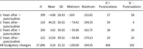
Several other control variables are included in each logit model. To account for organisation performance and personnel stability, the all student standardized test pass rate and teacher turnover were included (Flink Reference Flink2017). Organisation structure was controlled for by the percent of funds spent on centralisation (Robinson et al. Reference Robinson, Caver, Meier and O’Toole2007). Furthermore, the centralisation variable squared was included to account for the declining impact of centralisation (Ryu Reference Ryu2011a). Size of the organisation was controlled for by the number of students enrolled in a district and the enrolment growth rate (annual percentage change in enrolment) (Robinson et al. Reference Robinson, Caver, Meier and O’Toole2007). Additionally, year fixed effects were included in the models. The descriptive statistics are provided in Table 1.
Table 1 Descriptive statistics

Note: N=17,896 for all variables.
It is important to note that these models involve a specific null hypothesis. A lack of evidence for a relationship between past punctuation directions and current punctuation directions would fail to reject a null hypothesis that punctuation directions are unrelated. This null hypothesis contradicts both the corrective and trending models. The statistical significance tests involve a comparison to this null hypothesis rather than a comparison of the evidence for the trending and corrective models. We have retained the null hypothesis of no relationship between direction of change as it is the most common approach to regression hypothesis test and likely to be the default assumption of readers.
Results
Table 1 presents the results for the four logit models. Each of the regressions supports the corrective reactions model of budgetary punctuations. There is no support for the trending model in which budgetary punctuations move consistently upwards or downwards.
Models 1 and 2 utilize positive punctuations as the dependent variable. Model 1 considers how a positive or negative punctuation in the prior year affects the probability of a positive budgetary punctuation. The results show that the presence of a negative punctuation is positive and statistically significant. This means that large budget decreases lead to subsequent budget increases more than one would expect at random. This finding supports Hypothesis 1, positive correction. There is no similar evidence supporting Hypothesis 3 (positive trend); positive budgetary punctuations are not related to having another positive punctuation in the next time period, as suggested in the trending model.
Model 2 examines if a positive or negative punctuation occurred in the previous 2 years. Like Model 1, the 2-year window for negative budgetary punctuations is positively related to positive punctuations and statistically significant. Hypothesis 1 for the corrective model finds more evidence. The 2-year lag for positive punctuations is statistically insignificant. Taking the two models together, there is strong evidence to support the corrective punctuation model – though this alternating sequence does not directly assess the net effect of the two punctuations (a topic we address in the next section).
Models 3 and 4 predict negative budgetary punctuations. Considering a 1-year lag (Model 3), negative punctuations are not correlated with the occurrence of future large negative budgetary changes. This is inconsistent with the negative trend (Hypothesis 4). On the other hand, having a positive budgetary punctuation leads to a higher expected probability of a negative budgetary punctuation in the next year, consistent with Hypothesis 2. Opening up the recent budgetary punctuation window to 2 years, Model 4 shows a similar pattern. Positive punctuations are positive and statistically significant, in line with Hypothesis 2, the negative correction. Negative punctuations have a negative and statistically significant relationship to future negative punctuations. Having a negative punctuation makes it less likely to experience one in the near future – a finding contradicting the trending model. Both Models 3 and 4 support the corrective model of budgetary punctuations. This suggests that punctuations may be equilibrium seeking in the short run.Footnote 3
In both cases (positive and negative punctuations), the results reveal that what could look like a trending pattern disappears once one properly controls for potential confounding variables.
The control variables present interesting findings about how organisational features uniquely contribute to positive and negative punctuations. The (all student) standardized test pass rate is negative and statistically significant across all models. Furthermore, the teacher turnover variable is positive and statistically significant in each of the models. Both of these variables are consistent with the literature that says that higher pass rates and lower turnover will lead to more incremental changes. However, the relationship for each of these variables is much stronger for positive punctuations than negative punctuations.
The impact of centralisation across the four models leads to a curious finding. In Model 1, it is negative and significant. In Model 2, it is insignificant. Centralisation, though, is positive and statistically significant in both Models 3 and 4. These Models demonstrate that organisation centralisation has unique effects for positive and negative punctuations. Centralisation makes positive punctuations less likely, while it improves the odds for more negative punctuations. Centralisation squared is statistically significant and negative in Models 3 and 4, supporting the diminishing impact of centralisation.
Student enrolment, the proxy for organisation size, behaves as expected. The larger the school district, the less likely punctuations are to occur. The relationship between enrolment and expected probabilities of punctuations is negative and statistically significant across models. The effect is stronger on positive punctuations than negative punctuations. The impact of enrolment growth is split by positive and negative punctuations. In Models 1 and 2, high growth leads to lower chances of positive punctuations. The opposite effect is observed in Models 3 and 4 – enrolment growth is more likely to lead to negative punctuations (Table 2).
Table 2 Logit models
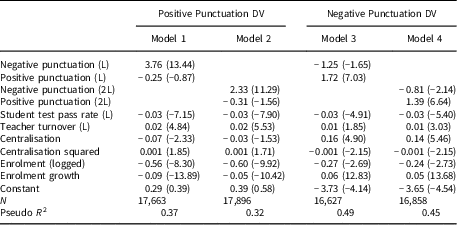
Note. Year fixed effects included in all models. Year 2001 dropped in Models 3 and 4.
Z score in parentheses. L indicates a 1-year lag.
To visually illustrate the results of the logit models, simulationsFootnote 4 of the probability of experiencing positive and negative punctuations that are shown in Figure 5. All variables are held to their means except for the previous punctuation variables, which are alternated between 1 and 0. The probability of a positive/negative punctuation is shown with experiencing a positive or negative punctuation in the previous 1- or 2-year window, depending on the model. The effect of a previous negative punctuation is the solid line while the effect of a previous positive punctuation is the dashed line.
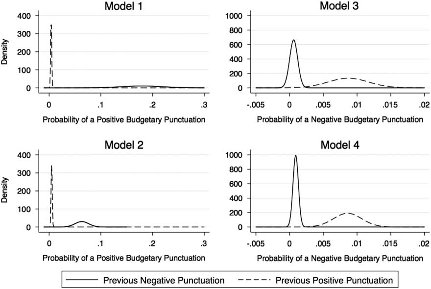
Figure 5 Effect of prior year punctuation on current punctuation.
The distributions of Figure 5 illustrate the pattern expected in the corrective model. Overall, Figure 5 illustrates how the direction of the previous punctuation significantly changes the probability of future punctuations. In Model 1, a previous negative punctuation increases the probability of a positive punctuation to 17%. Compared to a previous positive punctuation, which is near zero, this is a drastic increase in probability. Model 2 illustrates the same relationship (the probability of a positive punctuation conditioned in the direction of prior punctuations) as Model 1 – but with a 2-year window. Models 3 and 4 are consistent with the pattern in Models 1 and 2 supporting the corrective model with a 1- and 2-year window of prior punctuations. There are only small differences in the probability distributions between these two models.
Budgetary changes following punctuations
The logit models suggest that punctuations may be equilibrium seeking with large changes leading to immediate large changes in the opposite direction. Figures 1 and 2 of the corrective model assumed that the corrective punctuation was of the same magnitude as the initial punctuation. This was just an assumption for illustrative purposes. The models in the previous section displayed the sequence of the punctuation direction (alternating directions) but did not directly assess the magnitudes of the two punctuations.
The magnitude of the changes can signal important differences in the underlying process. If the magnitudes of the alternating punctuations are similar, this may be a process in which the punctuations do not have lasting effects – even 2 years later. On the other hand, if the second punctuation is typically smaller than the first, some proportion of the changes will persist.
To compare the magnitude of alternating punctuations, we assessed the subsample of punctuations that follow this alternating pattern.
In the first set, the distributions of budgetary changes are shown for 1 year and 2 years immediately following both positive and negative punctuations. These distributions reveal if shifts (left or right) occur in light of massive budgetary changes. For positive punctuations, negative punctuations are expected, per the logit models. However, if budgets claw back in slightly smaller increments, we should see a cluster of observations around negative, medium budgetary changes. The same holds true for negative punctuations – positive punctuations and medium changes should hold more observations in the distribution. Any clustering around 0% means the budgetary change was retained.
Another set of distributions reveal whether short-run budgetary equilibria are kept. In particular, distributions immediately following a pair of punctuations (one positive and one negative) illustrate whether the budget returns to its original level. Equilibrium seeking punctuated behavior occurs when these distributions cluster around the zero mark.
Distribution of budgetary changes
How do budgets respond after a punctuation? The empirical models in the previous section show that punctuations lead to more punctuations. The comparison of the magnitude of the punctuations reveals more about the dynamics of sequential punctuations.
The corrective model suggests big moves in one direction (positive or negative) leads to more changes (of any size) in the other direction. The distributions are expected to illustrate this by having a number of punctuations in the opposite direction of the previous punctuation. Furthermore, the distribution should be shifted towards the opposite direction of the punctuation – more observations should be observed in the medium size changes as well. A tall central peak centred at zero in the distribution means that the punctuation level was kept – the next fiscal period did not work to correct the punctuation.
Table 3 reports a three-by-three table of the categories of punctuations (none, positive, negative) for year t−1 and year t. By the numbers, it is observed that positive punctuations in t−1 yield negative punctuations 14.5% of the time compared to another positive punctuation 6.8% of the time. The most common occurrence though is a single positive punctuation at 78.7%. For negative punctuations in t−1, positive punctuations occur 49.6% of the time in response, while negative punctuations occur 3.4%. Negative punctuations are followed by no punctuation at 47.1% of the time. This illustrates that even among the raw numbers of the categorical variables, the corrective model is supported in positive versus negative punctuations.
Table 3 Categories of punctuations in time t−1 and time t
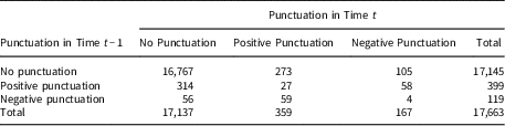
Table 4 and Figure 6 examine the distribution of budgetary changes and descriptive statistics 1 year and 2 years after a positive and negative punctuations. The patterns provide context for the statistical model. In the year following a punctuation, the mean values of budgetary changes are altered from the mean of all budgetary changes, around 4%. One year after a positive punctuation, the mean shifts down to negative 4% – a modest change of 8%. In a more drastic shift, 1 year after a negative punctuation, the mean budgetary change is 44%. Considering all of Figure 6, second punctuations are more likely than the initial ones, but they are still relatively rare. Instead, a punctuation leads to a shift in the mean and a widened range of budgetary changes – largely mirroring the overall distribution of budgetary changes.
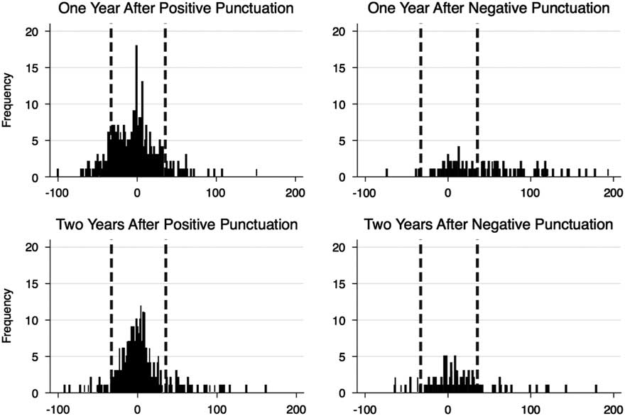
Figure 6 Annual per cent budgetary change after punctuations.
Table 4 Annual per cent budgetary change after punctuations
Another interesting result in Figure 6 is that the distributions after positive punctuations seem to cluster around zero and in the shoulders of the distribution more than the negative punctuation distributions. This illustrates that a greater portion of the positive budgetary changes are being retained for some time. The negative budgetary punctuations lead to distributions that are more of uniform shape than a normal distribution.
Lastly, it is interesting that most corrective punctuations are occurring in the year after the punctuation, as opposed to 2 years after the punctuation. This is evident by Figure 6 – there are many more observations of punctuations in the top row than the bottom row. This tells us that corrections are immediate.
Corrective punctuations
Given the similarity of the postpunctuation distribution of budgetary changes, it is important to assess the degree to which punctuations are fully “corrected” by the compensating changes. Are the second punctuations of similar sizes to the original punctuations? This could be an indication that the punctuations are temporary exceptions in an equilibrium seeking system. In a strong version, an equilibrium seeking system would react to a punctuation with an equal and opposite budgetary change – resulting in no net change in the budget. This is the model illustrated in Figures 1 and 2. The data allow us to directly assess the extent to which punctuations are “corrected” to their original budget by the corrective punctuation pattern.
Table 4 and Figure 7 present the results for this assessment. It is important to keep in mind that out of the hundreds of punctuations, only 59 and 58 follow the alternating pattern. While this represents more secondary punctuations than one would expect if there were no relationship between punctuation propensity, these are still rare events – even rare in the context of punctuated change. We are discussing 117 instances of paired punctuations out of the 600 total punctuations.
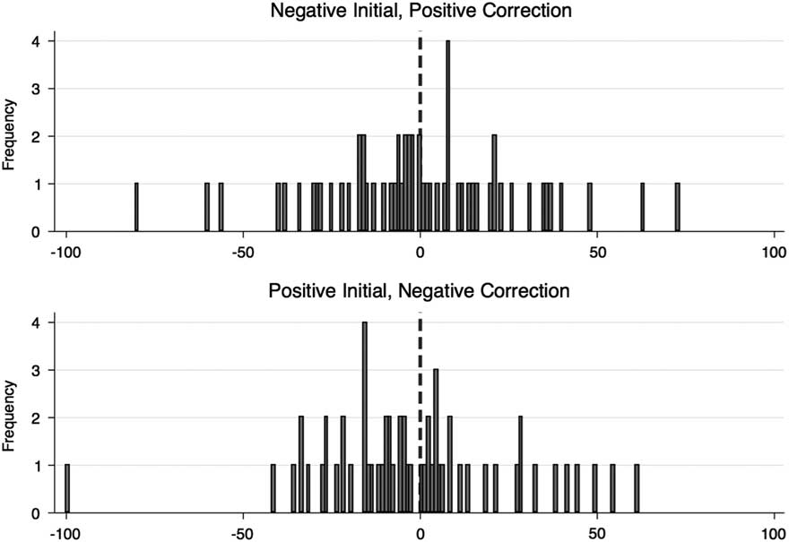
Figure 7 New budget’s per cent of original budget.
Figure 7 shows the percentage of budgetary change from the original budget level (before punctuations) to the level after two punctuations (initial and corrective, positive and negative). A score at 0% means that the budget was returned to its original level – the punctuations were perfectly corrective. A score in the negatives means that the new budget level is less than the amount before punctuations. A positive budgetary change means that the punctuations resulted in a higher budget than before the punctuations (Table 5).
Table 5 New budget’s per cent of original budget
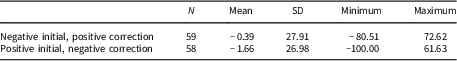
The information on Table 4 suggests that second punctuations are, on average, fully corrective. The net result of a negative-then-positive pair is a reduction of a mere 0.39% in the budget. This is effectively a full correction. However, the mean conceals a great deal of variation around that mean. The distribution (illustrated on the top half of Figure 7) is almost uniformly distributed around the mean with a range from –80% to 73% and a SD of 28. While the average pair is corrective, the average value is not as likely an observation in these data with a more uniform shape, as compared to a normal distribution.
The same pattern appears in positive-then-negative pairs. The net change of these pairs is, on average, a reduction of 1.66%. This is not as close to zero as the other alternating pair, but still a small net change. Again the distribution has a large standard deviation (27) with a remarkable range around this mean – with the negative side of the distribution weighed down by a single observation at a complete net reduction of the budget (–100%). In both cases, the compensatory nature of paired punctuations is accurate on average but conceals a great deal of variation in these budgetary systems.
Conclusion
Research has shown that budgetary punctuations in public organisations happen in groupings over time. The direction of those budgetary changes – positive or negative – has not been examined by scholars. The purpose of this study was to test two models of the sequence of budgetary punctuations: the corrective model and the trending model. In the corrective model, positive and negative punctuations cluster together; large movement in one direction is responded to by a punctuation in the opposite direction. In the trending model, positive punctuations lead to more positive punctuations and negative punctuations lead to more large budgetary decreases.
In an examination of hundreds of Texas school districts over an 18-year period, the corrective model is consistent with the data.Footnote 5 Of the four hypotheses, Hypothesis 1 (positive correction) and Hypothesis 2 (negative correction) were supported in each of the logit models predicting positive and negative budgetary punctuations. For practitioners, this means large budget increases are generally short-lived (according to our multivariate model in Table 2), so they must be exploited to their fullest potential. On the other hand, large budget decreases are also likely to be followed by a significant budget increase. Managers must endure substantial budget cuts for only a short time.
The distributional analyses brought deeper understanding to budgetary changes following punctuations. More than just punctuations in the opposing direction, the distribution shifts to more medium size changes in the opposite direction as well after a budgetary punctuation. Also, the distributions showed how the positive/negative punctuation pairs did not always result in a short-term equilibrium point. While the mean budgetary change after two punctuations was near zero, suggesting a full correction from the following punctuation, the standard deviation was large. This brings a nuanced understanding to the logit models on predicting the occurrence and response to punctuations.
For the PET literature, these findings provide further insight into not just predicting when budgetary punctuations occur, but the direction of the budgetary change. It offers more specific predictions on the dynamics of the policy process. In the public budgeting literature, these findings help scholars to understand the movement of budgets. Specifically, it provides new insights into when major financial changes occur.
The results illustrate the (incompletely) corrective nature of many punctuations. This opens the question of when permanent large changes occur rather than a largely corrected short-term large change. The period of punctuation – once a punctuation has occurred but before a new equilibrium is fully in place – emerges as an important target of investigation for scholars of budgetary change.
It is natural to consider the extent to which these patterns would hold in other institutional settings. The evidence here can only speak to education policymaking. However, the success of replicating previous results in education setting to other settings – including federal and state budgetary processes (Ryu Reference Ryu2011a). Other settings may also provide useful opportunities to consider the completeness of corrective punctuation pairs.
The results suggest the importance of more careful consideration of the dynamics of change within periods of punctuation – rather than thinking of punctuations as merely discrete events. Given the commonality (though not universality) of corrective punctuations, policy theorists should consider the conditions when we will see alternating, corrective actions rather than last changes. Theorising along these lines will return the literature to its roots in assessments of the conditions under which genetic variation would increase dramatically within a geological era.
There are also interesting implications for budgetary dynamics outside of the context of PET. The results spotlight the clustering of compensating budgetary changes. Within budgetary theories, what does this suggest about political or organisational forces that shape these budgetary changes? These results open questions specific to budgetary processes beyond those bounded by the context of PET.
Future research can examine other determinants of budgetary punctuations. For one, the control variables in this work suggested interesting findings in how organisational features uniquely lead to more positive or negative punctuations. More work can be done to determine what characteristics affect how organisations can more easily process negative or positive budgetary changes.
The management or leadership dimensions can be further explored as well. Do rapid policy changes occur at the beginning of a manager’s leadership tenure demonstrating an organisation’s willingness to embrace new leadership? Or, do rapid policy changes take place later in a manager’s tenure once he/she has learned the workings of the organisation and control their surroundings? There are many avenues of research in understanding dynamic budgeting in public organisations and institutions.
Supplementary materials
To view supplementary material for this article, please visit https://doi.org/10.1017/S0143814X18000259
Data
Replication materials are available at https://dataverse.harvard.edu/dataset.xhtml?persistentId=doi:10.7910/DVN/SBVFUL.
Acknowledgements
We thank the Editor and Reviewers for their thoughtful comments.


