


1. Introduction
The oblique interaction of solitary waves or solitons is a fundamental problem in fluid dynamics and nonlinear sciences more broadly. Early theoretical consideration of this problem for acute, collisional angles of incidence dates back to Miles (Reference Miles1977a,Reference Milesb), where weak and strong gravity water wave soliton interactions were shown to be dependent upon the incidence angle and soliton amplitudes. In the case of weakly interacting oblique solitons, a sufficiently small incidence angle leads to the approximate linear superposition of the two solitons accompanied by a phase shift. The strong interaction case at large acute angles leads to a resonant triad of obliquely interacting solitary waves, the so-called Miles resonant soliton. Miles used his theory to identify the long-time dynamics of regular and Mach reflection of a soliton incident upon a compressive corner or wedge.
Building upon original water wave experiments by Perroud (Reference Perroud1957), Miles’ studies have since been expanded and refined with the help of laboratory experiment (Melville Reference Melville1980; Li, Yeh & Kodama Reference Li, Yeh and Kodama2011; Kodama & Yeh Reference Kodama and Yeh2016) and field observations (Ablowitz & Baldwin Reference Ablowitz and Baldwin2012; Wang & Pawlowicz Reference Wang and Pawlowicz2012), numerical simulation (Funakoshi Reference Funakoshi1980; Tanaka Reference Tanaka1993; Porubov et al. Reference Porubov, Tsuji, Lavrentov and Oikawa2005; Tsuji & Oikawa Reference Tsuji and Oikawa2007; Biondini et al. Reference Biondini, Maruno, Oikawa and Tsuji2009; Kodama, Oikawa & Tsuji Reference Kodama, Oikawa and Tsuji2009; Li et al. Reference Li, Yeh and Kodama2011; Kao & Kodama Reference Kao and Kodama2012; Chakravarty, McDowell & Osborne Reference Chakravarty, McDowell and Osborne2017) and exact multisoliton solutions (Kodama Reference Kodama2004; Biondini Reference Biondini2007; Biondini et al. Reference Biondini, Maruno, Oikawa and Tsuji2009; Chakravarty & Kodama Reference Chakravarty and Kodama2009; Kodama Reference Kodama2010; Kodama & Yeh Reference Kodama and Yeh2016) of the Kadomtsev–Petviashvili (KP) equation and its higher-order generalisations. The KP equation is a generic model of weakly nonlinear, weakly dispersive unidirectional waves with weak transverse variation (Kadomtsev & Petviashvili Reference Kadomtsev and Petviashvili1970)
 \begin{equation} (u_t + uu_x + u_{xxx})_x + u_{yy} = 0, \quad (x,y) \in \mathbb{R}^{2}, \quad t > 0, \end{equation}
originally derived in the context of shallow water waves by Ablowitz & Segur (Reference Ablowitz and Segur1979) and for internal waves by Grimshaw (Reference Grimshaw1981). Subscripts in (1.1) and elsewhere correspond to partial derivatives. In applications such as shallow water waves, the non-dimensionalisation is achieved by entering the reference frame moving with the long wave speed  $\sqrt {gh}$ (
 $g$ is gravitational acceleration and
  $h$ is the mean fluid depth), scaling time by
  $\tau$, scaling the longitudinal and transverse lengths by the typical wavelengths
  $\lambda _x$ and
  $\lambda _y$, respectively, and scaling the surface disturbance height by the typical amplitude
  $\eta$. The KP equation arises when weak nonlinearity, long wave dispersion and weak transverse variation balance according to, respectively,
  $\eta /h \sim (h/\lambda _x)^{2} \sim (\lambda _x/\lambda _y)^{2} \ll 1$. The particular scaling in (1.1) manifests if we set
  $\tau = \lambda _x^{3}/(h^{2}\sqrt {gh})$,
  $\lambda _y = \lambda _x^{2}/(\sqrt {2}h)$, and
  $\eta = 2 h^{3}/(3\lambda _x^{2})$ for some
  $\lambda _x \gg h$. The asymptotic validity of the KP equation requires small transverse wave curvature for quantitative comparison with physical observations. Geometric and higher-order asymptotic considerations can be used to achieve even better agreement between theory and experiment (Kodama & Yeh Reference Kodama and Yeh2016).
This version of the Kadomtsev–Petviashvili equation is known as the KPII equation – the KPI equation occurs when  $+u_{yy} \to -u_{yy}$. The KPII equation is a completely integrable equation (Ablowitz & Clarkson Reference Ablowitz and Clarkson1991) that admits a two-parameter family of stable line soliton solutions
 \begin{equation} u(x,y,t) = a \,\mathrm{sech}^{2}\left(\sqrt{\frac{a}{12}}(x + q y - ct)\right), \quad c=\frac{a}{3}+q^{2} , \end{equation}
uniquely determined by the amplitude  $a > 0$ and soliton inclination from the
  $y$-axis or slope
  $q \in \mathbb {R}$. See figure 1 for a representative example. We note that the weak transverse scaling used in the derivation of the KP equation (1.1) incorporates this assumption so that the slope
  $q$ can be an order-one quantity.

Figure 1. Contour plot of a line soliton solution and its slope parametrisation. The soliton propagation slope is  $q = \tan \varphi$.
The Mach reflection problem has an interesting history that begins with Ernst Mach's research on shock wave interactions in gas dynamics. Utilising two separated electric spark sources between two glass plates, one covered in soot, Mach & Wosyka (Reference Mach and Wosyka1875) generated cylindrical shock fronts that left residual patterns from their interaction. From these experiments, Mach keenly discerned two types of shock interaction – termed regular and irregular – that depended upon the interacting fronts’ obliqueness. Both cases involved a reflected shock but the irregular interaction for sufficient obliqueness resulted in a triple point where three regions of different pressures and densities met. An additional wave was generated from the triple point and has become known as the Mach stem resulting from Mach reflection of shock waves (Krehl & van der Geest Reference Krehl and van der Geest1991). Motivated by the so-called hydraulic analogy between two-dimensional supersonic gas dynamics and supercritical shallow water waves, Gilmore, Plesset & Crossley (Reference Gilmore, Plesset and Crossley1950) reconsidered regular and Mach reflection of shocks by obliquely interacting two hydraulic jumps. This phenomenon was also observed in shallow ocean waves (Cornish Reference Cornish1910). But the theoretical interpretation of Mach reflection in water waves had to wait until the seminal work of Miles (Reference Miles1977a,Reference Milesb), in which two obliquely interacting solitary waves were described. The irregular or Mach reflection case is embodied in the resonant or  $Y$-shaped solitary wave solution. Regular reflection is described by the
  $X$-shaped solitary wave solution. Regular and Mach reflection can also be formulated as an initial-boundary value problem in which a semi-infinite shock or soliton propagating parallel to a wall impinges upon a wedge or corner. Depending upon the corner angle, the ensuing dynamics leads to the spontaneous generation of a reflected wave and, in the case of irregular or Mach reflection, the additional generation of a Mach or stem wave in which a resonant triad of three waves meet and propagate away from the wall. See figure 2 for a schematic of the two reflection types. Because the KP equation (1.1) is a generic, universal model of weakly nonlinear, dispersive, two-dimensional wave patterns, regular and Mach reflection are fundamental to the description of multidimensional nonlinear waves.

Figure 2. Schematic of Mach (a) and regular (b) reflection of a soliton impinging upon a compressive corner.
One approach to describe Mach reflection of solitons is the use of exact solutions of the KPII equation (Li et al. Reference Li, Yeh and Kodama2011). A classification of 2-soliton solutions in (Kodama Reference Kodama2004; Biondini Reference Biondini2007; Chakravarty & Kodama Reference Chakravarty and Kodama2009) was used to identify two particular 2-soliton solutions whose parameters can be chosen to satisfy the requisite structure of regular and Mach reflected waves. To describe the soliton-corner initial-boundary value problem, a nonlinear method of images is applied and hypothesised to locally describe the long-time dynamics. This results in the critical angle  $\varphi _{cr}$ – corner inclination measured from the positive
  $x$-axis – for the transition from regular,
  $\varphi > \varphi _{cr}$, to Mach,
  $0 < \varphi < \varphi _{cr}$, reflection of an incident soliton with amplitude
  $a$ as
 \begin{equation} \tan{\varphi_{cr}} = \sqrt{a}. \end{equation}
Numerical simulations of initially V-shaped waves were used to justify the long-time, locally 2-soliton solution hypothesis for the soliton-corner initial-boundary value problem (Kodama et al. Reference Kodama, Oikawa and Tsuji2009; Kao & Kodama Reference Kao and Kodama2012). Herein lies a subtle difference between oblique soliton interaction – described by exact 2-soliton solutions – and a soliton incident upon a corner, which involves a transient dynamics that, after long enough times, is locally described by 2-soliton solutions.
The aforementioned regular/Mach reflection problem involves a compressive corner with angle  $\varphi$ measured counterclockwise from the positive
  $x$-axis. In this paper, we consider the problem of a soliton incident upon an expansive corner, opening in the opposite direction so that
  $\varphi$ is measured clockwise from the positive
  $x$-axis. This problem is rather different from the regular/Mach reflection problem in many respects but we find an interesting parallel. The critical corner angle that separates regular expansion and Mach expansion for an incident soliton with amplitude
  $a$ occurs precisely at
  $\varphi _{cr}$, the same critical angle separating regular and Mach reflection in (1.3). Regular expansion occurs when
  $\varphi > \varphi _{cr}$ and leads to the development of a decaying parabolic wave that connects the incident soliton to the wall. Mach expansion when
  $0 < \varphi < \varphi _{cr}$ involves the development of a new soliton perpendicular to the wall with reduced amplitude relative to the incident soliton. The development of this soliton is the expansion analogue of the Mach stem in the reflection case. See figure 3 for a schematic of the two cases.

Figure 3. (a,c) Diagram of Mach expansion for a front encountering a reverse wedge boundary with small  $\varphi$ (a,b) and large
  $\varphi$ (c,d). Note the emergence of a new, smaller amplitude line soliton along the boundary when
  $\varphi$ is small. (b,d) Bent soliton initial conditions are identical for the purposes of analysis.
A new approach is required to describe regular and Mach expansion of solitons because the dynamics is not described by multisoliton solutions. While the transient dynamics of Mach reflection is subtle, crucial aspects of Mach expansion are transient and are not steady in a local reference frame. By making a slowly varying assumption, we approximately describe the full expansion dynamics developing from initial value problems by appropriate modulation of the line soliton (1.2a,b). Our KPII numerical simulations demonstrate that modulation theory is effective at uncovering key, quantitative features of the nonlinear wave dynamics.
In order to describe the soliton-corner expansion problem, we take a seemingly circuitous route by considering three classes of initial value problems, depicted in figure 4, for the KPII equation (1.1). From left to right, we identify the data as truncated, bent-stem and bent soliton initial conditions. The bent soliton case corresponds to the appropriate reflection, via the nonlinear method of images (Kodama & Yeh Reference Kodama and Yeh2016), needed to describe regular/Mach expansion as depicted in figure 3. Bent initial conditions are equivalent to a single soliton moving along a boundary at the location where the boundary suddenly angles away from the front.

Figure 4. Initial data corresponding to a truncated line soliton (a), a bent-stem soliton (b) and a bent soliton (c).
The reason for considering these three classes of initial data in turn is both mathematical and physical. From a mathematical point of view, each initial condition limits to the next so that their solution is informed by the previous and they share some solution properties. Moreover, these are among the simplest and more natural kinds of non-solitonic initial conditions for the KP equation one could consider. Although the data consist of modulated solitons, they do not contain exact soliton solutions. In contrast to our approach, the primary analytical means by which all previous studies have interpreted related non-solitonic initial value problems is by approximating the evolution of initial configurations with exact multisoliton solutions of the KP equation. See, for example Biondini et al. (Reference Biondini, Maruno, Oikawa and Tsuji2009), Kao & Kodama (Reference Kao and Kodama2012) and Chakravarty et al. (Reference Chakravarty, McDowell and Osborne2017).
From a physical point of view, the truncated soliton initial data models the emergence of a quasi-one-dimensional soliton from transverse confinement such as the internal ocean solitons generated at the front of a river plume (Nash & Moum Reference Nash and Moum2005; Pan, Jay & Orton Reference Pan, Jay and Orton2007; Wang & Pawlowicz Reference Wang and Pawlowicz2017) and a surface wave soliton when a channel suddenly widens. This problem was considered experimentally by John Scott Russell in his celebrated Report on Waves (Russell Reference Russell1845). The rapid deceleration or transcritical propagation of a ship in open, shallow water can similarly launch a bent-stem or bent soliton from the ship's prow (Li & Sclavounos Reference Li and Sclavounos2002), dependent upon the prow shape. Finally, internal wave solitons are ubiquitous in the world's oceans (Jackson Reference Jackson2004; Wang & Pawlowicz Reference Wang and Pawlowicz2012) and topography significantly impacts their propagation and interaction (Yuan et al. Reference Yuan, Grimshaw, Johnson and Wang2018). The classes of initial data in figure 4 represent cases where the modulated solitons propagate away from one another. Nevertheless, their interaction is significant.
We study these initial value problems using modulation theory in which the local soliton amplitude  $a = a(y,t)$ and slope
  $q = q(y,t)$ are allowed to vary slowly in space and time. There are several approaches to derive the effective modulation equations. In appendix A, we provide a derivation using multiple scale perturbation theory of the equations
 \begin{gather} a_t + 2 q a_y + \tfrac{4}{3} a q_y = 0, \end{gather}
 \begin{gather}q_t + 2 q q_y + \tfrac{1}{3} a_y = 0 . \end{gather}
The dynamical equation (1.4a) for the amplitude results from an appropriate orthogonality condition and the slope equation (1.4b) results from a consistency condition of the modulated phase. The modulation equations (1.4) were also derived from a variable coefficient KP equation in (Lee & Grimshaw Reference Lee and Grimshaw1990) and by an averaged Lagrangian approach in Neu (Reference Neu2015) and Grava, Klein & Pitton (Reference Grava, Klein and Pitton2018). They are also a limiting case of the more general KP–Whitham modulation equations for periodic waves (Ablowitz, Biondini & Wang Reference Ablowitz, Biondini and Wang2017) in the case of  $x$ independent modulations of a line soliton (Biondini, Hoefer & Moro Reference Biondini, Hoefer and Moro2020). These soliton modulation equations are equivalent to the equations modelling the isentropic flow of a polytropic gas with density
  $\propto a^{3/2}$, velocity
  $\propto q$ and ratio of specific heats
  $\gamma = 5/3$. The linearisation of the modulation equations (1.4) for small
  $|q|$ was used in Kadomtsev and Petviashvili's original paper to determine the stability of line soliton solutions to the KP equation (Kadomtsev & Petviashvili Reference Kadomtsev and Petviashvili1970).
Despite variation in only one spatial dimension, the corresponding modulated line solitons exhibit non-trivial two-dimensional structure. In particular, once a modulation solution  $a(y,t)$,
  $q(y,t)$ is obtained, the modulated soliton is reconstructed by projection onto (1.2a,b) according to
 \begin{equation} \left.\begin{gathered} u(x,y,t) \sim a(y,t) \,\mathrm{sech}^{2}\left ( \sqrt{\frac{a(y,t)}{12}} \xi \right ), \\ \xi = x + \int_0^{y} q(y',t)\,\mathrm{d} y' - \int_0^{t} c(0,t')\,\mathrm{d} t' , \end{gathered}\right\} \end{equation}
where the soliton speed satisfies  $c(y,t) = a(y,t)/3 + q(y,t)^{2} = -\xi _t(x,y,t)$ (cf. (1.2a,b) and (A 3)).
The class of initial data we consider here corresponds to expansive conditions, so that we are guaranteed global existence of modulation solutions. We will obtain explicit modulation solutions in the form of simple waves and their interactions that describe the evolution of the data shown in figure 4.
Our analysis is supported by numerical simulations of the KPII equation (1.1) using a Fourier pseudospectral method adapted from Kao & Kodama (Reference Kao and Kodama2012) that allows for outgoing line solitons at the top and bottom of the simulation domain  $[-L_x,L_x]\times [-L_y,L_y]$ through use of a windowing function. We maintain the non-local constraint
  $\int _{-L_x}^{L_x} u_{yy}\,\mathrm {d} x = 0$ to high accuracy by including localised ‘image’ initial data whose superposition with the test data of interest satisfies this constraint. Simulations were terminated before the image and test data interacted. For further details, see appendix B.
2. Basic properties of the modulation equations
In this section, we summarise the classical analysis of the hyperbolic system (1.4).
The modulation equations admit the amplitude symmetry
 \begin{equation} a' = a/A, \quad q' = q/\sqrt{A}, \quad y' = \sqrt{A} y, \quad t' = t, \quad A > 0 , \end{equation}
the quasi-rotational symmetry
 \begin{equation} a' = a, \quad q' = q + Q, \quad y' = y - 2Q t, \quad t' = t, \quad Q\in \mathbb{R}, \end{equation}
the hydrodynamic scaling symmetry
 \begin{equation} y' = \alpha y, \quad t' = \alpha t, \quad \alpha > 0, \end{equation}
and the reflection symmetry
 \begin{equation} y' = -y, \quad q' = -q , \end{equation}
all leaving (1.4) unchanged in primed coordinates. Namely, if  $a(y,t)$ and
  $q(y,t)$ solve (1.4), so do
  $a'(y',t')$ and
  $q'(y',t')$.
It was shown in Biondini et al. (Reference Biondini, Hoefer and Moro2020) that appropriate linear combinations of (1.4a) and (1.4b) result in the equivalent pair of equations in characteristic form
 \begin{equation} \pm \left [ a_t + (2q \pm \tfrac{2}{3}\sqrt{a})a_y\right ] + 2 \sqrt{a} \left [ q_t + (2q \pm \tfrac{2}{3}\sqrt{a})q_y\right ] = 0, \end{equation}
which reveal the characteristic velocities  $U = 2q - \frac {2}{3} \sqrt {a}$ and
  $V = 2q + \frac {2}{3} \sqrt {a}$. Integration of (2.2) along each characteristic direction demonstrates that
 \begin{equation} r = q - \sqrt{a}, \quad s = q + \sqrt{a} \end{equation}
are Riemann invariants for the modulation equations (1.4), which afford the diagonalisation
 \begin{gather} r_t + U r_y = 0, \quad s_t + V s_y = 0, \end{gather}
 \begin{gather}U = \tfrac{2}{3}(2r + s), \quad V = \tfrac{2}{3}(r + 2s) , \end{gather}
where the characteristic velocities  $U$ and
  $V$ are now written in terms of the Riemann variables
  $r$ and
  $s$.
$s$.
Simple wave solutions of (2.4) correspond to variation in only one characteristic direction so that one of the Riemann invariants  $r$ or
  $s$ is constant, i.e. either
  $q(y,t) + \sqrt {a(y,t)}$ or
  $q(y,t) - \sqrt {a(y,t)}$ is independent of
  $y$ and
  $t$. Since the characteristic velocities are ordered
  $U \leqslant V$, we identify simple waves with variation along the slow characteristics
  $\mathrm {d} x/\mathrm {d}t = U$ as 1-waves (
 $s = \textrm {const}$) and those with variation along the fast characteristics
  $\mathrm {d} x/\mathrm {d}t = V$ as 2-waves (
 $r = \textrm {const}$). Across a simple wave, the non-constant Riemann invariant's characteristic velocity is monotonically increasing because the strictly hyperbolic system (1.4) is genuinely nonlinear so long as
  $a > 0$ (Biondini et al. Reference Biondini, Hoefer and Moro2020).
Expansive initial data  $a(y,0)$,
  $q(y,0)$ correspond to the condition that both characteristic velocities
  $U$ and
  $V$ evaluated on the initial data are monotonically increasing functions of
  $y$. By virtue of the fact that
  $\partial U/\partial r = \partial V/\partial s = \frac {4}{3} > 0$, expansive initial data correspond to the case where both Riemann invariants
  $r$ and
  $s$ are non-decreasing functions of
  $y$.
$y$.
Simple waves propagate into constant regions of the  $y$–
$y$– $t$ plane, and are therefore fundamental building blocks for Riemann problems that posit step initial data at the origin. The interaction of simple waves can most conveniently be investigated by use of the hodograph transformation (Courant & Friedrichs Reference Courant and Friedrichs1948) in which the role of dependent and independent variables is swapped. Namely, we take
  $t = t(r,s)$,
  $y = y(r,s)$, yielding the following set of linear equations
 \begin{gather} t_{rs} + \frac{2}{s-r}(t_r - t_s) = 0, \end{gather}
 \begin{gather}y_s = U t_s , \quad y_r = V t_r, \end{gather}
so long as the Jacobian  $J = r_t s_y - s_t r_y$ remains non-zero. Equation (2.5a) is an Euler–Poisson–Darboux (EPD) equation that is equivalent to the radial wave equation in five dimensions, which admits the general solution
 \begin{equation} t(r,s) = A + \left ( \frac{F(r)}{(s-r)^{2}} \right )_r + \left ( \frac{G(s)}{(s-r)^{2}} \right )_s , \end{equation}
for an arbitrary constant  $A \in \mathbb {R}$ and functions
  $F(r)$,
  $G(s)$. In order to determine
  $A$,
$A$,  $F$ and
  $G$, one must specify suitable initial and/or boundary conditions.
3. Partial and truncated line solitons
By a partial or truncated line soliton, we mean initial data in which the soliton modulation amplitude is zero on one or two semi-infinite intervals, respectively. This scenario where  $a = 0$ corresponds to a vacuum state in which the soliton slope
  $q$ is undefined. To resolve this ambiguity, we will require that the value of
  $q$ in the neighbourhood of the point where
  $a$ becomes positive corresponds to a simple wave in which one of
  $r$ or
  $s$ is constant (Smoller Reference Smoller1994). Then, the propagation speed of the vacuum front will necessarily be
  $\lim _{a\to 0} U = \lim _{a\to 0} V = 2q$.
3.1. Partial line solitons
This problem was previously posed and solved in Neu (Reference Neu2015) as a model for two-dimensional soliton diffraction or diffusion as identified by Russell (Reference Russell1845). Here, we show that the resulting simple wave solution forms an important building block for other, more complex, truncated and partial soliton interactions.
Without loss of generality (recall the symmetries (2.1)), we consider the partial (half) line soliton initial data
 \begin{equation} a(y,0) = \begin{cases} 0, & y > 0, \\ 1, & y \leqslant 0, \end{cases} \quad q(y,0) = 0, \quad y < 0, \end{equation}
for the modulation equations (1.4). This Riemann problem is solved by a 1-wave corresponding to a centred, self-similar rarefaction wave (1-RW) in which  $s = q+\sqrt {a} \equiv 1$ and
  $U = y/t$ (Neu Reference Neu2015)
 \begin{equation} \sqrt{a_{p}(y,t)} = \begin{cases} 0, & 2t < y, \\ \frac{3}{4} ( 1- {y}/({2t})), & -\frac{2}{3} t < y < 2t \\ 1, & y < -\frac{2}{3} t, \end{cases}, \quad q_{p}(y,t) = 1 - \sqrt{a_{p}(y,t)} . \end{equation}
This solution describes the progressive disintegration of the partial soliton. This evolution is shown in figure 5(a–c), where we depict the evolution of the partial soliton, as computed via numerical integration of the KP equation (see appendix B). In figure 5(d,e), we compare the analytical predictions with numerical evolution by identifying the positions of the vacuum front and vertical soliton front as the first points where  $a \to 0.03$ and
  $a \to 0.97$, respectively. These fronts are well approximated by straight lines with slopes given by the predicted characteristic speeds from the solution in (3.2). Below, we will use the solution in (3.2) to analyse the evolution resulting from more complex initial conditions.

Figure 5. (a–c) Numerical simulation of partial soliton evolution for  $t \in (0,60,300)$. (d,e) Comparison of characteristic speeds of the upper (d) and lower (e) edges of the partial soliton rarefaction wave. The plot displays the predicted front speeds as reference lines (dash-dotted, blue) with slopes from the solution (3.2), the numerically extracted front positions (solid, black) and a least squares linear fit (dashed, red) whose slope determines the measured speeds.
3.2. Truncated line solitons
We now consider the KPII equation with initial conditions for a truncated line soliton (recall figure 4a) of length  $\ell > 0$ by imposing the modulation initial conditions
 \begin{equation} a(y,0)= \begin{cases} 1, & |y| \leqslant \ell/2, \\ 0, & |y| > \ell/2, \end{cases} \quad q(y,0)= 0, \quad |y| < \ell/2 . \end{equation}
By the reflection symmetry (2.1d),  $q$ and
  $a$ are respectively odd and even functions of
  $y$ for each
  $t \geqslant 0$. As in the case of the partial soliton, the truncated soliton slope in the vacuum region where
  $a = 0$ is determined by a simple wave condition. Namely, for short times, a non-centred 1-RW is generated from the upper truncation point at
  $y = \ell /2$. Similarly, a 2-RW is generated from the lower truncation point
  $y = -\ell /2$. By use of the reflection symmetry (2.1d), the initial evolution of these two simple waves can be represented as even or odd extensions of a shifted partial soliton (3.2)
 \begin{equation} a(y,t) = a_{p}(|y|-\ell/2,t), \quad q(y,t) = \mathrm{sgn}(y)q_{p}(|y|-\ell/2,t), \end{equation}
for  $y \in \mathbb {R}$. However, this solution only holds prior to the interaction of the simple waves, which limits its validity to
  $0 \leqslant t \leqslant \frac {3}{4} \ell$. A characteristic diagram showing the 1-RW and 2-RW solutions emanating from
  $Y = y/\ell = \pm 1/2$ is shown in figure 6.


At  $t = \frac {3}{4}\ell$, the two simple waves intersect at
  $y = 0$. In order to understand what happens for
  $T = t/\ell > \frac {3}{4}$, we utilise the hodograph transformation and the corresponding equations (2.5). The boundary conditions for the EPD equation (2.5a) can be obtained by recognising that, at the boundaries of the simple wave interaction region, either
  $r$ or
  $s$ is constant. When
  $s = 1$, as in the 1-RW propagating down from
  $y = \ell /2$, we differentiate the simple wave equation
 \begin{equation} \frac{y-\ell/2}{t} = U = \frac{2}{3}(2r + 1) \end{equation}
with respect to  $r$ to obtain the relation
 \begin{equation} y_r = \tfrac{2}{3}t_r(2r+1) + \tfrac{4}{3} t . \end{equation}
Using this expression to eliminate  $y_r$ from (2.5b), we obtain
 \begin{equation} t_r - \frac{2}{1-r} t = 0 , \quad s = 1 , \quad r \in [-1,1] . \end{equation}
Likewise, for the other 2-RW propagating up from  $y = -\ell /2$, we obtain
 \begin{equation} t_s + \frac{2}{1+s} t = 0, \quad r = -1, \quad s \in [-1,1] . \end{equation}
Integrating (3.7) from the initial time of simple wave interaction  $t(-1,1) = 3\ell /4$, we obtain the boundary conditions
 \begin{gather} t(r,1) = \frac{3\ell}{(1-r)^{2}}, \quad r \in [-1,1), \end{gather}
 \begin{gather}t(-1,s) = \frac{3\ell}{(1+s)^{2}}, \quad s \in (-1,1] , \end{gather}
for (2.5a). Applying these boundary conditions to the general solution (2.6) yields  $A = 0$,
  $F(r) = \frac {3}{4}\ell (2-(1-r)^{2})$,
  $G(s) = -\frac {3}{4}\ell (2-(1+s)^{2})$ and the solution
 \begin{equation} t(r,s) = 3 \ell \frac{(1-rs)}{(s-r)^{3}}, \quad (r,s) \in [-1,1)\times (-1,1] . \end{equation}
 We now solve for  $y(r,s)$, by integrating both of (2.5b)
 \begin{equation} y(r,s) = \frac{\ell(r+s)(r^{2} + 4 r s + s^{2} - 6)}{2(r-s)^{3}}, \quad (r,s) \in [-1,1) \times (-1,1], \end{equation}
where we used  $y(-1,1) = 0$ at the initiation of simple wave interaction. The expressions (3.9) implicitly determine the simple wave interaction for
  $t \geqslant \frac {3}{4}\ell$.
We observe in (3.9) that the quantities
 \begin{equation} Y = \frac{y}{\ell}, \quad T = \frac{t}{\ell} \end{equation}
are independent of the truncated soliton length  $\ell$, a manifestation of the hydrodynamic symmetry (2.1c). We will henceforth report results in the scaled variables
  $Y$ and
  $T$.
$T$.
The boundary of the simple wave interaction region is determined by evaluating the hodograph solution (3.9) at  $s = 1$ for
  $Y > 0$ and using reflection symmetry
 \begin{equation} |Y| = \tfrac{1}{2} + 2T - \tfrac{4}{3} \sqrt{3 T}, \quad T \geqslant \tfrac{3}{4} . \end{equation}
These are the dashed curves in figure 6.
As shown in figure 6 for short times, two non-centred simple waves described by (3.2), (3.4a,b) emanate from the soliton truncation points at  $Y = \pm \frac {1}{2}$. For long times, the interaction boundary (3.11) approaches
  $|Y| \sim 2 T$ with the same slope as the outermost edges of the simple waves
  $|Y| = 2T + 1$. Note, however, that the two characteristic curves never cross.
Returning to the physical variables  $a$ and
  $q$ using (2.3a,b), the simple wave interaction is described by the hodograph solution (3.9), which yields the expressions
 \begin{gather} Y = \frac{q}{4 a^{3/2}}(3+a-3q^{2}), \end{gather}
 \begin{gather}T = \frac{3}{8a^{3/2}}(1+a-q^{2}) . \end{gather}
Since  $q(0,T) \equiv 0$ from (3.12a), we can obtain the explicit decay of the soliton amplitude at the origin from (3.12b)
 \begin{gather} \sqrt{a(0,T)} = \frac{1}{8T}\left ( 2 f(T)^{1/3} + 1 + \frac{1}{2} f(T)^{-1/3} \right ), \quad \frac{3}{4} \leqslant T , \end{gather}
 \begin{gather}f(T) = \tfrac{1}{8} + 12 T^{2} + T \sqrt{3 + 144 T^{2}} . \end{gather}
Using (3.12), one could obtain explicit expressions for  $a = a(Y,T)$ and
  $q = q(Y,T)$ for general
  $Y$ and
  $T$. However, we can draw several important conclusions from the asymptotics of the implicit solution (3.12). For
  $T \gg 1$ and
  $|Y| \ll T^{2/3}$, the amplitude is approximately independent of
  $Y$ and the slope is approximately linear in
  $Y$
$Y$
 \begin{equation} \left. \begin{gathered} a(Y,T) \sim \frac{1}{4} \left ( \frac{3}{T} \right )^{2/3} + \frac{3^{1/3}}{8} \left ( \frac{1}{T} \right )^{4/3}, \\ q(Y,T) \sim \frac{Y}{2 T} + \frac{Y}{4\cdot 3^{1/3}} \left ( \frac{1}{T} \right )^{5/3} . \end{gathered}\right\} \end{equation}
The one-term expansion for  $a$ and
  $q$ in (3.14) is a self-similar solution of the modulation equations (1.4) (Lee & Grimshaw Reference Lee and Grimshaw1990).
Using the above modulation solution to reconstruct the approximate soliton (1.2a,b) yields interesting predictions for the initial data
 \begin{equation} u(x,y,0) =
\begin{cases} \mathrm{sech}^{2} \left (
\sqrt{\frac{1}{12}}x \right ), & |y| \leqslant
{\ell}/{2}, \\ 0, & |y| > {\ell}/{2},
\end{cases} \end{equation}
\begin{equation} u(x,y,0) =
\begin{cases} \mathrm{sech}^{2} \left (
\sqrt{\frac{1}{12}}x \right ), & |y| \leqslant
{\ell}/{2}, \\ 0, & |y| > {\ell}/{2},
\end{cases} \end{equation}
to the KPII equation (1.1). The soliton phase  $\xi = \xi (x,y,t)$ in (1.2a,b) can be approximated for large
  $t$ using (3.14) as
 \begin{equation} \xi(x,y,t) \sim x+\frac{y^{2}}{4t}-\left( \frac{3\ell}{8} \right)^{2/3} t^{1/3}. \end{equation}
Because the soliton maximum occurs where  $\xi =0$, we conclude that, for long times, the truncated line soliton shape approaches a moving parabola opening in the negative
  $x$ direction with increasing focal length
  $t$
$t$
 \begin{equation} x+\frac{y^{2}}{4t}=c(t)t, \quad c(t)=\left(\frac{3\ell}{8t}\right)^{2/3} . \end{equation}
While the parabolic shape is independent of the initial truncated soliton length  $\ell$, the wave speed is proportional to
  $\ell ^{2/3}$. Concurrently, the soliton amplitude decays according to (3.14).
The shape and amplitude of the modulated line soliton within the simple wave interaction region has an interesting connection to the cylindrical Korteweg-de Vries (cKdV) equation. As noted in Ablowitz, Demirci & Ma (Reference Ablowitz, Demirci and Ma2016), introducing the change of variables
 \begin{equation} u(x,y,t) = f(\eta,t), \quad \eta = x + \frac{y^{2}}{4t} \end{equation}
results in the exact reduction of the KPII equation (1.1) to the cKdV equation
 \begin{equation} f_t+ff_\eta+f_{\eta\eta\eta}+\frac{1}{2t} f =0. \end{equation}
This equation admits slowly decaying soliton solutions (Nakamura & Chen Reference Nakamura and Chen1981). Approximate soliton solutions for  $t \gg 1$ take the form of slowly varying Korteweg-de Vries (KdV) solitons (Ko & Kuehl Reference Ko and Kuehl1979)
 \begin{equation} f(\eta,t) \sim A(t)\, \mathrm{sech}^{2} \left ( \sqrt{\frac{A(t)}{12}} (\eta - z(t)) \right ), \quad \dot{z}(t) = \frac{A(t)}{3} . \end{equation}
In order to determine the slowly varying amplitude  $A(t)$, we appeal to the conserved momentum
 \begin{equation} P = \int_{\mathbb{R}} t f(\eta,t)^{2} \, \mathrm{d}\eta, \end{equation}
for any square integrable solution of cKdV (3.19). In shallow water waves, the quantity  $P$ is identified with the momentum because
  $\sqrt {t} f$ is proportional to both the deviations of water height and vertically averaged horizontal velocity from their equilibrium values for cylindrical waves (Johnson Reference Johnson1997). Inserting the slowly varying soliton ansatz (3.20a,b) into (3.21), we obtain
 \begin{equation} P = t\frac{8A(t)^{3/2}}{\sqrt{3}} . \end{equation}
Thus, given some momentum  $P_0$, the slowly varying amplitude is
 \begin{equation} A(t) = \left ( \frac{3^{1/3} P_0}{8 t} \right )^{2/3} . \end{equation}
If we choose the initial momentum to be  $P_0 = 9 \ell$, then this amplitude equation matches the leading-order truncated soliton amplitude
  $a(Y,T)$ (3.14) for large
  $T$. Moreover, the approximate cKdV soliton (3.20a,b) admits the phase
 \begin{equation} \eta - z(t) = x + \frac{y^{2}}{4 t} - \left ( \frac{3 \ell}{8} \right )^{2/3} t^{1/3}, \end{equation}
which also matches the truncated soliton phase in (3.16), i.e. the leading-order soliton slope  $q(Y,T)$ in (3.14).
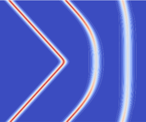
Figure 7(a–c) depicts a numerical simulation of the truncated soliton initial data (3.15) with  $\ell = 300$ that has been smoothed so as to minimise Gibbs type oscillations (Biondini & Trogdon Reference Biondini and Trogdon2017). Curved waves emanate from the truncation edges as the central portion propagates forward. When the central prominence decays, the entire wave forms a curved shape with decaying amplitude and curvature as time increases. These qualitative features are reflected in the obtained modulation solution for the soliton amplitude
  $a(y,t)$ and slope
  $q(y,t)$ in (3.4a,b), (3.12). In order to quantitatively compare the simulation to modulation theory predictions, we extract the modulated soliton amplitude and slope from the simulation via
 \begin{equation} a(y,t) = \max_{x \in \mathbb{R}} u(x,y,t), \quad q(y,t) = -\left( \textrm{arg max}_{x \in \mathbb{R}} u(x,y,t)\right)_y . \end{equation}
For the numerical computation of  $q$, we smooth
  $\rm{arg max} u$ prior to differentiation. Figure 7 bottom displays the numerical (solid) and modulation (dashed) solutions. In order to quantitatively track the numerical simulation, we used the slightly smaller truncation width
  $\ell = 280$ for the modulation solution in order to account for the smoothing of the initial data as given in (B 6a,b). Both the soliton amplitude and slope closely match the full partial differential equation (PDE) evolution described by (1.1), demonstrating that our modulation analysis captures both the qualitative and quantitative features of the solution. The long-time (
 $T \gg 1$) asymptotic predictions in (3.14) for a parabolic, decaying cKdV soliton also compare favourably with the numerical and modulation solutions for
  $|y| \lessapprox \ell$ despite the modest scaled time
  $T = t/\ell \approx 1.5$.

Figure 7. (a–c) Numerical evolution of truncated soliton initial data (B 6a,b) according to the KPII equation for  $t \in (0,150,500)$ and
  $\ell = 300$. (d,e) Modulated soliton amplitude
  $a$ and slope
  $q$ at noted times extracted from the numerical simulation (solid curves) and the modulation solution (3.4a,b), (3.12) (dashed curves) with the slightly different, fitted initial soliton length
  $\ell = 280$. The dash-dotted blue lines correspond to the long-time asymptotic predictions (3.14) evaluated at
  $t = 500$.
In summary, the truncated soliton initial data (3.15) evolve into a curved soliton with algebraically decaying amplitude that approaches a cKdV soliton with a parabolic profile and linearly increasing focal length.
4. Bent-stem and bent line solitons
The modulation solution for the truncated soliton consisting of two counterpropagating and then interacting simple waves motivates a broader class of initial conditions where we relax the assumption of zero soliton amplitude for  $|y| > \ell /2$. In this section, we explore this scenario with three distinct configurations: a special partially bent soliton, two bent solitons joined via a larger amplitude stem with non-zero
  $\ell$ and finally a bent soliton with the same amplitude throughout in which
  $\ell \to 0$ – the regular and Mach expansion problem. First, we consider the partially bent soliton as a natural extension of the partial line soliton described in § 3.1.
4.1. Partially bent solitons
We first consider a single bend at  $y = 0$ where
 \begin{equation} a(y,0)= \begin{cases} 1,
& y \leqslant 0, \\ a_0, & y > 0, \end{cases} \quad q(y,0)=
\begin{cases} 0, & y \leqslant 0, \\ q_0, & y > 0.
\end{cases}
\end{equation}
\begin{equation} a(y,0)= \begin{cases} 1,
& y \leqslant 0, \\ a_0, & y > 0, \end{cases} \quad q(y,0)=
\begin{cases} 0, & y \leqslant 0, \\ q_0, & y > 0.
\end{cases}
\end{equation}
For generic choices of  $0 < a_0 < 1$ and
  $0 < q_0 < 1$, the initial data (4.1a,b) give rise to two separated simple wave solutions of the modulation equations (1.4): a fast 2-RW and a slow 1-RW separated by a constant region. As a natural extension of the partial line soliton solution (3.2), we restrict the data (4.1a,b) so that only a single simple wave – the 1-RW – is generated, i.e.
  $s = q + \sqrt {a}$ is constant
 \begin{equation} q_0 + \sqrt{a_0} = 1, \quad 0 < a_0 < 1, \quad 0 < q_0 < 1 . \end{equation}
We call the corresponding initial data (4.1a,b) subject to (4.2a–c) a partially bent soliton, which will be useful to describe the bent-stem soliton initial data in the next subsection. The constancy of  $s$ (
$s$ ( $q(y,t) + \sqrt {a(y,t)} = 1$) and
  $U(a,q) = y/t$ result in the 1-RW solution
 \begin{equation} \left. \begin{gathered}
\sqrt{a_{pb}(y,t)} = \begin{cases} a_0, & U_0 t < y,
\\ \frac{3}{4} ( 1- {y}/({2t})), & -\frac{2}{3} t < y < U_0 t, \\
1, & y < -\frac{2}{3} t, \end{cases}\\ q_{pb}(y,t)
= 1 - \sqrt{a_{pb}(y,t)}, \quad U_0 = 2 -
\tfrac{8}{3}\sqrt{a_0} . \end{gathered}\right\}
\end{equation}
\begin{equation} \left. \begin{gathered}
\sqrt{a_{pb}(y,t)} = \begin{cases} a_0, & U_0 t < y,
\\ \frac{3}{4} ( 1- {y}/({2t})), & -\frac{2}{3} t < y < U_0 t, \\
1, & y < -\frac{2}{3} t, \end{cases}\\ q_{pb}(y,t)
= 1 - \sqrt{a_{pb}(y,t)}, \quad U_0 = 2 -
\tfrac{8}{3}\sqrt{a_0} . \end{gathered}\right\}
\end{equation}
This solution is the same as that of the partial soliton (3.2) for  $y < U_0 t$ and limits to the partial soliton modulation as the angled soliton amplitude vanishes
  $a_0 \to 0$. The positive amplitude, outgoing soliton gives rise to the slower characteristic velocity
  $U_0 < 2$. The evolution of a partially bent soliton (4.1a,b) with
  $\sqrt {a_0} = 0.7$,
  $q_0 = 0.3$ according to numerical integration of the KP equation (1.1) is shown in figure 8(a–c). The 1-RW modulation solution's edge characteristic velocities
  $U_0$ and
  $-\frac {2}{3}$ in (4.3) are favourably compared with the numerical simulation in figure 8(d,e) by identifying the front positions where
  $a \to 0.52$ and
  $a \to 0.97$, respectively.

Figure 8. (a–c) Numerical evolution of the partially bent soliton according to the KPII equation for  $t \in (0,150,400)$ and
  $\sqrt {a_0} = 0.7$,
  $q_0 = 0.3$. (d,e) Comparison of the characteristic speeds of the upper (d) and lower (e) edges of the partially bent soliton rarefaction wave. The plot displays the predicted front speeds from the modulation solution (4.3) as reference lines (dash-dotted, blue), the numerically extracted front positions from the numerical simulation (solid, black) and a least squares linear fit (dashed, red) whose slope determines the measured speeds.
The solution (4.3) provides a building block to analyse the more complicated configuration of a bent-stem soliton.
4.2. Bent-stem solitons
We now consider the initial condition
 \begin{equation} a(y,0)= \begin{cases} 1,
& |y| \leqslant \ell/2, \\ a_0, & |y| >
\ell/2, \end{cases} \quad q(y,0)= \begin{cases} 0, & |y|
\leqslant \ell/2, \\ \mathrm{sgn}(y) q_0,
& |y| >\ell/2, \end{cases}
\end{equation}
\begin{equation} a(y,0)= \begin{cases} 1,
& |y| \leqslant \ell/2, \\ a_0, & |y| >
\ell/2, \end{cases} \quad q(y,0)= \begin{cases} 0, & |y|
\leqslant \ell/2, \\ \mathrm{sgn}(y) q_0,
& |y| >\ell/2, \end{cases}
\end{equation}
which is the modulation initial condition for the KPII data depicted in figure 4(b). This configuration describes an initial truncated soliton of length  $\ell$ that is extended with outgoing line solitons of amplitude
  $a_0 < 1$ and non-zero, symmetric slopes
  ${\pm } q_0$. The case
  $a_0 = 0$ and
  $q_0 = 1$ corresponds to the truncated soliton (3.3). As similarly noted for the partially bent soliton, generic choices of
  $0< a_0 < 1$ and
  $0 < q_0 < 1$ will give rise to four separated non-centred simple waves, two emanating from each bend
  $y = \pm \ell /2$. The fastest and slowest waves, however, will not interact with the other waves, propagating far away from the initial stem region. These non-interacting, propagating waves are of less interest so we restrict the initial data such that a single simple wave is generated at each bend, as in the partially bent soliton case. Consequently, we assume the same simple wave constraint in (4.2a–c) corresponding to a non-centred 1-RW emanating from
  $y = \ell /2$ and a non-centred 2-RW emanating from
  $y = -\ell /2$. We call the corresponding initial data (4.4a,b) a bent-stem soliton.
This initial value problem is nearly identical to the truncated soliton problem. In fact, their solutions are essentially the same apart from one subtle yet crucial difference: the velocities of the outermost edges of the counterpropagating simple waves are different. These differing velocities lead to different interaction features.
We now use the partially bent soliton simple wave (4.3) to construct the counterpropagating simple waves for the bent-stem soliton initial data (4.4a,b)
 \begin{equation} a(y,t) = a_{pb}(|y|-\ell/2,t), \quad q(y,t) = \mathrm{sgn}(y)q_{pb}(|y|-\ell/2,t), \end{equation}
for  $y \in \mathbb {R}$ prior to simple wave interaction
  $0 \leqslant t \leqslant \frac {3}{4}\ell$.
Compared to the truncated soliton, the Riemann invariants for the bent-stem soliton simple waves take values on the smaller square
 \begin{equation} (r,s) \in [-1,r_0] \times [-r_0,1]\quad {\mathrm{where}}\ r_0 = 1-2\sqrt{a_0} < 1 . \end{equation}
Consequently, the hodograph solution for the simple wave interaction region is the same as for the truncated soliton, namely (3.9). However, the solution must be considered on the restricted domain (4.6). Two space–time characteristic diagrams of the modulation solution for different values of  $a_0$ are shown in figure 9. The interaction region is shaded grey. The bottom point of the interaction region corresponds to the initiation of simple wave interaction when
  $(Y,T) = (0,\frac {3}{4})$. Note that the characteristic for the uppermost edge of the incoming 1-RW,
  $Y = \frac {1}{2} + U_0 T$, eventually intersects the edge of the interaction region (3.11) at
  $(Y_*,T_*)$. Similarly, the reflected characteristic emanating from
  $Y = -\frac {1}{2}$ intersects the interaction region at
  $(-Y_*,T_*)$. These intersection points are given by
 \begin{equation} Y_* = \frac{1}{2} + \frac{3- 4\sqrt{a_0}}{2a_0} , \quad T_* = \frac{3}{4 a_0} \end{equation}
and are shown in the characteristic diagrams of figure 9 for two different choices of  $a_0$. When
  $a_0 \to 0$,
  $T_* \to \infty$ and we recover the result for the truncated soliton in which the colliding simple waves do not completely intersect one another. For the bent-stem soliton in which
  $0 < a_0 < 1$, the existence of the intersection points
  $({\pm } Y_*,T_*)$ occurs because the characteristic velocity
  $U_0$ is slower than the corresponding characteristic velocity of the truncated soliton
  $U_0 < 2$. This subtle velocity difference leads to a significant change in the dynamics as we now explain.

Figure 9. Characteristic plots of interacting simple waves for the bent-stem soliton initial data (4.4a,b); (a)  $0 < a_0 \leqslant \frac {1}{4}$, resulting in an infinite region of interaction for two simple waves in
  $(y,t)$-plane, (b)
  $\frac {1}{4} < a_0 < 1$, resulting in a bounded interaction region. See main text for description.
For  $T > T_*$, the 2-RW that propagated from the lower bend at
  $y = -\ell /2$ emerges from the interaction region as a simple wave with constant
  $r = r_0$ and expands along the upper, outgoing soliton. The uppermost, leading edge portion of the simple wave is the straight line characteristic
 \begin{equation} Y = V_0 (T - T_*) + Y_*, \quad V_0 = V(r_0,1) = \tfrac{2}{3}(2\sqrt{a_0}+1) . \end{equation}
The boundary of the interaction region emanating from  $(Y_*,T_*)$ now becomes the parametric curve
 \begin{equation} Y = Y(r_0,s), \quad T = T(r_0,s) , \quad s \in [-r_0,1] , \end{equation}
where  $Y_* = Y(r_0,1)$,
  $T_* = T(r_0,1)$ and the curve is traversed as
  $s$ is decreased from 1. A new Cauchy problem for the modulation equations (1.4) must be solved with data prescribed along the parametric curve (4.9). Because the region into which this Cauchy problem propagates is constant,
  $(a,q) = (a_0,q_0)$, it is a simple wave, a 2-wave with
  $r = r_0$. The solution is determined by identifying the characteristics emanating from the boundary curve (4.9). Given any
  $s \in (\max(-r_0,0),1)$ along the boundary curve (4.9), the corresponding characteristic along which
  $s$ is constant is the straight line
 \begin{equation} Y = \tfrac{2}{3}(r_0 + 2s)(T-T(r_0,s)) + Y(r_0,s) . \end{equation}
Example characteristics are shown in figure 9(b).
A bifurcation occurs in the shape of the interaction region depending on the initial outgoing soliton amplitude  $a_0$. For sufficiently large
  $a_0$, the interaction boundary (4.9) terminates when
  $Y = 0$, which from the hodograph solution (3.9b) occurs when
  $s = -r_0$. According to the parametric curve (4.9), it would appear that
  $s = -r_0$ can occur for any
  $-1 \leqslant r_0 < 1$. However, the hodograph solution for
  $T$ in (3.9a) shows that
  $T \to \infty$ as
  $s \to r_0$. As
  $s$ is decreased from
  $1$ in the parametric curve (4.9),
  $s$ attains the value
  $r_0$ before it reaches
  $-r_0$ if and only if
  $r_0 > 0$. Consequently, the critical value
  $r_0 = 0$ determines the bifurcation from an unbounded (when
  $0 \leqslant r_0 \leqslant 1$) to a bounded (when
  $-1 < r_0 < 0$) simple wave interaction region. We now consider each case in turn.
The characteristic diagram for an unbounded interaction case where  $r_0 > 0$ (equivalent to either condition
  $0 < a_0 \leqslant 1/4$ or
  $1/2 \leqslant q_0 < 1$) is shown in figure 9(a). Aside from the intersecting characteristics at
  $({\pm }Y_*,T_*)$ and the concomitant simple wave (4.10) that emerges from the interaction region, the bent-stem soliton diagram is similar to the truncated soliton solution in which
  $a_0 = 0$ (cf. figure 6). In fact, the long-time asymptotic behaviour of the solution is identical to the truncated line soliton (3.14) when
  $|Y| \leqslant T^{2/3}$ in which the stem forms a decaying soliton that approaches the parabolic-shaped cKdV soliton (3.20a,b).
In contrast, when  $r_0 < 0$ (equivalent to either
  $1/4 < a_0 < 1$ or
  $0 < q_0 < 1/2$), corresponding to the case of a bounded simple wave interaction region, the characteristic diagram is significantly different as in figure 9(b). By symmetry, the interaction boundary must close at
  $Y_{c} = 0$. Since
  $s = -r_0$ determines the terminus of interaction, the corresponding closing time
  $T_{c}$ can be calculated from the hodograph solution (3.9a)
 \begin{equation} T_{c} = -3 \frac{1+r_0^{2}}{8 r_0^{3}} = \frac{3(1-2\sqrt{a_0}+2 a_0)}{4(2\sqrt{a_0}-1)^{3}} . \end{equation}
The corresponding soliton slope is zero by reflection symmetry and the amplitude can be read off from  $s = -r_0$, giving
 \begin{equation} a(Y_{c},T_{c}) = a_{c} = (2\sqrt{a_0}-1)^{2}, \quad q(Y_{c},T_{c}) = q_{c} = 0 . \end{equation}
From this closing point, a constant region emerges, bounded by the edges of the simple wave (4.10) and its symmetric reflection
 \begin{equation} |Y| = V(r_0,-r_0)(T-T_{c}) = -\tfrac{2}{3} r_0 (T-T_{c}) = \tfrac{2}{3}(2\sqrt{a_0}-1)(T-T_{c}) . \end{equation}
This constant region corresponds to the emergence of a line soliton with amplitude  $0 < a_\textrm {c} < 1$. Our findings for the bent-stem soliton are summarised in table 1.
Table 1. Dynamics of the bent-stem soliton initial data (4.4a,b).

Figure 10 depicts the numerical evolution of bent-stem solitons for each of the scenarios in table 1. For figure 10(a–c), the initial conditions are nominally  $\sqrt {a_0}=0.8$ and
  $q_0=0.2$, with
  $\ell =100$. From our analysis, the emergence of a constant region in the modulation, i.e. a vertical soliton with amplitude
  $a_c = 0.36$, should begin to appear at
  $t = \ell T_c \approx 236$. By
  $t=400$ in figure 10(c), the vertical soliton has emerged with amplitude very close to the predicted value
  $0.36$ shown in figure 11(a). In contrast, for figure 10(d–f), the initial conditions are
  $\sqrt {a_0}=0.3$ and
  $q_0=0.7$, again with
  $\ell =100$. As expected, the system forms a parabola which slowly decays over time.

Figure 10. (a–c) Numerical simulation of the bent-stem soliton for  $\sqrt {a_0}=0.8$ and
  $q_0=0.2$ with
  $t \in (0,80,400)$ showing the emergence of a straight line soliton. The interaction region closing time is predicted to be
  $t = \ell T_{c} = 236$ (cf. figure 9b). (d–f) Numerical simulation of the bent-stem soliton for
  $\sqrt {a_0}=0.3$ and
  $q_0=0.7$ with
  $t \in (0,80,400)$ leading to a decaying parabolic soliton. In both cases,
  $\ell = 100$.

Figure 11. Comparison between numerical simulation (solid line) and the modulation solution (dashed line) of the bent-stem amplitude decay at  $y=0$ for the parameters in figures 10(a) and 10(f). In order to account for the smooth initial data, the modulation solution is ‘fitted’ by choosing
  $\ell =80$.
For quantitative analysis, we consider the amplitude decay at  $y=0$ for the bent-stem simulations in figure 11. In (a) is displayed the amplitude decay for the weakly bent simulation shown in figure 10(a–c), while in (b) are data from the strongly bent simulation from figure 10(d–f). Here, we observe some deviation of the numerical simulation from modulation theory for shorter times. We attribute these differences to higher order dispersive effects that are not captured by the leading-order modulation equations (1.4). However, the large
  $t$ predicted behaviour agrees quantitatively with numerical simulations. For the weakly bent stem, the amplitude asymptotically approaches
  $a_c=0.36$ as predicted, while for the strongly bent-stem case, the amplitude continues to decrease for large t. As in the truncated case, we slightly reduce the length
  $\ell$ in the modulation solution to
  $\ell =80$ in order to account for the smoothing of the initial conditions.
We also consider the predicted soliton phase  $\xi$ compared to the numerical simulations. This is shown in figure 12. The overlaid predicted phases (dashed curves) were generated by using the modulation solution for
  $q$ and then numerically integrating for
  $\xi$ according to (1.5). We utilised the speed
  $c(y,t)$ in the prediction after fitting the phase so that it lines up with the front's maximum along
  $y = 0$ at
  $t = 100$ in the left-most panels. The ensuing phase profiles at
  $t = 200$ and
  $t = 400$ are slightly advanced relative to the numerical simulation, which can be attributed to higher-order phase errors that are common in soliton perturbation theory. Such a correction would result in an additional term
  $\xi _0(x,y,t)$ being added to the modulated soliton phase
  $\xi$ in (1.5). Importantly, the shape of the front's crest is well-described by the modulation solution for
  $q$.
$q$.

Figure 12. Modulation solution phase (dashed) overlaid on contour plots for weakly (a–c) and strongly (d–f) bent-stem initial conditions when  $t \in (100,200,400)$. The initial conditions are the same as in figure 10.
It is evident that both the weakly and strongly bent-stem numerical evolutions are well approximated by the modulation solution, asymptoting to a line soliton and a parabolic wave in long time, respectively.
4.3. Bent solitons
We now consider the bent-stem soliton initial data (4.4a,b) with a vanishing stem  $\ell \to 0$, i.e. a bent soliton in which
 \begin{equation} a(y,0)=a_0, \quad
q(y,0)= \begin{cases} q_0, & y>0, \\ -q_0, & y \leqslant 0.
\end{cases} \end{equation}
\begin{equation} a(y,0)=a_0, \quad
q(y,0)= \begin{cases} q_0, & y>0, \\ -q_0, & y \leqslant 0.
\end{cases} \end{equation}
Figure 4(c) displays the corresponding initial condition for the KPII equation (1.1). In contrast to the truncated and bent-stem soliton initial conditions, the initial conditions (4.14) for the modulation equations (1.4) correspond to a Riemann problem. We limit our consideration to an expansive Riemann problem by taking  $q_0>0$. This case corresponds to a partial soliton interacting with an expansive corner (cf. figure 3). If
  $q_0 < 0$, a case we do not consider, the partial soliton interacts with a compressive corner and gives rise to regular and Mach reflection (cf. figure 2).
For the case where  $q_0 + \sqrt {a_0} = 1$, cf. (4.2a–c), the bent soliton's evolution can be obtained directly from the bent-stem soliton evolution by taking the vanishing stem limit
  $\ell \to 0$. Consequently, the bent soliton inherits the bent-stem soliton's bifurcation in the long-time dynamics. When
  $\sqrt {a_0} > q_0$, the modulation solution for the bent-stem soliton post-simple wave interaction (
 $T > T_{c}$) exhibits an expanding constant region with
  $a = a_{c}$,
  $q = q_{c}$ in (4.12a,b) bounded by the characteristics (4.13). We refer to this as the strong interaction case.
When  $\sqrt {a_0} < q_0$ and
  $q_0 + \sqrt {a_0} = 1$, we can take the
  $\ell \to 0$ limit of the bent-stem soliton with an unbounded interaction region. In this limit, the corners of the interaction region in (4.7a,b) are
  $(\pm y_*,t_*) = (\pm \ell Y_*,\ell T_*) \to (0,0)$. Additionally, the interaction boundaries (3.11) and (4.9) collapse to
  $y = 0$. However, the characteristics (4.10) leaving the boundaries of the interaction region persist. At
  $y = 0$, the soliton amplitude in the interaction region is explicitly (3.13a) so that
  $a(0,t) \to 0$ as
  $\ell \to 0$. This case corresponds to weak interaction.
In order to elucidate more details and provide an alternative method of solution, we now solve the Riemann problem (4.14) for the bent soliton directly. We relax the assumption  $q_0 + \sqrt {a_0} = 1$ and consider general
  $a_0 > 0$ and
  $q_0 > 0$, which is equivalent to applying the scaling symmetry (2.1a) to the bent-stem soliton problem and taking
  $\ell \to 0$.
First, we consider the strong interaction case  $\sqrt {a_0}>q_0$. The upper and lower solitons cannot be connected by a single simple wave, which would require
  $\sqrt {a_0}-q_0=\sqrt {a_0}+q_0$, leading to the conclusion
  $q_0 = 0$. Instead, we introduce the intermediate state
  $(a_\textrm {i},q_\textrm {i})$ and connect it to
  $(a_0,\pm q_0)$ with simple waves satisfying
 \begin{equation} \sqrt{a_{i}}-q_{i} = \sqrt{a_0}-q_0 , \quad \sqrt{a_{i}}+q_{i} = \sqrt{a_0}+(-q_0) . \end{equation}
The solution to these equations under the given constraints is
 \begin{equation} q_{i}=0, \quad \sqrt{a_{i}}=\sqrt{a_0}-q_0, \end{equation}
where we use a 2-RW to connect the intermediate state to the top soliton and a 1-RW to connect to the bottom soliton.
Consequently, evolving the bent soliton over time gives an intermediate constant region connected to the two canted solitons by centred simple waves
 \begin{equation} \left. \begin{gathered}
\sqrt{a(y,t)} = \begin{cases} \sqrt{a_0}, & V(a_0,q_0)t <
|y|, \\
\frac{3}{8}({y}/{t}+2\sqrt{a_{i}}), & V(a_{i},0)t < |y|
< V(a_0,q_0)t, \\ \sqrt{a_{i}}, & |y| <
V(a_{i},0)t, \end{cases}\\ q(y,t) =
\mathrm{sgn}(y) \begin{cases} q_0, & V(a_0,q_0)t < |y|,
\\ \sqrt{a(y,t)}-\sqrt{a_{i}}, &
V(a_{i},0)t < |y| < V(a_0,q_0)t, \\ 0, &
|y| < V(a_{i},0)t, \end{cases} \end{gathered}\right\}
\end{equation}
\begin{equation} \left. \begin{gathered}
\sqrt{a(y,t)} = \begin{cases} \sqrt{a_0}, & V(a_0,q_0)t <
|y|, \\
\frac{3}{8}({y}/{t}+2\sqrt{a_{i}}), & V(a_{i},0)t < |y|
< V(a_0,q_0)t, \\ \sqrt{a_{i}}, & |y| <
V(a_{i},0)t, \end{cases}\\ q(y,t) =
\mathrm{sgn}(y) \begin{cases} q_0, & V(a_0,q_0)t < |y|,
\\ \sqrt{a(y,t)}-\sqrt{a_{i}}, &
V(a_{i},0)t < |y| < V(a_0,q_0)t, \\ 0, &
|y| < V(a_{i},0)t, \end{cases} \end{gathered}\right\}
\end{equation}
where  $V(a,q) = 2q + \frac {2}{3} \sqrt {a}$. The solution contains a vertical line soliton expanding in
  $y$ with amplitude
  $a_\textrm {i}$ in (4.16a,b). A space-time contour plot of the amplitude a(y,t) for this case is shown in figure 13(a). This solution agrees with our analysis of the
  $\ell \to 0$ limit of the bent-stem soliton when
  $q_0 + \sqrt {a_0} = 1$. As we will show in the next subsection, this strong interaction case corresponds to Mach expansion of a soliton interacting with a corner.

Figure 13. Space–time contour plots of amplitude modulation solutions for bent soliton initial data. (a) The strong interaction case (4.15a,b) with  $a_0 = 1 > q_0 = 0.3$. (b) The weak interaction case (4.20) with
  $a_0 = 1 < q_0 = 1.4$. The two cases are similar but note the non-zero central amplitude for strong interaction.
For weak interaction when  $\sqrt {a_0} < q_0$, the above calculation fails because
  $\sqrt {a_{i}}$ exhibits negative values. This determines the critical slope
 \begin{equation} q_{cr} = \sqrt{a_0} \end{equation}
between the two classes of bent soliton dynamics. Instead, we introduce the intermediate vacuum state  $a_{i} = 0$. In order to connect to vacuum with a simple wave from each of the bent solitons, we require
  $q_{i} \ne 0$. Since
  $q$ in the vacuum region is undefined, we determine it locally based on the simple wave criterion. By symmetry,
 \begin{equation} q_{i+} = \lim_{y \to 0^{+}} q(y,t)=-\lim_{y \to 0^{-}}q(y,t) =q_{i-}, \end{equation}
with the initial discontinuity at  $y=0$. We can use Riemann invariants to calculate the values of
  $q_{i \pm }$. For the top simple wave,
  $\sqrt {a_0}-q_0=-q_{i +}$, and by symmetry
  $q_{i +}=-q_{i -}$. The solution for the simple wave is
 \begin{equation} \left. \begin{gathered}
\sqrt{a(y,t)} = \begin{cases} \sqrt{a_0}, & V(a_0,q_0)t <
|y|, \\ \frac{3}{8}({y}/{t}-2q_{i +}),
& V(0,q_{i +})t < |y| < V(a_0,q_0)t, \\ 0,
& |y| < V(0,q_{i +})t, \end{cases}\\ q(y,t) =
\mathrm{sgn}(y) \begin{cases} q_0, & V(a_0,q_0)t < |y|,
\\ \sqrt{a(y,t)}+q_{i +}, & V(0,q_{i +})t
< |y| < V(a_0,q_0)t, \\ q_{i +}, & |y| <
V(0,q_{i +})t, \end{cases} \end{gathered}\right\}
\end{equation}
\begin{equation} \left. \begin{gathered}
\sqrt{a(y,t)} = \begin{cases} \sqrt{a_0}, & V(a_0,q_0)t <
|y|, \\ \frac{3}{8}({y}/{t}-2q_{i +}),
& V(0,q_{i +})t < |y| < V(a_0,q_0)t, \\ 0,
& |y| < V(0,q_{i +})t, \end{cases}\\ q(y,t) =
\mathrm{sgn}(y) \begin{cases} q_0, & V(a_0,q_0)t < |y|,
\\ \sqrt{a(y,t)}+q_{i +}, & V(0,q_{i +})t
< |y| < V(a_0,q_0)t, \\ q_{i +}, & |y| <
V(0,q_{i +})t, \end{cases} \end{gathered}\right\}
\end{equation}
which includes a symmetric reflection for the bottom simple wave. This solution, whose amplitude a(y,t) is depicted in a contour plot in figure 13(b), consists of an expanding vacuum  $a = 0$ region connected to outgoing, canted line solitons by simple waves. These simple waves are rotated versions (see (2.1b)) of the partial soliton solution (3.2). They are completely disconnected from one another; at this order of approximation, the interaction is negligible in that the evolution of the upper and lower branches can be analysed independently of one another. The vacuum region's rate of expansion is proportional to
  $q_0-\sqrt {a_0} > 0$. A more ‘bent’ initial soliton (
 $q_0 > q_\textrm {cr}$) causes the outgoing solitons to separate from one another sufficiently fast so that their interaction is negligible within the context of modulation theory. As we will show in the next subsection, this weak interaction case corresponds to regular expansion of a soliton interacting with a corner.
The numerical simulations in figure 14 are essentially consistent with these predictions. For the bent soliton with  $a_0=1$ and
  $q_0=1.4 > q_{cr} = 1$ in figure 14(d–f), a decaying parabolic front with trailing oscillations appears. Although an expanding, strictly vacuum region predicted by modulation theory is not immediately apparent, amplitude decay is present. We have verified that the amplitude, shape, and propagation of the leading parabolic front is consistent with the profile for the cKdV parabolic soliton (3.20a,b). The trailing oscillations are consistent with a two-dimensional generalisation of the oscillatory shelf that is common for perturbed KdV (cKdV) problems. In contrast, for an initial bent soliton with
  $a_0=1$ and
  $q_0=0.3 < q_{cr} = 1$, as seen in figure 14(a–c), a new vertical line soliton with reduced amplitude appears.

Figure 14. Numerical simulation of bent solitons for the strong interaction when  $a_0=1$,
  $q_0=0.3$ for
  $t \in (0,150,400)$ in (a–c) and the weak interaction when
  $a_0=1$,
  $q_0=1.4$ when
  $t \in (0,60,220)$ in (d–f).
Quantitative results further confirm our analysis. In figure 15, it is evident that the predicted solution for both soliton amplitude and slope, extracted according to (3.25a,b) captures the behaviour of the strong interaction case with  $a_0=1$ and
  $q_0=0.3 < q_{cr} = 1$. As expected, the solution for large times approaches a line soliton with
  $a_{i} \approx 0.49$.


For the weak interaction case  $q_0 = 1.4 > q_{cr} = 1$ shown in figure 16 (
 $\ell = 0$ case), the simulation's lead wave slope (solid) is well approximated by the modulation solution (dash-dotted). The amplitude does not reach zero as modulation theory predicts, although it does continually decrease. Recalling that modulation theory applies under slowly varying assumptions, it is not surprising that an immediate transition from unit amplitude to zero amplitude does not occur in the numerical simulation. In figures 11 and 15, we observe that the numerical solution temporally lags behind the modulation solution. The same happens here in figure 16, albeit to a more significant degree in amplitude. While this weakly interacting bent soliton simulation deviates from the modulation solution in amplitude, in fact it can be reasonably approximated by the bent-stem modulation solution for moderate stem length
  $\ell$. This is to be expected; the bent-stem analysis for sufficiently large
  $q_0$ shows that any positive stem length
  $\ell >0$ implies algebraic amplitude decay to zero (cf. (3.14)) rather than a sudden amplitude decrease to zero in finite time. The initial smoothing of the numerical simulations (see appendix B) can be viewed as an effective
  $\ell >0$ for these bent soliton simulations. Consequently, we compare the bent-stem soliton modulation solution for the initial data (4.4a,b) (rescaled according to (2.1a) so that the canted, outgoing solitons have unit amplitude) with
  $\ell = 12$ to the numerical simulation of the weakly interacting bent soliton in figure 16. Now the decaying parabolic front is represented in the modulation solution. In other words, the weakly interacting bent soliton evolution exhibits a remnant of the bent-stem soliton solution.

Figure 16. Comparison of bent-stem soliton modulation with small stem  $\ell = 12$ (dashed, red) and no stem
  $\ell \to 0$ (dash-dotted, blue) to numerical simulation (solid, black) of the weakly interacting bent soliton evolution in figure 14(d–f).
4.4. Regular and Mach expansions
We are now in a position to interpret this analysis in the context of the soliton-corner initial-boundary value problem that is schematically depicted in figure 3. Consider a vertical, partial soliton with amplitude  $a$ propagating in the positive
  $x$ direction adjacent to a horizontal wall located at
  $y = 0$. When this soliton encounters a corner at the origin that suddenly opens or turns away by the clockwise angle
  $\varphi > 0$, it expands. The nature of its expansion depends on the corner angle and soliton amplitude. Via the nonlinear method of images, we map the partial soliton at the moment it encounters the corner to the bent soliton initial data for the numerical simulation in figure 4(c) and for modulation theory in (4.14) with
  $a_0 = a$ and
  $q_0 = \tan {\varphi }$. Consequently, the critical corner angle separating two distinct types of soliton-corner interaction is (cf. (4.18))
 \begin{equation} \tan{\varphi_{cr}} = \sqrt{a}. \end{equation}
 For the case  $\varphi > \varphi _{cr} = \arctan {\sqrt {a}}$ (sharp corner), the soliton almost completely separates from the wall. The residual soliton–wall interaction is through a decaying parabolic soliton. In turn, the propagating partial line soliton decays, retreating further away from the wall. We term this case regular expansion. In contrast, for slight turns of the wall at the corner where
  $0 < \varphi < \varphi _{cr} = \arctan {\sqrt {a}}$, the soliton also develops a curved front that instead terminates at a non-decaying soliton perpendicular to the wall with lower amplitude than the incident soliton. The predicted soliton wall amplitude is
 \begin{equation} a_{w} = (\sqrt{a}-\tan{\varphi})^{2}. \end{equation}
Despite propagating away from the wall, it does not ‘escape’ its influence like in the regular expansion case. The residual soliton formed at the wall is the expansion counterpart to the Mach stem that forms during the course of Mach reflection (cf. figure 2). We term this case Mach expansion. Surprisingly, the cross-over from regular to Mach expansion occurs at precisely the same corner angle (4.21) as the crossover from regular to Mach reflection (1.3). These results are highlighted in table 2.
Table 2. Soliton-expansive corner initial-boundary value problem.

5. Discussion and conclusion
Using the KPII equation as a model of multidimensional gravity wave solitons, we describe the evolution of truncated and interacting oblique solitons using modulation theory and we compare the analytical predictions with the results from direct numerical simulations. The initial value problems considered are distinguished by geometric configurations of partial solitons that propagate away from one another. Despite this, residual interactions between solitons occur that lead to non-trivial wave patterns.
An initial soliton that is transversely confined or truncated, and that propagates into an open region, first ‘curls’ at the endpoints as it then morphs into a parabolic shape over long times. The front's parabolic shape flattens with a linearly increasing focal length with time. The parabolic wave's amplitude and speed exhibits algebraic decay proportional to  $t^{-2/3}$. Such wave patterns appear to be common in images of oceanic internal waves for near-shore conditions (Jackson Reference Jackson2004; Nash & Moum Reference Nash and Moum2005; Wang & Pawlowicz Reference Wang and Pawlowicz2017). In particular, figure 17 depicts internal solitary waves that strikingly resemble both the early and long time evolution of the truncated soliton solution considered here. A nearly straight solitary wave with curling edges and multiple parabolically shaped solitary waves are visible.

Figure 17. Synthetic aperture radar image of internal solitary waves generated at the Columbia River plume front. Reproduced with permission from Pan et al. (Reference Pan, Jay and Orton2007) copyright 2007 by the American Geophysical Union.
We also generalise the above truncated soliton configuration by appending canted partial solitons to it and find new dynamical behaviour. In addition to the decaying parabolic wavefront for sufficiently canted solitons, a non-decaying vertical soliton with reduced amplitude relative to the original soliton segment appears. This bifurcation in behaviour carries over to the soliton-corner expansion problem.
The final initial value problem for a bent soliton also describes the interaction of a soliton propagating parallel to a wall with an expansive corner. For a sharp enough bend, the solitons exhibit weak interaction through a decaying parabolic front, the case we identify as regular expansion of a soliton. For a slight enough bend, the solitons continue to interact so as to produce an intermediate, non-decaying soliton at the wall with reduced amplitude  $a_{w}$ (4.22) that connects them. This case of Mach expansion parallels the well-known Mach reflection of oblique solitons, both of which occur at the same critical angle and display a similar transition between strong and weak interactions. Such a transition in the wave dynamics could potentially be observed in the shallow water context by soliton generation from a moving disturbance (Lee & Grimshaw Reference Lee and Grimshaw1990; Li & Sclavounos Reference Li and Sclavounos2002) or by experiments analogous to previous shallow water studies involving Mach reflection (Perroud Reference Perroud1957; Melville Reference Melville1980; Li et al. Reference Li, Yeh and Kodama2011; Kodama & Yeh Reference Kodama and Yeh2016).
In the Mach reflection case, an important quantitative test of the theory is its prediction of amplitude amplification of the Mach stem at the wall. After properly taking into account a higher-order asymptotic approximation to shallow water waves than the KP equation, the soliton wall amplitude has been demonstrated to satisfactorily predict experiments across a range of incident soliton parameters (angle and amplitude) (Kodama & Yeh Reference Kodama and Yeh2016). This points to a possible quantitative test of the Mach expansion theory presented here by measuring the wall reduction factor
 \begin{equation} \alpha \equiv \frac{a_{w}}{a} = \left ( 1 - \frac{\tan{\varphi}}{\sqrt{a}} \right )^{2}, \quad \tan{\varphi} < \sqrt{a} \end{equation}
in similar shallow water experiments. The factor  $\alpha < 1$ is the ratio of wall soliton amplitudes post (
 $a_{w}$) and pre (
 $a$) corner interaction, respectively, predicted by KP theory. We note that, in order to achieve quantitative agreement with experiment, it may be necessary to incorporate higher-order effects such as those considered in (Kodama & Yeh Reference Kodama and Yeh2016).
These results also motivate the conjecture that outgoing gravity line solitons propagating away from one another with slopes  ${\pm }q_\infty$ and similar amplitudes
  $a_\infty$ lead to a decaying parabolic or negligible interaction region when sufficiently sloped
  $q_\infty \geqslant \sqrt {a_\infty }$ but leave a residual line soliton between them when
  $q_\infty < \sqrt {a_\infty }$.
This work demonstrates the practical utility and efficacy of soliton modulation theory to describe the rich nonlinear wave dynamics. All the solutions that we consider are globally existing simple wave or interacting simple wave solutions of the hyperbolic modulation equations. These solutions, when projected back onto a line soliton, quantitatively agree with direct numerical simulations of the KPII equation. Although not previously recognised as such, simple wave-modulated solitons can also be seen in a variety of previous KPII numerical studies (Funakoshi Reference Funakoshi1980; Kodama et al. Reference Kodama, Oikawa and Tsuji2009; Kao & Kodama Reference Kao and Kodama2012; Chakravarty et al. Reference Chakravarty, McDowell and Osborne2017). In particular, the transient portion of the reflected wave that develops during both regular and Mach reflection of a soliton by a corner appears to show a similar wave pattern to the partial soliton studied here. An intriguing problem is to consider the modulation equations with initial data that are compressive, i.e. that would give rise to shock solutions. Indeed, two colliding partial solitons and ‘V-shaped’ initial conditions (Kodama et al. Reference Kodama, Oikawa and Tsuji2009; Chakravarty et al. Reference Chakravarty, McDowell and Osborne2017) for regular and Mach reflection, give rise to compressive Riemann problems for the modulation equations (1.4). How are such initial value problems regularised? What do shocks mean in this modulation context?
Acknowledgements
The work of M.A.H. and S.R. was supported by NSF grant DMS-1816934. The work of M.M. was supported by the NSF GRFP. The work of G.B. was supported by NSF grant DMS-2009487. Authors thank the Fields Institute Focus Program on Nonlinear Dispersive Partial Differential Equations and Inverse Scattering in the summer of 2017 where this research was initiated.
Declaration of interests
The authors report no conflict of interest.
Appendix A. Derivation of the soliton modulation equations
Here we show how (1.4) can be directly derived from the KP equation (1.1) using multiple scales, without employing the full Whitham modulation theory. First, we introduce the rescaling
 \begin{equation} X = \epsilon x, \quad Y = \epsilon y, \quad T = \epsilon t \end{equation}
into the KPII equation (1.1)
 \begin{equation} \left(u_T + uu_X + \epsilon^{2} u_{XXX}\right)_X +u_{YY} = 0. \end{equation}
In order to study modulated line solitons, the asymptotic expansion
 \begin{align} \left. \begin{gathered} u(X,Y,T;\epsilon) = u_0(\xi,Y,T) + \epsilon u_1(\xi,Y,T) + \cdots, \quad u_0(\xi,Y,T) = a(Y,T) \,\mathrm{sech}^{2} \left ( \eta \xi \right ), \\ \eta \xi_X = \frac{1}{\epsilon} \sqrt{\frac{a(Y,T)}{12}}, \quad \eta \xi_Y = \frac{1}{\epsilon} \sqrt{\frac{a(Y,T)}{12}} q, \quad \eta \xi_T = -\frac{1}{\epsilon}\sqrt{\frac{a(Y,T)}{12}} c(a,q) , \end{gathered}\right\} \end{align}
is assumed where  $\xi$ is the fast variable. The coefficient
  $\eta (Y,T) = \sqrt {a(Y,T)/12}$ is determined by the consistency condition
  $\xi _{XY} = \xi _{YX} = 0$. The consistency condition
  $\xi _{YT} = \xi _{TY}$ yields the slope modulation equation (1.4b). The amplitude modulation equation (1.4a) is obtained by inserting the ansatz (A 3) into the KPII equation (A 2). At first order in
  $\epsilon$, we obtain an inhomogeneous ordinary differential equation for
  $u_1$ that, when integrated once with respect to
  $\xi$, is
 \begin{equation} -c \partial_{\xi} u_1 + \partial_{\xi} \left ( u_0 u_1 \right ) + \partial_{\xi\xi\xi} u_1 + q^{2} \partial_{\xi} u_1 = - \left ( \partial_T u_0 + 2 q \partial_Y u_0 + q_Y u_0 \right ) . \end{equation}
Solvability over the space of  $L^{2}(\mathbb {R})$ solutions is enforced by the orthogonality condition
 \begin{equation} \left ( \partial_T + 2 q \partial_Y + q_Y \right ) \int_{\mathbb{R}} u_0^{2} \, \mathrm{d}\xi = \left ( \partial_T + 2 q \partial_Y + q_Y \right ) \left (\frac{8\sqrt{3}}{3} a^{3/2}\right ) = 0, \end{equation}
which, upon simplification, results in the amplitude modulation equation (1.4a).
Appendix B. Numerical integration of the KP equation
To validate our analytical results, we implement the pseudospectral method described in Kao & Kodama (Reference Kao and Kodama2012), which utilises a hyper-Gaussian windowing function and Fourier discretisation for non-periodic data in  $y$ and periodic data in
  $x$. We essentially follow Kao & Kodama (Reference Kao and Kodama2012) with a few modifications. The method proceeds as follows. Instead of solving the KP equation (1.1) for the original function
  $u$, we instead solve an equivalent PDE for a windowed function
 \begin{equation} v(x,y,t) = W(y)u(x,y,t), \end{equation}
where
 \begin{equation} W(y) = \exp({-a_n |y/L_y|^{n}}), \end{equation}
with  $n = 27$ and
  $a_n = 1.111^{n}\ln {10}$. The rapid decay of
  $W(y)$ for
  $|y|$ near
  $L_y$ ensures that
  $v=0$ near the top and bottom boundaries of the domain so that its periodic extension is smooth. In this region, we assume that the solution
  $u$ asymptotes to non-modulated line solitons. Thus,
  $u$ can be decomposed as
 \begin{equation} u = v+(1-W)\hat{u}, \end{equation}
where  $\hat {u}$ are line solitons with constant
  $a$ and
  $q$ of the form shown in (1.2a,b). Inserting the transformation (B 3) into the KP equation (1.1), we obtain an equivalent PDE for the windowed function
  $v$
$v$
 \begin{equation} (v_t+vv_x+v_{xxx})_x +v_{yy} = (1-W)(W\hat{u}\hat{u}_x-(v\hat{u})_x+2W'\hat{u}_y+W''\hat{u})_x, \end{equation}
subject to the initial conditions
 \begin{equation} v(x,y,0) = u(x,y,0)-(1-W(y))\hat{u}(x,y,0). \end{equation}
The above PDE (B 4) is solved numerically. At each time  $t$ we reconstruct the true solution
  $u$ using (B 3). The advantage of this method is that since
  $v$ is zero at the domain boundaries, we obtain spectral convergence using a Fourier discretisation in space. In order to preserve spectral accuracy, the derivatives
  $\hat {u}_x$,
  $\hat {u}_y$,
  $W'$, and
  $W''$ on the right-hand side of (B 4a) are calculated analytically; this is one difference from Kao & Kodama (Reference Kao and Kodama2012) where these derivatives are calculated using finite difference approximations. Time stepping is performed with an integrating factor and the classic fourth-order Runge–Kutta scheme. Simulations are terminated before the windowing region is corrupted by non-solitonic data.
The numerical scheme described above is validated using an exact Y-shaped solution, also known as the Miles resonant soliton (see figure 18a and, e.g. Biondini & Kodama (Reference Biondini and Kodama2003) for the explicit form of the solution). By refining the time and space steps, convergence is obtained at  $t=10$ to approximately
  $10^{-12}$ in the 2-norm relative difference of the numerical and exact travelling wave solutions, as shown in figure 18(b,c). The rate of spatial convergence in figure 18(b) demonstrates that spectral accuracy is obtained. In order to ensure reasonable computation time and memory demands, the simulation parameters are fixed at the grid spacing
  ${\rm \Delta} x = 1/2$ and time step
  ${\rm \Delta} t = 10^{-3}$. Based on figure 18(b,c), this ensures 2-norm errors below
  $10^{-6}$ for resolving the
  $Y$-soliton solution up to
  $t = 100$. Simulations are run on domains of various sizes that depend upon the problem, typically with an area comparable to
  $[-512,512]^{2}$. To take full advantage of our system's graphics processing unit, we used single precision for all calculations presented in the main text.

Figure 18. Convergence of Y-shaped soliton (a) in space (b) and time (c). These simulations were run on the domain  $[-128,128] \times [-64,64]$ with
  ${\rm \Delta} x = {\rm \Delta} y$. For (b) we fixed
  ${\rm \Delta} t = 10^{-3}$, and for (c) we fixed
  ${\rm \Delta} x = {\rm \Delta} y = 1/4$.
One unique feature of our numerical simulations is the incorporation of the KP equation constraint requiring  $\int u_{yy} \,{\textrm {d} x} = 0$ (see Ablowitz & Villarroel Reference Ablowitz and Villarroel1991; Klein, Sparber & Markowich Reference Klein, Sparber and Markowich2007). The bent soliton initial conditions satisfy this constraint. For the initial conditions which do not satisfy the constraint, a reflection is added that ensures that
  $\int u_y \,{\textrm {d} x} = 0$, thereby satisfying the constraint. The reflected solitons have parameters
  $(a_r,q_r)$ defined by
 \begin{equation} a_r(y) = (1-\sqrt{a(y,0)})^{2}, \quad q_r = 0. \end{equation}
The full initial conditions including the reflection for the truncated and bent-stem cases are displayed in figure 19. Simulations are terminated before the reflected solitons influence the solution in the region of interest. We find that this approach to satisfying the non-local constraint is more efficient than an odd extension of the initial data, which would result in the generation and propagation of fast dispersive wavetrains that quickly corrupt the solution.

Figure 19. Full initial conditions for simulation of truncated (a) and bent-stem solitons (b), satisfying the constraint  $\int u_{yy}\,\mathrm {d} x = 0$.
To reduce the Gibbs phenomenon, initial data for the simulations are obtained by smoothing the discontinuous initial data  $a(y,0)$ and
  $q(y,0)$ and inserting these data into (1.5). For example, the truncated soliton data (3.3) become
 \begin{equation} u(x,y,0) = a(y,0) \,\mathrm{sech}^{2}\left ( \sqrt{\frac{a(y,0)}{12}} x \right ), \quad a(y,0) = \frac{1}{2} \left ( \mathrm{tanh}\left ( \frac{\ell/2 - |y|}{w} \right ) + 1 \right ) , \end{equation}
with  $w = 5$,
  $\ell = 300$.
The two parameters of interest in this paper are the soliton amplitude and the soliton centre. The amplitude is obtained from the numerical results by finding the maximum value over  $x \in [-L_x,L_x]$ for each fixed
  $y$ and
  $t$ in the domain via local interpolation of the solution. The soliton centre is simply the location of that maximum value. These are then compared to the predicted amplitude and centre values. The predicted soliton centre is calculated using the analytical solution for
  $q(y,t)$ combined with (1.5) or, if
  $y$ is in the simple wave interaction region, using (3.17a,b). The numerical values for
  $q(y,t)$ are found by negating the numerically differentiated soliton centre location in
  $x$ with respect to
  $y$.
$y$.


