


1. Introduction
During the past century, mortality rates have been decreasing steadily all around the world. Even though some countries have experienced stagnations in mortality improvements during some periods (e.g. USA, England, and Denmark, see Ho and Hendi, Reference Ho and Hendi2018; Hiam et al., Reference Hiam, Harrison, McKee and Dorling2018; Aburto et al., Reference Aburto, Wensink, van Raalte and Lindahl-Jacobsen2018), the general consequence has been increases in life expectancies (but at different paces). Of course this is good news in terms of social progress; however, it also creates huge financial challenges for governments, life insurance companies, private pension funds, and individuals. Therefore, it is crucial to be able to understand and project mortality trends. For this purpose, demographers, statisticians, and actuaries have developed numerous mortality models in order to find appropriate methods for fitting and forecasting mortality and life expectancy.
Stochastic mortality models have become the standard approach for modeling and forecasting mortality. The pioneering contribution was the Lee and Carter (Reference Lee and Carter1992) model, and ever since their contribution, a wide range of extensions and variants have been developed. Stochastic mortality models typically decompose mortality rates into three dimensions (or any combination of the three): age, period, and cohort. After fitting the model, the time and cohort components are forecast using standard Box–Jenkins (ARIMA) procedures. To overcome the identifiability issues related to the estimation of stochastic mortality models, some studies suggest estimating the models as state space models (see, for example, Fung et al., Reference Fung, Peters and Shevchenko2017, Reference Fung, Peters and Shevchenko2019). Another issue of stochastic mortality models is related to their inability to model the age pattern of mortality decline in developed countries which is decelerating at younger ages and accelerating at older ages. This phenomenon is documented by Li et al. (Reference Li, Lee and Gerland2013) and called “rotation”. Li et al. (Reference Li, Lee and Gerland2013) propose an extended Lee–Carter (LC) method that accounts for this rotation. Another extension by Oeppen (Reference Oeppen2008) aims at improving mortality forecasts by forecasting the life table distribution of deaths using compositional data analysis (CoDA) for a LC type of model. CoDA models are particularly suitable for forecasting cause-specific deaths, since these models accurately account for the interdependence between causes of death.
While stochastic mortality models have gained ground within the mortality literature, data-driven machine learning methods from computer science and applied statistics have received a lot of attention in many other fields. This development has primarily been driven by the huge advances in computational power. Despite the many advantages of machine learning (such as flexibility, avoiding to impose structural assumptions, and good performance in- and out-of-sample), many researchers within the mortality literature are still reluctant to use the methods. This is primarily due to machine learning algorithms being viewed as “black boxes,” that is, that the internal workings of the algorithms are unclear to the researcher. As a consequence, the general perception is that machine learning results “lack interpretability.” Another drawback of machine learning methods is the potential risk of overfitting if not applied carefully.
Recent studies within the mortality literature have shown that machine learning has a huge potential in the context of modeling and forecasting mortality. These studies include, for example, tree-based techniques (see, for example, Deprez et al., Reference Deprez, Shevchenko and Wüthrich2017; Levantesi and Pizzorusso, Reference Levantesi and Pizzorusso2019 and Levantesi and Nigri, Reference Levantesi and Nigri2020) and neural network-based techniques (see, for example, Hainaut, Reference Hainaut2018; Richman and Wuthrich, Reference Richman and Wüthrich2019; Nigri et al., Reference Nigri, Levantesi, Marino, Scognamiglio and Perla2019, Reference Nigri, Levantesi and Marino2021, and Schnurch and Korn, Reference Schnürch and Korn2021). In most of the papers, the idea is to build on existing mortality models by adding a machine learning layer, thereby improving the fit and forecasts produced by these models. In particular, Deprez et al. (Reference Deprez, Shevchenko and Wüthrich2017) back-test the LC and the Renshaw and Haberman (Reference Renshaw and Haberman2006) models by applying one step of the Poisson regression tree boosting machine to calibrate a parameter, which is used to construct improved mortality rates. Following the same idea, Levantesi and Pizzorusso (Reference Levantesi and Pizzorusso2019) show that the model fit and forecast of the LC model can be improved by using either regression trees, random forests, or gradient boosting. Levantesi and Nigri (Reference Levantesi and Nigri2020) extend this work by combining random forests and two-dimensional P-splines to improve the fit and forecast of the LC model and show how this improved model affects the pricing of q-forward contracts. Additionally, they perform a “sensitivity to predictor” analysis in order to show in which demographic dimensions random forests improves the LC fit.
The work in Nigri et al. (Reference Nigri, Levantesi, Marino, Scognamiglio and Perla2019) proposes an alternative to the Box–Jenkins ARIMA approach for forecasting the time component in the LC model. In particular, they suggest a deep learning integrated LC model based on a recurrent neural network with long short-term memory architecture to forecast the time component. Schnurch and Korn (Reference Schnürch and Korn2021) propose to use a convolutional neural network to model and forecast mortality and implement a bootstrapping-based technique for quantifying the uncertainty of neural network predictions. Levantesi et al. (Reference Levantesi, Nigri and Piscopo2020) give an overview of the main results of the recent literature on machine learning and its applications for mortality predictions and longevity management.
In this paper, we investigate the ability of two tree-based machine learning models: random forests and gradient boosting, to make more accurate mortality forecasts and illustrate their potential for understanding past mortality trends and patterns. The advantages of tree-based techniques compared to neural networks are that they are less computationally expensive and relatively easy to understand and apply, partly because the training process is simpler, and partly because trees can be made “interpretable.” The latter is probably the most important advantage of tree-based techniques, since “interpretability” is often considered more important than forecasting performance.
The analysis in this paper is based on a pure random forests and a pure gradient boosting model in which we fit and forecast the differenced log-mortality rates. We compare mortality forecasts of a large set of models consisting of the pure random forests and gradient boosting models, ARIMA models combined with random forests and gradient boosting, nine different stochastic mortality models, and each of these nine models combined with random forests and gradient boosting. The combined models are based on the residuals from the stochastic models. In theory, these model residuals should reflect no more than random noise, and in that case random forests or gradient boosting should not be able to improve the performance of the stochastic models. If, however, the stochastic models were unable to detect certain patterns in the data, information is left in the residuals which can be detected by random forests or gradient boosting and used to improve the forecast. The forecast performances of the models are evaluated by applying the Model Confidence Set (MCS) procedure proposed by Hansen et al. (Reference Hansen, Lunde and Nason2011). The forecasting comparison shows that in the majority of cases considered, the pure random forests model and the pure gradient boosting model significantly outperform all the stochastic mortality models and their machine learning variants. A head-to-head comparison of each stochastic mortality model and its random forests and gradient boosting variants reveals that the tree-based methods do not always improve the forecasts of traditional models.
We further contribute to the literature by demonstrating how to “open up the black box.” That is, we show how to extract information from the random forests fit and show how this information can be used to better understand demographic dynamics. In particular, we propose to consider the variable split decisions made by the algorithms in order to detect the most frequent variable split points. Additionally, we consider variable importance and partial dependence plots which are typically provided or easily accessed through many of the available random forests and gradient boosting programs. Since random forests and gradient boosting can be interpreted similarly, we only illustrate this for the random forests model (gradient boosting results are presented in the Appendix). The in-sample results suggest that tree-based methods can be a powerful tool for detecting patterns within and between variables that are not commonly identifiable with traditional methods.
The paper is organized as follows: Section 2 briefly describes the data. Section 3 presents the models used for constructing mortality forecasts with a focus on the random forests and gradient boosting models, and how they are implemented using various transformations. Section 4 describes how forecast performances are evaluated and compared using the MCS procedure. Section 5 presents and discusses the forecasting results, and Section 6 illustrates how to interpret the in-sample random forests results. Finally, Section 7 concludes.
2. Data
The data contain annual country and gender-specific mortality rates from the Human Mortality Database (HMD). Data are divided into training sets (fitting periods) and test sets (in-sample forecast periods). We consider 6 different combinations of fitting periods and forecast horizons (training and test sets) by varying the length of each. The lengths of the fitting periods considered are 26 and 51 years. Forecasts all end in 2016, and the horizons vary between 16 and 30 years. Table 1 gives an overview of the different training and test sets used in the analysis. Note that the fitting period 1936–1986 includes years prior to and during World War II. Of course, there are issues related to fitting periods that include structural breaks (such as changes in sanitary conditions, advances in medicine, a significant increase in the number of deaths due to war/pandemics) which is why we will focus more on the results for the other fitting periods. However, due to the flexibility of machine learning methods, it is likely that these methods are able to handle such breaks which is why we include it as a robustness check.
Table 1 Combinations of fitting periods and forecast horizons.

All countries with mortality data available from the beginning of the fitting period until 2016 are included in that particular training and test set combination (Table 1 shows how many countries are included in each training and test set combination). A total of 33 countries are included and all are used in at least two cases, that is, two training and test set combinations. We use mortality data for both genders for each country, resulting in 66 distinct sets of mortality rates. Table A.1in Appendix Ashows which countries have been included from HMD, which region each country have been assigned to (to be used in the Li–Lee model, see Section 3.3), and the number of training and test set combinations each country has been included in. Although Europe is overrepresented in HMD, our analysis includes some key non-European countries, such as USA and Australia. As a robustness check, we consider two different age ranges: 20–89 and 59–89 (Shang and Haberman, Reference Shang and Haberman2020 show that a partial age range is preferred if one is interested in forecasting retiree mortality). Following Richman and Wuthrich (Reference Richman and Wüthrich2019), we impute mortality rates that are recorded as zero or missing by using the average rate for that gender at that age and year across all countries.
2.1. The force of mortality
The force of mortality,
 $ \mu_{x,t} $
, is defined as the probability that the remaining lifetime of an individual aged
$ \mu_{x,t} $
, is defined as the probability that the remaining lifetime of an individual aged
 $x>0$
in year
$x>0$
in year
 $ t>0 $
tends to zero. Assuming that the force of mortality is constant within each age-year interval,
$ t>0 $
tends to zero. Assuming that the force of mortality is constant within each age-year interval,
 $ \mu_{x,t} $
coincides with the central death rate,
$ \mu_{x,t} $
coincides with the central death rate,
 $ m_{x,t} $
, given by
$ m_{x,t} $
, given by
 \begin{equation} m_{x,t} = \frac{D_{x,t}}{E_{x,t}},\end{equation}
where
 $ D_{x,t} $
is the total number of deaths at age x within year t and
$ D_{x,t} $
is the total number of deaths at age x within year t and
 $ E_{x,t} $
is the exposure-to-risk at age x in year t. Since death rates are readily available, for example, in HMD, the behavior of the force of mortality can be investigated in a suitable way.
$ E_{x,t} $
is the exposure-to-risk at age x in year t. Since death rates are readily available, for example, in HMD, the behavior of the force of mortality can be investigated in a suitable way.
3. Models
Many authors have suggested different methods for examining the force of mortality. In this paper, we consider some of the non-parametric approaches that account for the stochastic features of mortality, and the more data-driven, tree-based machine learning techniques, random forests, and gradient tree boosting.
3.1. Tree-based machine learning methods
Random forests and gradient boosting are some of the most prominent models within machine learning. Both methods are based on decision trees (see Breiman et al., Reference Breiman, Friedman, Stone and Olshen1984 and Appendix B.1) which eases interpretability of the results as we will show in Section 6. Additionally, the methods are easy to implement, due to the availability of many free, open-source implementations, they can handle many types of data with almost no data preparation, and they often perform well compared to other models (see, for example, Levantesi and Pizzorusso, Reference Levantesi and Pizzorusso2019; Medeiros et al., Reference Medeiros, Vasconcelos, Veiga and Zilberman2019 and Zhang and Haghani, Reference Zhang and Haghani2015). Within the context of modeling and forecasting mortality, random forests and gradient boosting have the obvious advantage of avoiding any structural assumptions about the relationship between the feature components and mortality, which is otherwise pre-specified in the traditional mortality models. Additionally, the two machine learning models allow for expanding the set of features to include variables that are not included in the traditional models, for example, socioeconomic status, income, education, and marital status. However, in order to make ceteris paribus comparisons of the models considered, we restrict the feature set to include only gender, age, year, cohort, and country.
3.1.1. Random forests
The random forests model was proposed by Breiman (Reference Breiman2001). It aims at improving the prediction performance of decision trees by adding two layers of randomness: First, randomly selected subsets of the original data (bootstrap samples) are used to construct each of the trees in the forest. Second, a specified number of feature variables are randomly selected as candidates at each split in each tree. The second layer is what distinguishes random forests from bagging (in which all predictors are considered at each split), and it ensures that feature variables with lower predictive power have more of a chance to be chosen as split candidates (see James et al., Reference James, Witten, Hastie and Tibshirani2013).
Based on the ensemble of K trees, the random forests prediction of the response variable, m, for particular values of the features, denoted
 $ \mathcal{F}^\prime $
, is given by the average of the predictions from all regression trees
$ \mathcal{F}^\prime $
, is given by the average of the predictions from all regression trees
 \begin{equation}\bar{m}\left(\mathcal{F}^\prime\right)=\frac{1}{K}\sum_{k=1}^{K}\bar{m}_{k}\left(\mathcal{F}^\prime\right),\end{equation}
where
 $ \bar{m}_{k}\left(\mathcal{F}^\prime\right) $
is the mean response in tree k given
$ \bar{m}_{k}\left(\mathcal{F}^\prime\right) $
is the mean response in tree k given
 $ \mathcal{F}^\prime $
.
$ \mathcal{F}^\prime $
.
The random forests algorithm is presented in Appendix B.2, and it is implemented in R using the randomForest package (Liaw, Reference Liaw2018). To avoid model overfitting, we set the number of trees (ntree) to 200 and the number of feature variables considered as candidates for each split (mtry) to 2. Due to the small number of feature variables, we limit the depth of the trees by setting the maximum number of end nodes (maxnodes) to 16, which also avoids overfitting.
3.1.2. Stochastic gradient boosting
Gradient boosting was developed by Friedman (Reference Friedman2001), and its purpose is to combine weak learners (decision trees) into a strong learner by a sequential procedure. At each iteration, a new decision tree is grown based on information from previously grown trees. This implies that decision trees are not independent. In order to determine how to improve at each iteration, the gradient boosting algorithm uses gradient descent. In particular, each tree is fit to the (negative) gradient vector whose output values,
 $ \gamma_{j,k} $
, for each terminal region,
$ \gamma_{j,k} $
, for each terminal region,
 $ R_{j,k} $
, are used to update the predicted response variable by
$ R_{j,k} $
, are used to update the predicted response variable by
 \begin{equation} \hat{m}_{k}\left(\mathcal{F}\right)=\hat{m}_{k-1}\left(\mathcal{F}\right)+\nu\sum_{j=1}^{J_{k}}\gamma_{j,k}I\left(\mathcal{F}\in R_{j,k}\right), \end{equation}
where
 $ \nu $
is a constant, prespecified learning rate,
$ \nu $
is a constant, prespecified learning rate,
 $ J_{k} $
is the number of terminal regions for the kth tree, and
$ J_{k} $
is the number of terminal regions for the kth tree, and
 $ I\left(\cdot\right) $
is an indicator function. The gradient boosting prediction of the response variable is the predicted response from the Kth and final iteration:
$ I\left(\cdot\right) $
is an indicator function. The gradient boosting prediction of the response variable is the predicted response from the Kth and final iteration:
 $ \hat{m}_{K} $
.
$ \hat{m}_{K} $
.
Friedman (Reference Friedman2002) shows that both the predictive performance and the computational efficiency can be improved substantially by adding randomization into the procedure. Specifically, each tree is fit on a random subsample from the training data (instead of the full sample). This extension is called stochastic gradient boosting.
The stochastic gradient boosting algorithm is presented in Appendix B.3, and it is implemented in R using the gbm package (Greenwell et al., Reference Greenwell, Boehmke, Cunningham and Developers2020) with the following specifications: n.trees = 6000 (number of boosting trees/iterations), cv.folds = 5 (number of cross-validation folds), interaction.depth = 4 (maximum depth of each tree), bag.fraction = 0.5 (subsampling rate), and shrinkage = 0.001 (learning rate).
3.2. Tree-based ML methods for mortality modeling and forecasting
Trending data are not suited for forecasting with random forests or gradient boosting, since optimal splits are based on values from the training set. In fact, if the time dimension is not properly dealt with, these tree-based methods would produce very poor forecasts. Thus, to make the models suitable for fitting and forecasting mortality rates, the rates must be transformed/detrended. The transformed rates are used to train the models and to make forecasts. Once we obtain the forecasts, we reverse the transformation back to the original scale.
Pure random forests/Pure gradient boosting. We consider various transformations of which the first is the most straight-forward: Differencing (Medeiros et al., Reference Medeiros, Vasconcelos, Veiga and Zilberman2019 use this approach to fit and forecast inflation using random forests and other machine learning methods). In this case, the death rates are transformed into log-differences (instead of log-levels), which ensures that the time series is trend stationary (any linear trend is removed). Once the differenced log death rates have been fit and forecast using random forests or gradient boosting, the rates are back-transformed into log death rates. Thus, the H-period ahead forecast of the log death rates at time t is given by
 \begin{equation}\widehat{\ln m}_{t+H}=\ln m_{t}+\sum_{h=1}^{H}\widehat{\Delta \ln m}_{t+h},\end{equation}
where
 $\widehat{\Delta \ln m}_{t+h}$
are the differenced log death rate forecasts. We denote these models “Pure RF” and “Pure GB,” respectively.
$\widehat{\Delta \ln m}_{t+h}$
are the differenced log death rate forecasts. We denote these models “Pure RF” and “Pure GB,” respectively.
RF or GB combined with stochastic models. The other transformations considered are either based on standard Box–Jenkins ARIMA methods or on traditional, stochastic mortality methods. In particular, we first fit and forecast the log death rates using either of these methods. The residuals from fitting the model are used to train the random forests or gradient boosting model and predict future (residual) values. Combined with the model forecast of the log death rates, these residual predictions form a new forecast improved by either random forests or gradient boosting. Formally, the procedure we develop for this is as follows:
Procedure 1: Random forests/gradient boosting combined with stochastic models
-
1. Fit and forecast the log death rates using a suitable model. Obtain the fitted values
 $ \widehat{\ln m}^{model}_{t} $
and forecast values
$ \widehat{\ln m}^{model}_{t+h} $
$ \widehat{\ln m}^{model}_{t} $
and forecast values
$ \widehat{\ln m}^{model}_{t+h} $
-
2. Construct residuals
$ r^{model}_{t} = \ln m_{t} - \widehat{\ln m}^{model}_{t}$
-
3. Fit
$ r^{model}_{t}$
by random forests or gradient boosting using (3.4)
\begin{equation} r^{model}_{t} \sim gender + age + year + cohort + country \end{equation}
-
4. Obtain the random forests forecast values
$ \hat{r}^{model,RF}_{t+h} $
or gradient boosting forecast values
$ \hat{r}^{model,GB}_{t+h} $
and construct the improved forecasts


 $ \widehat{\ln m}^{model,RF}_{t+h} {=} \widehat{\ln m}^{model}_{t+h} + \hat{r}^{model,RF}_{t+h} $
or
$ \widehat{\ln m}^{model,RF}_{t+h} {=} \widehat{\ln m}^{model}_{t+h} + \hat{r}^{model,RF}_{t+h} $
or
 $ \widehat{\ln m}^{model,GB}_{t+h} {=} \widehat{\ln m}^{model}_{t+h} + \hat{r}^{model,GB}_{t+h} $
The models implemented in Procedure 1 are either the ARIMA model or any of the stochastic mortality models presented in Section 3.3, resulting in a total of 10 random forests combined models and 10 gradient boosting combined models. We denote these models “RF/model” and “GB/model,” respectively.
3.3. Stochastic mortality models
In the following, we present the stochastic mortality models considered in this paper. Each model is fit and forecast in its pure form, as well as in a combination with random forests or gradient boosting according to Procedure 1 in Section 3.2. The models are implemented in R using the StMoMo package StMoMo. The Augmented Common Factor (ACF) model of Li and Lee (Reference Li and Lee2005) is also implemented in R using the procedure described in Appendix C.
The stochastic mortality models considered in the paper are Lee and Carter (Reference Lee and Carter1992) (LC), ACF of Li and Lee (Reference Li and Lee2005), Cairns et al. (Reference Cairns, Blake and Dowd2006) (CBD), Renshaw and Haberman (Reference Renshaw and Haberman2006) (RH), APC of Currie (Reference Currie2006), M6 and M7 of Cairns et al. (Reference Cairns, Blake, Dowd, Coughlan, Epstein, Ong and Balevich2009), and the reduced and full versions of Plat (Reference Plat2009). Table A.2 in Appendix C lists these models along with the model formula and parameter constraints. All models except for the ACF model by Li and Lee (Reference Li and Lee2005) are in the family of generalized age period cohort (GAPC) stochastic mortality models (see Villegas et al., Reference Villegas, Kaishev and Millossovich2018). The GAPC-type models consist of four components: a random component, a systematic component, a link function, and a set of parameter constraints. The random component is the (random) number of deaths
 $ D_{x,t} $
, assumed to follow either a Poisson or Binomial distribution. The systematic component
$ D_{x,t} $
, assumed to follow either a Poisson or Binomial distribution. The systematic component
 $ \eta_{x,t} $
describes how age x, calendar year t, and birth cohort
$ \eta_{x,t} $
describes how age x, calendar year t, and birth cohort
 $ \left(t-x\right) $
affect mortality rates. The general structure of
$ \left(t-x\right) $
affect mortality rates. The general structure of
 $ \eta_{x,t} $
is
$ \eta_{x,t} $
is
 \begin{equation}\eta_{x,t}=\alpha_{x}+\sum_{j=1}^{N}\beta_{x}^{j}\kappa_{t}^{j}+\beta_{x}^{0}\gamma_{t-x},\end{equation}
where
-
$\alpha_{x}$
is a static age function describing the shape of mortality across ages averaged over time,
-
$ \beta_{x}^{j}\kappa_{t}^{j} $
,
$ j=1,...,N $
, are age-period terms describing the mortality trends, with
$ \kappa_{t}^{j} $
being a time index describing how the general level of mortality changes over time, which is modulated by
$ \beta_{x}^{j} $
across ages,
-
$ \beta_{x}^{0}\gamma_{t-x} $
is the cohort term, with
$ \gamma_{t-x} $
being the general cohort effect, which is modulated by
$ \beta_{x}^{0} $
across ages.


The link function associates the random number of deaths
 $ D_{x,t} $
and the systematic component
$ D_{x,t} $
and the systematic component
 $ \eta_{x,t} $
. In this paper, the number of deaths is assumed to follow a Poisson distribution with a log-link function.
$ \eta_{x,t} $
. In this paper, the number of deaths is assumed to follow a Poisson distribution with a log-link function.
The ACF model developed by Li and Lee (Reference Li and Lee2005) is an extended version of the LC model built to handle multiple populations (e.g., men and women, different countries, etc.). In the ACF model, common mortality tendencies across populations are identified using a common factor approach, while at the same time, mortality schedules are allowed to vary between populations. For technical details, see Li and Lee (Reference Li and Lee2005) and Appendix C.
Forecasting of mortality rates using either of the stochastic mortality models is based on forecasting the time-dependent parameters (i.e., the
 $ \kappa_{t} $
’s and
$ \kappa_{t} $
’s and
 $ \gamma_{t-x} $
’s). These terms are forecast using standard Box–Jenkins procedures.
$ \gamma_{t-x} $
’s). These terms are forecast using standard Box–Jenkins procedures.
4. Comparing forecast performances
The mortality literature has primarily been using simple selection criteria and performance metrics, such as the Bayes Information Criterion (BIC), the likelihood ratio (LR) test, the (root) mean squared error (RMSE), the mean absolute percentage error (MAPE), etc., for evaluating model performance (see, for example, Cairns et al., Reference Cairns, Blake, Dowd, Coughlan, Epstein, Ong and Balevich2009; Plat, Reference Plat2009; Richman and Wuthrich, Reference Richman and Wüthrich2019; Levantesi and Pizzorusso, Reference Levantesi and Pizzorusso2019; Levantesi and Nigri, Reference Levantesi and Nigri2020; Shang and Haberman, Reference Shang and Haberman2020). The BIC and LR test are in-sample performance measures used to compare in-sample fit across models. The metrics based on model or forecast errors (such as the RMSE and MAPE) can be applied both in-sample and out-of-sample. Performance metrics such as RMSE and MAPE can be considered as “point estimates” for model performance, since they provide a single number for evaluating and comparing performances across models. Based on such performance metrics, we cannot with statistical confidence conclude that forecast performances are significantly different from each other. For this purpose, we would need to consider more sophisticated model selection procedures, such as the MCS procedure developed by Hansen et al. (Reference Hansen, Lunde and Nason2011).
4.1. The Model Confidence Set
The MCS procedure is a state-of-the-art method for model selection that has been gaining ground within, for example, the finance literature. Laurent et al. (Reference Laurent, Rombouts and Violante2011) use the MCS procedure to evaluate the forecast performance of 125 different multivariate generalized autoregressive conditional heteroskedastic (GARCH) models using asset data from the New York Stock Exchange, Liu et al. (Reference Liu, Patton and Sheppard2015) use the procedure to evaluate the performance of a large number of asset return volatility estimators, and Gronborg et al. (Reference Grønborg, Lunde, Timmermann and Wermers2020) use a slightly modified version of the MCS procedure to identify “skilled” mutual funds.
The MCS procedure compares different models or methods developed for the same empirical problem and delivers a superior set of models that contains the “best” model with a given level of confidence. Given the large number of stochastic mortality models available for answering more or less the same empirical question, it is natural to apply the MCS procedure in order to identify the best-performing model(s).
The MCS procedure is an iterative procedure consisting of a sequence of tests based on the null hypothesis of equal predictive ability. For each iteration, the MCS procedure tests whether all models not yet eliminated have equal predictive ability according to an arbitrary loss function. If not, the worst-performing model is eliminated. The procedure continues until the null hypothesis cannot be rejected, thus resulting in a superior set of models (which in the preferred scenario contains only one model). Technical details are provided in Appendix D.
The MCS procedure is implemented in R using the MCS package MCSpackage.
5. Results: Forecasting comparison
Each of the stochastic mortality models described in Section 3.3 as well as each of the random forests and gradient boosting models described in Section 3.2 is estimated for all training and test set combinations for all countries (both genders) with data available for that period. Results are displayed for two different age ranges (59–89 and 20–89) and forecast performances are compared using the MCS procedure.
Table 2 shows in percentage the frequency at which each model is part of the superior set of models (SSM) defined using the MCS procedure for the age ranges 59–89 and 20–89. That is, within each column, the percentages are calculated as the number of times a particular model is part of the SSM divided by the total number of country-gender combinations with data available within that column. Darker shadings are used to mark larger percentages.
Table 2 Superior sets of models for each training and test set combination.
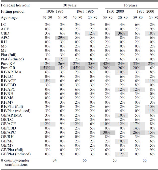
Notes: The MCS procedure is based on a confidence level of 80% and 1000 bootstrapped samples used to construct the test statistic. Within each column, the percentages are calculated as the frequency at which each model is part of the SSM across all country-gender combinations. Each column does not add up to 100% because the SSM can contain several models. The larger the percentage, the darker is the shade marking the cell.
We first consider the results for the reduced age range (59–89). It is clear from both tables that the pure random forests and gradient boosting models (which are both based on the differenced log death rates), denoted “Pure RF” and “Pure GB,” are the better model choices in the majority of cases. For the 30-year forecast horizon and age range 59–89, the pure GB model is part of the SSM in 53% and 45% of the country-gender combinations which means that in 53% and 45% of the country-gender combinations, the pure GB model performs significantly better compared to the models that are not part of the SSM. For the 16-year forecast horizon and age range 59–89, the pure RF model is part of the SSM in 42% and 33% of the country-gender combinations. For these two cases (i.e. the 16-year forecast horizon and age range 59–89), the pure GB and the “GB/APC” model also perform well with frequencies in the range 20–30%.
The age range 59–89 is typically of interest for the pension fund industry. However, other actors, such as life insurance companies, may be more interested in a broader age range including younger ages. Thus, as a robustness check, we also consider results based on the age range 20–89. For the full age range (20–89) and forecast horizon of 30 years, the pure RF model is the better choice in 26% and 35% of the country-gender combinations. For the pure GB model, the frequencies are 15% and 24%. Even though the results for the short forecast horizon of 16 years are more ambiguous with respect to model choice, the pure RF model (and pure GB for the fitting period 1950–2000) is still among the best-performing models.
In general, our results suggest that model selection is strongly dependent on which forecast horizon and age range are considered. The pension fund industry is typically interested in a long-term forecast of future mortality for older ages, while life insurance companies may be more interested in the shorter term for a broader age range. For the short forecast horizon of 16 years, the best model choice is ambiguous: the SSM’s include more models (percentages add up to much more than 100%), while at the same time frequencies are relatively high for many different models. This means that the performances of a relatively large set of models cannot be significantly distinguished from each other in many of the country-gender combinations. In contrast, considering the forecast horizon of 30 years, frequencies are only high for few models, thus giving a clearer indication of which model is the better choice. This suggests that one should be more careful choosing a model when considering longer forecast horizons.
Of course, the choice of model also depends on which country is considered. A thorough investigation of which models are better suited for which countries is left for future research.
5.1. Robustness checks
In Appendix E, we present several robustness checks, neither of which change the results substantially thereby confirming the main results in Table 2.
In Appendix E.1, we show results when forecast performances are compared using RMSE and MAPE (rather than MCS). The results are similar, but since RMSE and MAPE only chooses one model per country-gender combination, frequencies are generally lower.
Appendix E.3 compares forecast performances when the random forests algorithm used for estimating the RF variants of the stochastic mortality models is based on the Poisson deviance loss function (rather than the squared error loss function). The squared error loss function may perform poorly when the number of deaths is small and when volatility of death rates depends on the covariates. To asses the severity of these issues, we carry out forecast comparisons for the 30-year forecast with the fitting period 1961–1989 (both age ranges) using the Poisson deviance loss function for the RF variants of the stochastic models. Details are provided in Appendix E.3. The results obtained are not materially different from the results in Table 2: Percentages increase/decrease by maximum 6 percentage points, except for the RF/ACF model for the reduced age range (59–89) which increases by 9 percentage points.
Appendix E.4 shows results when including/accounting for mortality shocks. The comparison is based on the 30-year forecast horizon with the fitting period 1936–1989 (which include two pandemics and World War II). Compared to the results in Table 2, this weakens the performance of the pure GB model for the reduced age range (59–89) and favors the pure RF model for the full age range (20–89). However, the general conclusion that the pure RF and pure GB models are the best-performing models remain unchanged.
Appendix E.5 shows results when excluding the cohort variable in the set of features for RF and GB estimation and forecasting. The comparison is based on the 30-year forecast horizon with the fitting period 1961–1989 (both age ranges). The results are similar to the results in Table 2. Percentages increase/decrease by a maximum of 6 percentage points.
5.2. Head-to-head comparisons
In order to assess whether random forests or gradient boosting improved the forecast performances of the stochastic mortality models, we also carry out a head-to-head comparison of each of the stochastic mortality models and their RF and GB variants. The comparisons are made for the 30-year forecast and fitting period 1961–1986 for both age ranges. The head-to-head comparisons are presented in Table 3.
Table 3 Head-to-head forecasting comparison based on MCS for 30-year forecast and fitting period 1961–1986.
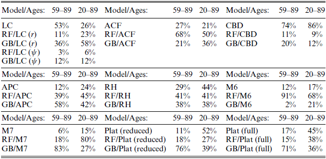
Notes: Within each block, a head-to-head forecasting comparison is performed for the models reported in column 1 of that block. Within each column of each block, the percentages are calculated as the frequency at which each model is part of the SSM across all country-gender combinations.
The results reveal that the choice between a stochastic mortality model and its RF and GB variants is ambiguous which contradicts previous findings, see, for example, Levantesi and Pizzorusso (Reference Levantesi and Pizzorusso2019) and Levantesi and Nigri (Reference Levantesi and Nigri2020). Levantesi and Nigri (Reference Levantesi and Nigri2020) find that RF improve the forecasts of the LC model by comparing out-of-sample RMSE values for Australia, France, Italy, Spain, UK, and USA, ages 20–100. Levantesi and Pizzorusso (Reference Levantesi and Pizzorusso2019) find that both RF and GB improve the LC forecast by comparing out-of-sample RMSE values for Italy, ages 0–100. To better compare our results with those found in the abovementioned papers, we also include the Levantesi and Pizzorusso (Reference Levantesi and Pizzorusso2019) RF and GB variants of the LC model, denoted by “RF/LC (
 $ \psi $
)” and “GB/LC (
$ \psi $
)” and “GB/LC (
 $ \psi $
),” respectively. These models are based on the ratio between the death observations and the estimated number of deaths from the LC model (rather than the model errors used in this paper) and the forecasts are based on the original LC framework (for details, see Levantesi and Pizzorusso, Reference Levantesi and Pizzorusso2019 and Appendix E.2).
$ \psi $
),” respectively. These models are based on the ratio between the death observations and the estimated number of deaths from the LC model (rather than the model errors used in this paper) and the forecasts are based on the original LC framework (for details, see Levantesi and Pizzorusso, Reference Levantesi and Pizzorusso2019 and Appendix E.2).
Comparing the forecast performances of the LC type models shows that the pure LC model outperform or perform equally as good compared to the RF and GB variants in 53% and 26% of the country-gender combinations for the age range 59–89 and 20–89, respectively. In Table A.5 in Appendix E.2 we compare out-sample RMSE values for Italy, France, Denmark, and USA of the LC forecast and its RF and GB variants (both genders and age ranges). Considering the full age range (20–89) and corresponding countries, we arrive at the same conclusions as in Levantesi and Pizzorusso (Reference Levantesi and Pizzorusso2019) and Levantesi and Nigri (Reference Levantesi and Nigri2020). However, for the reduced age range (59–89), the pure LC model is the better model choice in the majority of cases.
Considering a larger range of countries and models, Table 3 shows that RF and GB improve the forecasts of some stochastic mortality models (such as, for example, ACF, M6, M7), while for other models they do not or results are ambiguous. In general, the best model choice is highly dependent on which model and age range is considered. Further, based on the results in Table 2, it is probably also dependent on which fitting period and forecast horizon are considered.
6. Random forests results: Opening the box
The forecasting exercise in the previous section showed that random forests and gradient boosting in their pure form outperform both traditional, stochastic mortality models as well as their random forests and gradient boosting variants. One of the main drawbacks of the traditional models is their inability to model the age pattern of mortality decline in developed countries which is decelerating at younger ages and accelerating at older ages (see Li et al., Reference Li, Lee and Gerland2013). This phenomenon is not an issue for tree-based ML models such as RF and GB, since these models can handle both nonlinear relationships as well as variable interactions. However, since many still consider machine learning models as “black boxes,” the general perception is that the results are difficult to interpret.
The purpose of this section is to provide insights into how random forests results can be interpreted by showing how information can be extracted from the random forests fit (we only consider the random forests results. The gradient boosting results can be interpreted correspondingly and are presented in Appendix G). While the results in themselves are not the main focus, they are used to illustrate how different types of input variables can contribute to understanding past mortality trends and patterns. In light of the model selection criteria listed in Cairns et al. (Reference Cairns, Blake and Dowd2008), this section and the forecasting comparison from the previous section illustrate that pure tree-based models are competitive in terms of being a “good” mortality model with desirable features such as being biological reasonable in long-term dynamics, consistent with historical data, parsimonious, and straightforward to implement.
6.1. Variable importance
The most straightforward way to illustrate how the different input variables affect mortality rates is to show a variable importance plot based on the average decrease in MSE used for choosing the optimal split points. This measure is provided by the randomForest package in R. Figure 1 displays the variable importance for each of the fitting periods for the age ranges 59–89 and 20–89, respectively. A similar measure called relative influence is available for gradient boosting. The relative influence of each variable in the gradient boosting model is plotted in Figure A.4 in Appendix G.
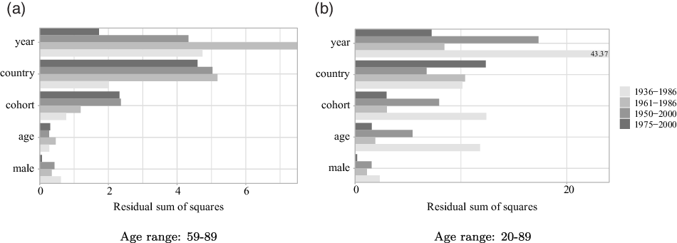
Figure 1: Variable importance for all fitting periods and both age ranges.
year is one of the most important predictors in almost all cases, especially for the fitting periods starting in 1961 or earlier. In addition to capturing changes due to advances in medicine and social progress over time, the year variable in a random forests context is also able to capture periodic breaks like pandemics and war, which the traditional, stochastic mortality models are not built to handle. country is also of high importance, especially when considering the reduced age range 59–89. One explanation why country is more important when considering the reduced age range could be differences across countries in social security systems and access to medical care, which is more demanded at older ages. Later in this section, we analyze in more detail the most frequent country groupings. Surprisingly, cohort is more important than age for all fitting periods, underlining the importance of including a cohort effect when analyzing mortality patterns.
6.2. Frequent variable splits and partial dependence
In the following, we illustrate how to extract information about the most frequent variable splits in the forest. For this purpose, we consider all terminal conditions. The terminal conditions are the variable conditions that constitute each end node in each tree of the forest. Recall that we construct 200 trees and that each tree is constructed using a maximum of 16 end nodes. Thus, the forest consists of 3200 end nodes, and thereby 3200 terminal conditions to be analyzed. The terminal conditions are extracted in R using the inTrees package inTrees. To focus the discussion on how random forests can be a useful tool for analyzing mortality trends and patterns, we only present the results for the fitting period 1961–1986 and age range 59–89 when analyzing the random forests split conditions. Similar results for the other combinations of fitting periods and age ranges can be found in Appendix F.2 while gradient boosting results can be found in Appendix G.
The input variables year, cohort, and age are all numerical, which means that split points are considered as “above and below” conditions. Thus, it is straightforward to plot the split point distribution for each of these variables. The distributions are displayed on the left axis in Figure 2(a), (b), and (c). For the year variable, most splits occur at the beginning of the fitting period. However, there is a small spike in 1969, which can be attributed to the Hong Kong Flu. For the cohort variable, there is a spike at 1900. The distribution of the rest of the cohort split points is skewed toward very old cohorts. The distribution of age has no particular pattern. Figure 2(d) shows the distribution of age split points by gender. The figure reveals that for males more splits occur at higher ages while for females splits are more evenly distributed. The frequencies of gender and age interactions displayed in Figure 2(d) are very low. This is partly due to the relatively low number of terminal conditions, which was limited to 3200 in order to avoid overfitting. However, including more input variables would make it possible to increase the depth of each tree without risking overfitting, thereby making more room for variable interactions. This would, for example, allow us to identify gender and age intervals that were often grouped together, or which year and age intervals that were often grouped together.

Figure 2: Distribution of split points (left axis) and partial dependence (right axis) for the input variables year, cohort, and age. Age range: 59–89, fitting period: 1961–1986.
Figure 2(a), (b), and (c) also display partial dependence plots on the right axis. Partial dependence is another method for understanding the results from random forests (and other ML methods), and they show the marginal effect of one or more variables on the response (for details, see Friedman, Reference Friedman2001). Here, the response is differenced log-mortality rates, that is, changes in the log-mortality rate from one year to the next. The partial dependence of year and cohort show breaks whenever many splits occur and are relatively stable for some ranges of years/cohorts. For age the partial dependence function is downward sloping but without breaks.
The country variable is a categorical variable. The randomForest package in R is built to handle such variables in a suitable way by identifying for each split which categories should go to the left and right (see Appendix B.2 for more details). Categorical variables are very interesting in a mortality context, since an expanded study on individual-level mortality could include categorical variables such as educational level, socioeconomic status, and health status (e.g., health diagnoses). Rather than calculating, for example, average educational level for each country, we here illustrate (using the country variable) how categorical variables in a random forests context can contribute to understanding mortality patterns using the data available at HMD.
We consider the most frequent 4-way country groupings within all terminal conditions containing at most 10 countries. That is, for each terminal condition containing at most 10 countries, we find the four countries that are most often grouped together. These 4-way groupings are displayed in Table 4. The table shows which countries are grouped together, the number of terminal conditions containing at most 10 countries including these four countries, the total number of terminal conditions including these four countries, as well as the total frequency in percentage of the total number of terminal conditions (i.e., 3200). We only display the five most frequent combinations. In Appendix F.1, we show the 50 most frequent combinations. The country combinations in Table 4 only consist of former Soviet Republics or former members of the Warsaw Pact alliance, namely Bulgaria (BGR), Belarus (BLR), Hungary (HUN), Lithuania (LTU), Slovakia (SVK), and Latvia (LVA). Even when considering the 50 most frequent country combinations in Appendix F.1, the country combinations still only consist of former Soviet Republics or former members of the Warsaw Pact alliance. Previous studies on the life expectancy and mortality trends in the Soviet Union have shown that there were little or no improvements from the mid-1950s to the mid-1980s (see, for example, Anderson and Silver, Reference Anderson and Silver1989 and Blum and Monnier, Reference Blum and Monnier1989).
Table 4 Most frequent 4-way groupings of countries. Fitting period: 1961–1986, age range: 59–89.

In Figure 3, we plot the average partial dependence of age by region. For Eastern Europe (Figure 3(b)), which includes countries that are former Soviet Republics or former members of the Warsaw Pact alliance, the relationship between age and mortality changes is very different compared to the other regions. In particular, for Eastern Europe, the pattern is approximately U-shaped while for the other regions it is downward sloping.

Figure 3: Average partial dependence of age by regions. Age range: 59–89, fitting period: 1961–1986.
The above results illustrate the benefits of random forests in terms of analyzing past mortality trends and patterns within and between variables. Since the random forests model places no restrictions on which and how many variables to include, it has a huge potential for providing new insights into the understanding of mortality.
7. Conclusion
This paper illustrates how tree-based machine learning models such as random forests and gradient boosting can be effective tools for studying mortality, both in analyzing past trends and patterns as well as forecasting future mortality. In particular, we show that a pure random forests and pure gradient boosting forecasts of mortality outperform forecasts from traditional stochastic mortality models as well as their random forests and gradient boosting variants. The pure random forests and gradient boosting models are fit and forecast using differenced log-mortality rates, while the machine learning combined variants are fit and forecast using model errors. In total, we produce 31 mortality forecasts based on different models using gender-specific data from the Human Mortality Database covering a large number of countries. Forecast performances are compared for different fitting periods (training sets) and forecast horizons (test sets) using the MCS procedure of Hansen et al. (Reference Hansen, Lunde and Nason2011). In the majority of the country-gender combinations considered within each training and test set combination, the pure random forests and gradient boosting forecasts significantly outperform all other models suggesting that imposing minimal structure on the relationship between the inputs and mortality is better for forecasting purposes. A head-to-head comparison of each stochastic mortality model and its random forests and gradient boosting variants show that tree-based machine learning methods do not necessarily improve the forecast performances of traditional models.
Having demonstrated that the pure tree-based machine learning models can produce more accurate forecasts compared to traditional methods, we show how to “open up the black box” by illustrating how to extract information from the random forests fit which can be used to interpret the results (in-sample results from gradient boosting are shown in the Appendix). In particular, we show the ability of tree-based models to detect patterns within and between variables that are not identifiable by traditional mortality models. One of the things that make tree-based methods particularly advantageous over standard methods is that these models allow for expanding the set of input variables, which would otherwise only include age, period, and cohort. The results show that there are important benefits from using tree-based machine learning models, and that the models have huge potential in terms of providing new insight into understanding past mortality trends and patterns.
Acknowledgments
The author thanks four anonymous referees for their valuable comments and suggestions which helped to improve the manuscript.
Supplementary materials
For supplementary material for this article, please visit https://doi.org/10.1017/asb.2022.11


