The Quantity Theory of Money

The quantity theory of money is a simple, yet powerful, tool for exploring the relationship between money and prices in an economy. It is an old theory, articulated as early as the eighteenth century. Yet, it is still taught in current introductory economics textbooks, where it is regarded as “the leading explanation for how money affects the economy in the long-run” (Mankiw Reference Mankiw2010: 80–94).

The theory, at least a prominent version, takes the equation-of-exchange identity, MV ≡ PY, as expressed in growth rates, lnM + lnV ≡ lnP + lnY, and by assuming that lnV and lnY are long-run constants transforms it into the quantity “theory” of money [lnP = some constant + lnM]; where M = the money supply, V = the velocity of that money’s circulation, P = prices in that money, and Y = traded real output (Boorman and Havrilesky Reference Boorman and Havrilesky1972: 162–81; Bordo Reference Bordo1987; Eatwell et al. Reference Eatwell, Milgate and Newman1989: 1–40; Fisher Reference Fisher1912; Mankiw Reference Mankiw2010: 86–93). In words, the equation-of-exchange identity says that over a given period the total amount of spending (MV) has to be identical to the total value purchased (PY). Growth rates in Y and V are thought to be severely constrained by real forces. Technological and resource constraints, that is, the production possibility frontier, limit how much Y can grow. Institutional and cultural constraints limit how much V can grow. Thus, large movements in M should show up as large movement in P. When applying the quantity theory of money, M is measured in its nominal face value. M’s real value is measured by its relation to P, namely as M/P ≡ Y/V.

The theory is importance because it provides an overarching framework within which the particulars of history must reside. Written histories must be consistent with governing macroeconomic forces, and the quantity theory of money provides a simple framework to assess those forces. In addition, the theory is important because M is under the policy control of governments either directly by being the money issuer or indirectly by how governments organizes their monetary and trade institutions, for example, banking structures and foreign exchange markets. Changes in M, say due to political policy choices, drive other macroforces affecting the economy, in particular P, thus affecting political, social, and economic histories. Many useful historical applications of the quantity theory of money exist in the literature. For the United States, the classics are by Milton Friedman and Anna Schwartz (Reference Friedman and Schwartz1963) for 1867 through 1960, and by Hugh Rockoff (Reference Rockoff1971) for the antebellum period.

In the modern era, applying the quantity theory of money has fallen out of favor for two reasons. First, economists have shifted their focus from large overarching forces to studying the dynamics of smaller business-cycle-type perturbations to the course of macroeconomic variables. Instead of looking at changes in M, economists now focus more on “money demand,” namely on V in the equation of exchange. They model what affects whether the public holds or spends M, which is what V is. Typically, V cannot be directly measured. However, the forces that shift V, derived from economic models, can be measured, such as interest rates, alternative investment vehicles, expectations of future inflation, and consumption versus savings choices (Boorman and Havrilesky Reference Boorman and Havrilesky1972; Eatwell et al. Reference Eatwell, Milgate and Newman1989; Mankiw Reference Mankiw2010: 98–99, 556–64; Sargent Reference Sargent1982; Wallace Reference Wallace1981). Often modern monetary analysis gets mired in technical minutia that abstracts from the bigger picture and so befuddles the general nontechnical reader.Footnote ¹

Second, the quantity theory of money rests on an ability to measure M. A dirty little secret in economic theory is that economists have no way, using the tools of economics, to independently determine what is M and what is not M. Economists simple assume X is M and Z is not M in their models and applications, and that trades in the economy are sufficiently monetized in X that X captures the relational patterns of behavior in the theory corresponding to M. For the nineteenth- and early-twentieth-century US economy, M seems obvious and easy to define and measure, namely it is coins, banknotes, and bank accounts (Friedman and Schwartz Reference Friedman and Schwartz1963; Rockoff Reference Rockoff1971). What constitutes M in the modern economy is less clear, and so harder to measure. The rise of electronic transactions, near monies, and ubiquitous liquid credit/debt instruments that substitute for cash has produced a crisis in determining what M is. For example, the Federal Reserve no longer seriously tracks the US money supply. M in today’s economy is often thought of as more endogenous than exogenous. Thus, modern economists focus instead on money demand (V) and how changes in things such as interest rate policies can influence the path of other macroeconomic variables.

As will be shown in the following text, there is a similar crisis regarding M when applying the quantity theory of money to premodern economies, such as to American colonial economies. For these economies, this is less of a crisis in defining M, which can be easily defined as the paper money issued by colonial legislatures and any foreign specie coins present, than it is a problem created by an undermonetized economy. If most trades do not use M as a medium of exchange, then the equation of exchange is no longer an identity. It breaks down in that movements in Y and P may have little to do with M and V. If the economy is not sufficiently monetized, such that barter transactions dominate, then applications of the quantity theory of money should be consistent with that, namely it should show that there is no statistical relationship between M and P. Such an outcome would have important implications for the M creators, namely the colonial legislatures, in that it reveals the costs and consequences that constrain their money creation actions. Being able to issue more M, and so collect seigniorage (revenue from printing money), without affecting P is a boon to government finance and the general tax payer.

Applying the quantity theory of money to American colonial economies is also important because the colonist thought in, and often articulated, elementary versions of the quantity theory of money. They often remarked that if more paper money was issued than what was needed to execute local trade, the paper money would depreciate, meaning that prices would rise and so lower the purchasing power of the paper money (Davis Reference Davis1964; Grubb Reference Grubb2012; Labaree Reference Labaree1968: 52–53; 1970: 34–35). Colonial historians have often used the quantity theory of money as a lens for viewing colonial economies and what the colonists were up to with paper money (Brock Reference Brock1975: 59; Ernst Reference Ernst1973: xviii, 3–10; McCusker and Menard Reference McCusker and Menard1985: 67, 338, 359). How colonists’ understood the quantity theory of money, however, is not well articulated in the secondary literature, where it is often assumed that the colonists meant a tight relationship between paper M and P. I empirically test the quantity theory of money on the paper money regimes of the American colonies to better understand what the colonists really meant when they talked in quantity theoretic terms yet qualified it with phrases such as “did not exceed the Proportion requisite for the Trade of the Colony” (Labaree 1970: 34–35).Footnote ² This qualifying phrase is consistent with a great deal of nonmonetary barter activity in the local exchange economy.

Paper Money in the British North American Colonies

The British North American colonies were the first Western economies to emit sizable amounts of paper money—called bills of credit. Colonial legislatures printed bills and placed them in their treasuries. They directly spent these bills on soldiers’ pay, military provisions, salaries, and so on. Some colonies loaned bills to their subjects who pledged their lands as collateral. Prior to emitting paper money, the media of exchange used in domestic transactions consisted of barter—typically involving book credit or tobacco, personal bills of exchange, and promissory notes—and foreign specie coins. The composition of this media is unknown, though specie coins were considered scarce. The colonists did not produce specie, as gold and silver were not yet mined there; beside the British Crown did not allow them to mint coins (Grubb Reference Grubb2012). Legislature-issued paper monies became an important part of the circulating medium of exchange in many colonies. No public or private incorporated banks issuing banknote monies existed in colonial America (Brock Reference Brock1975; Grubb Reference Grubb2016a; Hammond Reference Hammond1991: 3–67; Newman Reference Newman2008).

What explains the value and performance of these paper monies and, with it, the inferred political and monetary intentions of colonial legislatures? Applying the quantity theory of money is the obvious and initial place to start to answer these questions. The spending and loaning into circulation of sizable quantities of paper money by colonial legislatures should have affected prices, and thus the real value of the paper monies so emitted, through a quantity-theory-of-money mechanism. Preliminary estimates and casual observations in the prior literature did not always see a clear paper M to P connection, which led some scholars to look for alternative interpretations of the value and performance of colonial paper monies (Wicker Reference Wicker1985: 869–71).

These alternative interpretations still rely on the equation-of-exchange identity. They just focus on different components, such as mechanisms that connect paper M to V or to Y rather than to P, or on currency substitution mechanisms effecting the measurement of M. These alternatives will be explored in detail in the “Discussion” section.Footnote ³ The primary task of this article is to establish more broadly and deeply than has been previously done how the quantity theory of money performs regarding colonial paper monies, namely to establish whether the lack of a connection from paper M to P is a general result or just isolated anomalies (Officer Reference Officer2005: 102). If prior findings are just isolated anomalies, then the alternative interpretations pursued in the recent economic literature are moot.

The initial statistical application of the quantity theory of money to American colonial economies was by Robert Craig West (Reference West1978). He applied the theory separately to four colonies, namely Massachusetts, New York, Pennsylvania, and South Carolina. He set M equal to the paper money placed in circulation by each colony and estimated lnP_t = some constant + lnM_t, including one- and two-year lags of M to capture delayed transmission effects of M on P. The price index (P) was expressed in that respective colony’s paper money unit-of-account and was taken from data on local prices in that respective colony. In the colonies south of New England, he found no systematic relationship between M and P—a puzzling result for the quantity theory of money.

One question that has not been previously addressed is whether these findings are indicative of a general and widespread condition or are limited to a few isolated locations. West (Reference West1978) only tested the quantity theory of money on three of the eight mainland colonies south of New England, comprising only 38.5 percent of the white (free) population therein—as measured in 1770 (Carter et al. Reference Carter, Gartner, Haines, Olmstead, Sutch and Wright2006, 5: 652). In addition, the price indices used by West (Reference West1978) were from the port cities of New York City, Philadelphia, and Charleston, whereas the paper monies used by West (ibid.) circulated at least throughout the colonies of New York, Pennsylvania, and South Carolina.

West (ibid.) confined his study to New York, Pennsylvania, and South Carolina because, at that time, price indices were only available in the secondary literature for these colonies. Since his study in 1978, commodity and exchange rate price information has become available for other colonies. I use these price data to test the quantity theory of money in the mainland colonies south of New England where it has not been previously tested, namely in New Jersey, Maryland, Virginia, and North Carolina. I also retest the quantity theory of money for New York and Pennsylvania because I use these colonies in regional grouping tests. My applications, along with those by West (ibid.), cover seven of the eight mainland colonies south of New England, comprising 95.8 percent of the white (free) population therein. As in West (ibid.), I define M as the paper monies issued by colonial legislatures. The results show whether the failure to find an M to P connection is a widespread and general phenomena or just an isolated outcome.

In the process, I construct more geographically diverse price indices for Maryland and Virginia than the single-port price indices used by West (ibid.). I also use prices for sterling bills of exchange drawn on London to create purchasing power parity (PPP) consistent price measures for each colony, thus providing an additional and alternative specification vehicle. For New Jersey and North Carolina, PPP prices are the only price measures currently available. I also provide improved data on the quantities of paper money in circulation for several colonies, namely for New Jersey, Maryland, and Virginia. Finally, I test the quantity theory of money for regional groupings of contiguous colonies, treating them as one monetary unit. Such has never been done before. Whether colonial borders mattered to paper money circulation in a quantity-theory-of-money framework can be explored with these regional-grouping tests.

Data Limitations

Statistical testing is limited by the availability of annual data on the amounts of paper money in circulation and on commodity prices. Paper money emissions began in 1709 in New Jersey and New York, 1712 in North Carolina, 1723 in Pennsylvania, 1733 in Maryland, and 1755 in Virginia. Once initiated, with minor exceptions, each colony maintained some amount of its paper money in circulation through 1774. Annual data on the amounts in circulation, however, exist for New York only after 1745 and for North Carolina only after 1747. For North Carolina, this evidence ends in 1768 rather than in 1774 as it does for the other colonies. Finally, commodity price evidence for New York only begins in 1748. Thus, the annual data usable for New York span from 1748 to 1774, for New Jersey from 1709 to 1774, for Pennsylvania from 1723 to 1774, for Maryland from 1735 to 1774, for Virginia from 1755 to 1774, and for North Carolina from 1748 to 1768. Out of 308 colony-years when paper money was in circulation, usable annual data for testing the quantity theory of money on a colony-specific level exist for 74 percent of these years—a reasonably comprehensive coverage. The usable data span for various colonial groupings, however, is further limited by the extent of their data overlap.

Besides local commodity price indices, PPP price indices are constructed for each colony. PPP implies that EX_XX = P_XX/P_UK, namely the exchange rate (EX) of colony _XX’s paper money to pounds sterling must equal the ratio of prices in colony _XX, expressed in colony _XX’s paper money (P_XX), to prices in England expressed in pounds sterling (P_UK). Taking the natural log of both sides and rearranging terms yields ln(P_XX) = ln(EX_XX) + ln(P_UK). Data on EX_XX are taken from McCusker (Reference McCusker1978) and Grubb (Reference Grubb2016b: 1220–21), and data on P_UK are taken from Schumpeter (Reference Schumpeter1938: 35). A PPP version of ln(P_XX) is constructed for each colony. It is denoted as ln(PX_XX) in all tables and figures hereafter (see the notes to appendix table 1; online supplementary material).

Using the preceding price and exchange rate data, PPP has been shown to hold for all colonies where colony-specific commodity price indices exist between that colony and England and between that colony and all other colonies with commodity price indices, namely for Massachusetts, New York, Pennsylvania, Maryland, Virginia, South Carolina, Montreal, and Quebec (Grubb Reference Grubb2003: 1786; Reference Grubb2005a: 1346; Reference Grubb2010: 132–35). If PPP holds for these colonies, then it is reasonable to assume that it holds for New Jersey and North Carolina when using the same data sources. Using PPP price indices in the quantity-theory-of-money framework provides an alternative check on the results using commodity price indices for the colonies of New York, Pennsylvania, Maryland, and Virginia. The exchange rates for constructing PPP prices come from the prices in local paper money for purchasing sterling bills of exchange drawn on London (McCusker Reference McCusker1978). As such, PPP prices can be considered as the local prices of sterling bills of exchange drawn on London, that is, not that different conceptually from using local wheat or tobacco prices to create a commodity price index.

The commodity price indices for New York and Pennsylvania are the same as used by West (Reference West1978), namely from Bezanson et al. (Reference Bezanson, Gray and Hussey1935: 6, 433) and Cole (Reference Cole1938: 11, 120–21). These price indices consist of the unweighted averages of 20 commodities for Pennsylvania and 15 commodities for New York. These commodities are import and export goods in the port cities of Philadelphia and New York City, respectively.

For Maryland and Virginia, I construct unweighted price indices from annual data on the prices of wheat, corn, and tobacco. While these indices involve fewer commodities than the indices for Pennsylvania and New York, these three commodities were the most ubiquitously traded local goods in Maryland and Virginia. For Maryland, Paul Clemens (Reference Clemens1980: 225–27) used prices found in probate inventories held in the Maryland Hall of Records for deceased white residents from Kent and Talbot counties to construct annual average prices for wheat, corn, and tobacco. I combine his three-price series into one unweighted arithmetic price index for Maryland.

For Virginia, Lorena Walsh (Carter et al. Reference Carter, Gartner, Haines, Olmstead, Sutch and Wright2006, 5: 682–87) used prices found in planter and merchant inventories, account, and letter books, along with prices found in deceased white resident probate inventories, to construct annual average prices for wheat, corn, and tobacco. The tobacco prices were from the York and Rappahannock river basins, the corn prices from the York River basin, and the wheat prices from the James River basin. I combine these three-price series into one unweighted arithmetic price index for Virginia. The price indices I construct for Maryland and Virginia cover a wider geographic area within each colony, and so are likely more representative of price movements within these colonies, than the single-port price indices used by West (Reference West1978) for Pennsylvania and New York.Footnote ⁴

Data Patterns and Estimation Procedures

The data are presented in appendix table 2 (see online supplementary material) and displayed by individual colony in figures 1, 2, 3, 4, 5, and 6. The figures show that movements in the quantities of paper money were not small. If these movements were only, say, 5, 10, or 20 percent up or down over time, then finding a systematic relationship between paper money and prices might be difficult given noisy price data. The movement in the quantities of paper money in all six colonies, however, were large—doubling, tripling, or even quadrupling up or down over short spans of time. Even given noisy price data, applying the quantity theory of money should reveal substantial positive relationships between movements in paper money and prices. However, the figures also show that paper money and prices do not track each other well. A poor statistical fit seems likely.

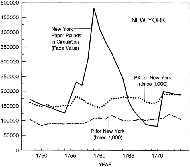
Figure 1 New York paper money in circulation and New York prices.

Sources: Appendix table 2 and text.

Notes: P = commodity price index and PX = purchasing power parity price index. These price indexes are rescaled to fit on the same vertical axis as the quantity of paper money in circulation.

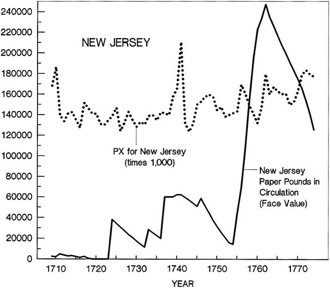
Figure 2 New Jersey paper money in circulation and New Jersey prices.

Sources: Appendix table 2 and text.

Note: See the notes to figure 1.

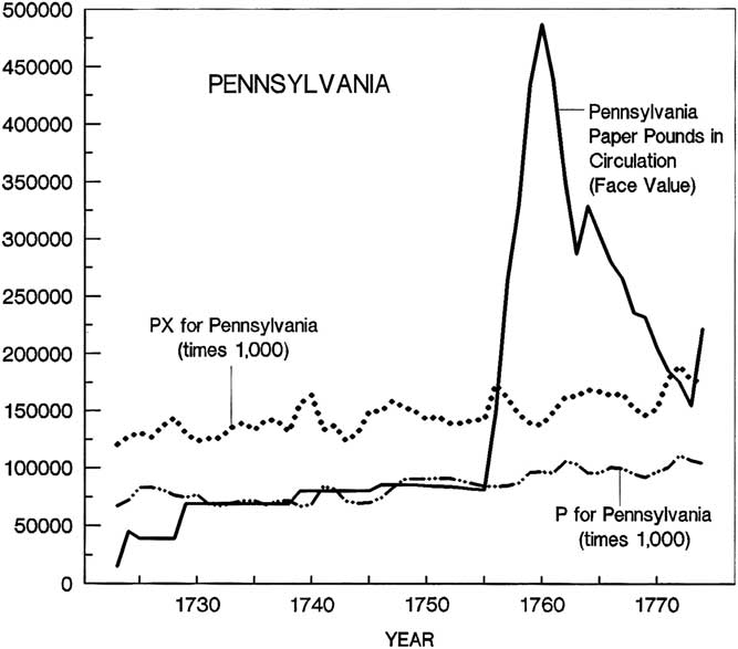
Figure 3 Pennsylvania paper money in circulation and Pennsylvania prices.

Sources: Appendix table 2 and text.

Note: See the notes to figure 1.

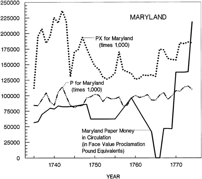
Figure 4 Maryland paper money in circulation and Maryland prices.

Sources: Appendix table 2 and text.

Notes: See the notes to Figure 1. Proclamation value was 1.33 paper pounds being equal to 1 pound sterling, see the notes to appendix table 1.

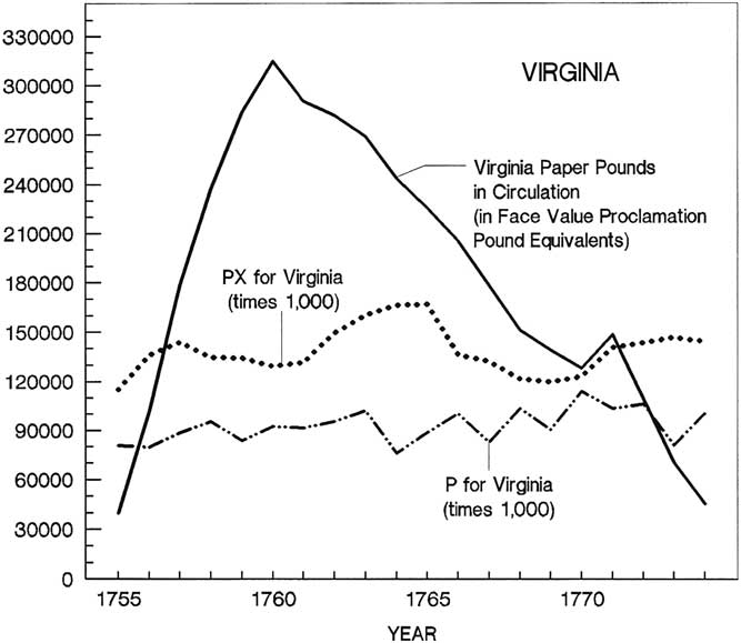
Figure 5 Virginia paper money in circulation and Virginia prices.

Sources: Appendix table 2 and text.

Note: See the notes to figure 4.

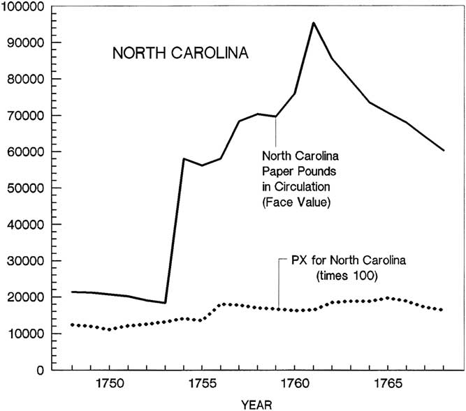
Figure 6 North Carolina paper money in circulation and North Carolina prices.

Sources: Appendix table 2 and text.

Note: See the notes to figure 1.

With the exception of Maryland, the figures also show relatively large expansions and then contractions in the quantities of paper money in circulation in all the colonies during the Seven Years’ War (1754–63). Starting in 1754–55, new paper money emissions increased. These emissions accumulated into large quantities in circulation that peaked around 1760. Thereafter, more paper money was removed from circulation than was newly emitted, causing the quantity of paper money in circulation to decline sharply from 1760 through 1774.

These large movements in the quantities of paper money in circulation, caused by how each colony financed their participation in the Seven Years’ War, gives enough variation in the data to allow confident statistical testing even when the data spans are relatively short. Wicker (Reference Wicker1985) used this Seven Years’ War period to note that the movements in the quantities of paper money and prices in New York, Pennsylvania, and South Carolina appear unrelated between 1754 and 1765. He did not, however, statistically test his observation, nor embed the data in longer time spans, nor test colony-grouping combinations, nor consider colonies beyond those considered by West (Reference West1978). The analysis here is an expanded and generalized statistical test of Wicker’s (Reference Wicker1985) impressionistic findings regarding the Seven Years’ War period.

Finally, understanding the progress of paper money emissions and the amounts remaining in circulation, and how they related to prices, is important for understanding the subsequent history of financing the American Revolution with paper money. The colonist’s most recent experience with large-scale war finance using paper money was during the Seven Years’ War. This experience provided an expectation as to how prices would behave if the revolution was financed in the same manner, thus explaining the Second Continental Congress’s initial paper money choices in 1775.

The quantity theory of money is a theory about magnitudes. When estimating relationships between paper money and prices, focusing solely on statistical significance is misplaced. At best, statistical significance is a necessary, but not a sufficient condition, for the theory to be a useful explanatory tool. When estimating lnP_t = a + blnM_t, the quantity theory of money holds perfectly if b = 1 and doesn’t hold at all is b = 0. No one expects the theory to hold perfectly. Systematic short-run, business-cycle-like movements in V and Y, namely deviations from their assumed constant growth values of lnV and lnY, are expected (Fisher Reference Fisher1912; Lucas Reference Lucas1980). Such movements, however, are limited, especially in the face of large changes in M. Resource, technological, and production constraints limit how much Y can move, and transactions costs limit how much V can move. Y or V doubling or tripling over a short span of years stretches credulity. Given sizable movements in M, b should be relatively large, much closer to 1 than to 0 for the quantity theory of money to be a useful theory for explaining the value and performance of M. Therefore, the magnitude of b, and whether it is unbiased and consistently estimated, is the key concern.Footnote ⁵

To have comparable results, I use the econometric specifications in West (Reference West1978: 4), namely lnP_t = a + blnM_t, including regressions with one- and two-year lags of M, where M = the paper money supply. See also comparable specifications in Grubb (Reference Grubb2004: 349) and Rousseau (Reference Rousseau2007: 267). Out of the 90 regressions run on the six individual colonies and their various groupings, 77 exhibit serial correlation (appendix table 1; see online supplementary material). Statistical theory establishes that coefficients are unbiased and consistently estimated in the presence of serial correlation, but the standard errors are biased down, thus overstating statistical significance (Maddala Reference Maddala1977: 281–83; Pindyck and Rubinfeld Reference Pindyck and Rubinfeld1998: 159). Because the focus of the quantity theory of money is on estimating the magnitude of b as an unbiased and consistent coefficient, regressions uncorrected for serial correlation still have a valid interpretation regarding b. If b is close to zero, it doesn’t matter whether serial correlation is corrected, the quantity theory of money is not telling us much about the value and performance of colonial paper monies. In addition, if b is not statistically significant, then we can be certain that it is not statistically significant whether serial correlation is corrected. Regressions uncorrected for serial correlation still have a valid interpretation for statistically insignificant coefficients.

Correcting for serial correlation is only relevant to the quantity theory of money if b is both relatively large and statistically significant. In such cases, correcting for serial correlation is required to avoid erroneously finding statistical significance where it is not. The regressions in appendix table 1 (see online supplementary material) show that these conditions are not manifest in any of the regressions.

Nevertheless, for the 77 regressions that exhibit serial correlation, I report regressions that correct that serial correlation by adding lags of the dependent variable until Durbin’s Alternative Test for serial correlation fails to reject the hypothesis of no serial correlation. These regressions are reported immediately below the uncorrected regressions in appendix table 1 (ibid.). The effect of lagged P on these quantity-theory-of-money regressions has an interesting interpretation for the colonial economy that is explored in “Discussion.”

Regression Results

Table 1 summarizes the results from the regressions reported in appendix table 1 (ibid.) that are uncorrected for serial correlation. For individual colony-specific tests, only 7 of the 30 regressions have statistically significant coefficients on M—again a biased high count. Only Pennsylvania and North Carolina have these statistically significant coefficients. Thus, the lack of any relationship between P and M for New York, New Jersey, Maryland, and Virginia can be accepted with confidence. For Pennsylvania and North Carolina, the magnitude of the relationship between P and M for the statistically significant coefficients is trivial. A 10 percent increase in M corresponds to a 1.1 and 2.1 percent increase in P, respectively.

Table 1 Regression results uncorrected for serial correlation

Sources: Appendix table 1 (see supplementary material).

Notes: See the notes to appendix table 1. NY = New York, NJ = New Jersey, PA = Pennsylvania, MD = Maryland, VA = Virginia, and NC = North Carolina. Statistically insignificant coefficients on M are evaluated as zeros—indicated by dashes in the table.

On the individual colony level among the mainland colonies south of New England, the lack of positive statistically significant and quantitatively meaningful relationships between the quantities of paper monies in circulation and prices are a general and widespread phenomena, and not just confined to the port cities of New York City, Philadelphia, and Charleston. As such, the quantity theory of money is not a useful tool for explaining the value and performance of individual colony paper money regimes for the colonies south of New England. Correcting for serial correction cannot change this conclusion.

Colonies south of New England did not make the paper money of their neighboring colonies a legal tender within their own jurisdictions. The paper money of each colony was uniquely and easily distinguishable (Newman Reference Newman2008). Nevertheless, some scholars have asserted that paper monies circulated across colonial borders, particularly between New York, New Jersey, and Pennsylvania, and between Maryland and Pennsylvania.Footnote ⁶ One explanation for the lack of a statistical association between paper money and prices at the individual colony level is that the paper money supply is incorrectly measured. The relevant paper money supply might be the combination of the paper monies of contiguous colonies.

Table 1 summarizes the results from the regressions in appendix table 1 (see online supplementary material) for the combined paper money supplies of various groupings of colonies. All contiguous pairs of colonies in the sample are tested as though the pairs are one monetary unit. The same is done for all contiguous triplets of colonies in the sample, and for four and five contiguous groupings running from New York south. The price variables are the unweighted average of the commodity price indices, and the unweighted average of the PPP price indices, available for each grouping. Paper money values are converted to be in comparable units, namely proclamation values, and price indices are set to 100 in the same year for the colonies so grouped together.

For contiguous pairs of colonies treated as a single monetary unit, 9 out of 30 regressions have statistically significant coefficients on M—again a biased high count. All but one are due to including Pennsylvania or North Carolina, with their individual colony-level statistically significant coefficient on M, in the pair. As such, little is gained by treating neighboring colonies as one monetary unit. Only the New York–New Jersey pair adds a new statistically significant positive coefficient on M.

The magnitude of the relationship between P and M for the statistically significant coefficients among the colonial pairs is trivial. A 10 percent increase in M corresponds to an average increase in P of between 1.3 and 1.9 percent—the maximum being 2.8 percent. The hypothesis that contiguous pairs of colonies formed one monetary unit, and that such mattered to prices, finds little support in the evidence. As such, the irrelevance of cross-border circulation of paper monies among contiguous pairs of colonies cannot be rejected with confidence.

Table 1 also summarizes the results from the regressions in appendix table 1 (ibid.) for contiguous triplet colonial groupings, under the hypothesis that the monetary unit might be larger than just neighboring colonies. Out of 18 regressions, only three have statistically significant coefficients on M—again a biased high count. All three are due to including Pennsylvania or North Carolina, with their individual colony-level statistically significant coefficient on M, in their grouping. Thus, nothing is gained by treating contiguous triplets of colonies as one monetary unit. In addition, the magnitude of the relationship between P and M for the statistically significant coefficients among the triplets is trivial. A 10 percent increase in M corresponds to an average increase in P of 2.1 percent—the maximum being 3 percent.

Lastly, table 1 summarizes the results from the regressions in appendix table 1 (ibid.) for contiguous four and five colonial groupings, spanning from New York to Maryland and from New York to Virginia, under the hypothesis that the monetary unit might be even larger than just contiguous triplet colonial groupings. Out of 12 regressions, only three have statistically significant coefficients on M—again a biased high count. All three are due to including Pennsylvania, with its individual colony-level statistically significant coefficient on M, in their grouping. Thus, nothing is gained by larger contiguous groupings of colonies as one monetary unit. In addition, the magnitude of the relationship between P and M for the statistically significant coefficients among these larger groupings is trivial. A 10 percent increase in M corresponds to an average increase in P of 0.9 percent—the maximum being 1.8 percent. The hypothesis that the relevant monetary unit extends across numerous contiguous colonies, and that such mattered to prices, finds little support in the evidence. Again, the irrelevance of cross-border circulation of paper monies among the colonies south of New England cannot be rejected with confidence.

The classical quantity of money assumes that lnV and lnY are long-run constants. The constant term in the regressions in appendix table 1 (ibid.) estimates the difference in these long-run constants, namely [lnV – lnY]. In all 90 regressions this constant term is positive, relatively large, and statistically significant. In 35 out of the 77 regressions that were corrected for serial correlation this constant term remains positive and statistically significant—the biggest exception being for New York and for any group that includes New York. Therefore, the conclusion that lnV > lnY in terms of their long-run growth rates can be accepted with confidence. For V to be growing at a faster rate on average than Y indicates that domestic transactions were becoming increasingly monetized with paper money.

Finally, the magnitude of the constant term creates an accounting problem. The long-run growth of colonial Y per capita per year for the relevant period is thought to be between 0 and 0.6 percent (Egnal Reference Egnal1998: 43; Mancall and Weiss Reference Mancall and Weiss1999: 18, 36; McCusker and Menard Reference McCusker and Menard1985: 53–58). Thus, the long-run yearly growth rate in Y is approximately the same as the long-run yearly growth rate of the population. Yearly population growth rates for the relevant period are approximately 6 percent for New York, 8 percent for New Jersey, 14 percent for Pennsylvania, 3 percent for Maryland, 5 percent for Virginia, and 7 percent for North Carolina (derived from Carter et al. Reference Carter, Gartner, Haines, Olmstead, Sutch and Wright2006, 5: 652). Using these numbers for lnY and setting [lnV – lnY] equal to the constant terms in the regressions in appendix table 1 (see online supplementary material) yields what might be considered impossibly high values for lnV. This observation raises the possibility of an accounting problem in the equation of exchange identity. This issue is taken up next.