2.1 Terminology and notation

I will attempt to adhere to the notation and terminology in NW. In particular, I assume that the definition of states, consequences and (Savage) acts are understood. Prior and conditional preferences given an event E are denoted by ≽ and ≽_E respectively.

Throughout this paper, dynamic-choice problems will be represented more concretely by means of decision trees. I shall refer to nodes, actions available at a node, and terminal nodes; these terms all have standard meaning, but an example may still help. Following NW, we consider a dynamic version of the three-colour-urn Ellsberg example. The underlying urn contains 30 black balls and 60 red or yellow balls, in unspecified proportions. If the DM chooses L, then he gets to choose again between u and d without further information. If, however, the DM chooses R, she gets 10 in case the ball drawn is yellow; otherwise, she learns that the ball drawn is black or red, and again gets to choose between u and d. Figure 1 corresponds to NW's Figure 5; I eliminated “information sets” by depicting the DM's initial choice before the (partial) realization of the uncertainty. Filled circles (•) denote decision nodes, and empty ones (○) indicate chance nodes, where uncertainty is (partially) resolved. The initial node is represented by a “fatter” filled circle. The actions available at the initial node are L and R; following L, the DM chooses again between the actions u and d, after which all uncertainty is resolved. Following R, uncertainty is partially resolved: the DM learns whether the ball drawn is yellow or not. If it is, she obtains a payoff of 10; otherwise, she gets to choose between u and d.

Figure 1. A decision tree (NW fig. 5).

To describe the DM's intended choices throughout the tree, we consider the notion of a plan of action, or simply “plan”: a specification of actions at all decision nodes that are not ruled out by prior actions.Footnote ¹ In Figure 1, the possible plans of action are (L, u), (L, d), (R, u) and (R, d).

A plan of action is, strictly speaking, not a Savage act; we can, however, apply the principle of reduction to “map” it to a Savage act. Specifically, for each possible state, we trace out the path through the tree generated by the plan, until a terminal node is reached and the resulting consequence is determined. For instance, the plan (L, u) corresponds to the act (10, 0, 10), where (x, y, z) is the act that delivers prize x in state b, prize y in state r, and prize z in state y. Similarly, the plan (R, d) maps to the act (0, 10, 10).Footnote ² In the tree of Figure 1, the actions u and d at the non-initial decision nodes also map to acts in a natural way. Specifically, the action u at the decision node following L maps to the act (10, 0, 10); the action u at the node following R and the event {b, r} instead maps to a partial act (10, 0, *), where we do not specify the outcome in case the ball drawn is yellow because, at that node, the ball is known to be either black or red.

2.2 Dynamic choice with EU preferences

As noted above, static EU preferences come equipped with a “built-in” theory of dynamic choice. Among its many virtues, Savage's sure thing principle provides the behavioural underpinnings for the usual definition of conditional probabilities (i.e. Bayesian updating). To elaborate, given a (non-null) event E, stipulate that an act f is preferred to another act g given E, written f ≽_Eg, if and only if f E h ≽ g Eh (in the usual notation for composite acts). For this definition of conditional preferences to be well-posed, it must be the case that we cannot find two acts h, k such that f Eh ≽ g Eh and f Ek ≺ g Ek: the sure thing principle is precisely the statement that two such acts cannot be found. In other words, the sure thing principle can be restated as follows: the above definition of conditional preferences (henceforth “Savage's rule”) is well-posed.Footnote ³ Finally, it is immediate to verify that, if P is the probability that represents prior preferences jointly with a utility function u, then f ≽_Eg if and only if E_P[u ○ f|E] ≥ E_P[u ○ g|E].

Complementing this construction of conditional preferences with the reduction assumption, we thus obtain a complete theory of behaviour in dynamic decision problems. Furthermore, dynamic EU behaviour enjoys two key properties.

• • Consequentialism: preferences at a given decision node in the tree are fully determined by the residual uncertainty and the payoffs that may be obtained starting from the node under consideration. In other words, subtrees can be analysed independently of the whole tree; foregone payoffs, unrealized events, and actions taken in the past, as well as intended future actions, do not influence conditional preferences.

• • Dynamic Consistency: at any decision node, the DM will be willing to carry out the plan of action that she determined to be optimal ex ante. In other words, if the DM deems a given action available at a node to be optimal when she considers the entire decision tree, she continues to prefer it to all other available actions upon actually reaching that node.

These properties are both attractive and convenient: for instance, they provide the basis for backward induction and dynamic programming, two techniques whose practical importance simply cannot be overstated.

Both properties descend from Savage's updating rule and the sure thing principle. In fact, it turns out that Consequentialism and Dynamic Consistency are equivalent to Savage's rule and the sure thing principle: see e.g. Ghirardato (Reference Ghirardato2002), or Siniscalchi (Reference Siniscalchi2009, §4).

2.3 Ambiguity and dynamic choice: three approaches

This last observation is the crux of the matter. As is well-known, ambiguity, as manifested for instance in the Ellsberg paradox, entails precisely a violation of the sure thing principle. It then follows that, if preferences are ambiguity-sensitive, then either Consequentialism or Dynamic Consistency (or both) must fail in some respect. A recent, illuminating discussion is provided by Hanany and Klibanoff (Reference Hanany and Klibanoff2007b); see also Ghirardato (Reference Ghirardato2002) and Siniscalchi (Reference Siniscalchi2009). Furthermore, it is well-known that a similar statement holds for non-expected utility models of choice under risk: see e.g. Hammond (Reference Hammond1988, Reference Hammond1989), Machina (Reference Machina1989), Karni and Safra (Reference Karni and Safra1989), and Karni and Schmeidler (Reference Karni and Schmeidler1991). The underlying idea is similar: Consequentialism and Dynamic Consistency are separability properties, and so are the sure thing Principle (in the setting of choice under uncertainty) and the Independence axiom (for choice under risk); thus, one should expect a tight connection between them (under the reduction assumption: see Segal, Reference Segal1990).

To sum up, the modeller interested in ambiguity can essentially pick any two out of three ingredients: full generality in the representation of ambiguity attitudes, Consequentialism, or Dynamic Consistency. She cannot have all three (however, she can have a little bit of each). This motivates the title of this paper. It is important to reiterate that this “impossibility result” is, essentially, a folk theorem, as the above references indicate; versions of the examples presented by NW are also well-known.

The subjective ambiguity literature has explored several combinations of these three ingredients. The approach pioneered by Epstein and Schneider (Reference Epstein and Schneider2001) has proved most popular in applications. It maintains Consequentialism and restricts, but does not drop, Dynamic Consistency. By necessity, this approach also restricts the range of attitudes toward ambiguity that may be represented. I do not discuss this approach in this paper, but NW do so in §3.4. Hanany and Klibanoff (Reference Karni and Schmeidler2007b) advocate dropping Consequentialism; their approach is discussed by NW in §3.3, and here in Section 4. The advantage is that one maintains the full power of Dynamic Consistency, and full generality in the representation of ambiguity attitudes; the drawback is that conditional preferences must depend upon the entire “context” of the decision, i.e. the full tree and the intended plan of action.

Yet another approach was advocated by Siniscalchi (Reference Siniscalchi2009) in the present context, but is inspired by earlier work in the context of certain and risky choice by Strotz (Reference Strotz1955–6), Gul and Pesendorfer (Reference Gul and Pesendorfer2005) and Karni and Safra (Reference Karni and Safra1989) among others. It retains Consequentialism and drops Dynamic Consistency in its entirety, thereby allowing for full generality in the representation of ambiguity attitudes. To resolve conflicts among preferences at different decision points, this approach adopts the principle of sophistication (or more precisely Consistent Planning). I devote Section 2.4 to this approach, because I find the discussion in NW (§3.2) lacking in detail and, as a result, ultimately misleading.Footnote ⁴

The details of these approaches will be considered below. However, it is important to emphasize that, in each case, one or more properties of dynamic EU behavior are consciously and purposely relaxed, and a coherent theory of dynamic choice is assembled out of the remaining properties. By “coherent” I mean a theory wherein every preference can be rationalized in an internally consistent way, invoking the properties that are maintained and pointing to those that are relaxed. For instance, NW complain that a DM who follows the approach advocated by Hanany and Klibanoff (Reference Hanany and Klibanoff2007b) ends up “distorting” her beliefs depending on her prior actions, so as to maintain Dynamic Consistency; they assert that “[t]here is no independent motivation for why a rational decision maker would ever engage in such distortions”. But allowing conditional preferences to depend upon past actions (and the intended continuation plan) is the very nature of the non-consequentialist approach advocated by Hanany and Klibanoff. Thus, for a DM who follows their approach, it is not at all “irrational” to engage in such “distortions”: it is precisely what she is supposed to do!

Of course, it is perfectly legitimate for NW to express their own subjective distaste for such distortions. However, seen in this light, NW's “critique” is revealed for what it is – a statement about their own modelling preferences. This turns out to be true for almost all of their critical observations.

2.4 Introspection-proof preferences

Before tackling sophistication and non-consequentialist choice, I offer a general observation on the basic idea of “rationality” in the present context.

As NW note, there is a bit of circularity in discussing the rationality of preferences in the context of an axiomatic decision model (or, equivalently, one that can be provided with axiomatic foundations): the axioms themselves are meant to tell us what is “rational behaviour”.

Here, I differ only slightly from NW. In my view, for a preference relation to be deemed “rational”, it must be at least transitive and monotonic (i.e not leading to strictly dominated choices). For this reason, I concur with NW's assessment of naiveté (§3.1): it cannot be considered a rational theory of dynamic behaviour.

However, arguing about other axioms is quite a bit more delicate. To circumvent this difficulty, NW propose that preferences may be deemed “rational” if they are immune to introspection. That is, upon reconsidering the preferences she expresses in a given experimental or actual decision setting, the DM is not ashamed of them, and will not want to revise them.

I find this approach eminently reasonable, and would actually push it even further than NW do. For the purposes of understanding the issues at hand, the decision theorist should only take into account preferences that are immune to introspection. In other words, we should first give the DM an opportunity to “rethink her preferences”, and proceed with the analysis only after she has done so.

This is not just a minor quibble. Suppose, for instance, that even after careful reconsideration, the DM's prior and conditional preferences are dynamically inconsistent. In particular, the DM may have constructed her preferences using some model of choice under ambiguity, augmented with an updating rule; if so, we assume that the DM has taken the time to “see how she feels about them”, and ultimately decided that those are, in fact, her preferences. If this is the case, then we as decision theorists simply have to accept the DM's dynamic inconsistency. We can, of course, express our own subjective judgment as to whether we would feel ashamed of such inconsistency, even if the DM does not. But, in doing so, we have to be very clear on one fact: we are expressing our own preferences. Otherwise, we would not be identifying “rationality” with “introspection-proofness”: we would be imposing our own canons of reasonable behaviour onto the DM.

There is a further corollary to this methodological stance. If we are trying to criticize the way this DM copes with her dynamic inconsistency, our arguments cannot boil down to lamenting the fact that the DM is dynamically inconsistent! I will refer back to this observation several times in the following.

3.1 NW's example: a more precise analysis

I shall now focus on NW's discussion of sophisticated choice and “information aversion”. The starting point of their analysis is the observation that (as is well-known) if prior and conditional preferences are dynamically inconsistent, one needs to stipulate how the DM resolves this conflict. NW quickly discard the naive-choice approach, and I have nothing to add to their critique. They then turn to sophisticated choice. In a two-period decision problem, a sophisticated DM holds correct (prior) “beliefs” about her own time-2 choices, and takes them into account when choosing an action at time 1. NW mainly discuss the example reproduced in Fig. 1 above (Fig. 5 in their paper), and I will for the most part stick to their example. I also discuss richer and more insightful examples in §3.3 below.

NW consider a DM with ex-ante MEU preferences, with a set of priors C consisting of all probabilities P on the state space {b, r, y} with P(b)=, and prior-by-prior updating. Observe that, for all P ∈ C, P(b|{b, r}) ∈ [, 1]. Such preferences are consistent with Ellsberg behaviour in the static three-colour urn problem, and are dynamically inconsistent.

As I noted above, NW's discussion of this example in §3.2 is a bit too informal. Unfortunately, this lack of precision conceals certain aspects of the problem that are, in my view, quite crucial. I will flesh out their discussion, using the language introduced in Section 2. For simplicity, “time 1” refers to the time when the DM chooses between L and R, and “time 2” refers to the time when, if necessary, the DM chooses between u and d.

As noted in §2, every plan of action maps to a Savage act in a natural way. NW adopt the reduction principle, also discussed in §2, and we shall do so here as well. This induces a preference ordering over plans at time 1. In particular, we can say that

But what do these time-1 preferences over plans actually mean? Strictly speaking, the DM only chooses between L and R at time 1: she does not also choose between u and d. If she did, then Figure 1 would not be a correct depiction of the situation. Again, in the problem under consideration, the choice between u and d is made at time 2, not at time 1, and right now we are concerned solely with the DM's time-1 preferences.

This seemingly minor quibble is actually the key to reconciling dynamically consistent behaviour with dynamically inconsistent preferences. A plan of action such as (L, u) can be interpreted as a subtree of the tree in Figure 1, in which the only choice available at time 1 is L, and the only choice available at time 2 is u. Of course, the resulting subtree does not depict a very interesting “decision” problem: no actual choice need be made. But that's exactly the point: a plan of action ensures commitment to a specific set of contingent choices. By way of contrast, no such explicit commitment ability is available in the tree of Figure 1 – not at time 1, and not at time 2 following either time-1 action.

Thus, the DM's time-1 “Ellsbergian” preference for the plans (L, d) and (R, d) over the plans (L, u) and (R, u) translates to the following statement:

The important point here is that the DM's time-1 preferences for commitment to d over commitment to u are logically quite distinct from her actual time-2 preferences over u vs. d. In fact, dynamic consistency is precisely the assumption that time-1 “commitment preferences” coincide with actual time-2 preferences; if these objects were not logically distinct, dynamic consistency would be a tautology.

We are thus led to consider the DM's actual time-2 preferences. Consider first the easy case of preferences at the decision node following the time-1 choice of L. Again, NW are a bit loose here, but the spirit of their discussion is right. As noted in Section 2, the actions u and d at that node map to the Savage acts (10, 0, 10) and (0, 10, 10) respectively, just like the time-1 plans (L, u) and (L, d). Furthermore, the DM receives no information between time 1 and time 2 if she chooses L. Hence, following L, the DM is essentially still using her time-1 preferences over acts, and the reduction assumption “buys” us dynamic consistency: the Ellsbergian DM will continue to strictly prefer d to u.

Another way to interpret this is to say that, if the DM chooses L at time 1 in the tree of Figure 1, and wishes to follow L with d, the additional commitment power afforded by the plan (L, d) (that is, the commitment ability she would have if we simply removed action u following L) is not valuable: at time 2, this DM will be able to carry out her intended action d even if, so to speak, her hands are not tied.

Now consider the more interesting case of the DM's preferences at the node following the time-1 choice of R. Again apply reduction, and recall that now u and d now map to the “partial” Savage act (10, 0, *) and (0, 10, *) respectively. For the running example of MEU preferences and prior-by-prior updating, this implies that the DM strictly prefers u to d.

We are now getting to the heart of the matter. We noted above that this DM strictly prefers (R, d) to (R, u); however, as we just found out, once she chooses R, she then strictly prefers u to d. Her time-1 preferences over commitment to u vs. d following R are different from her actual time-2 preferences. Again, there is no logical inconsistency here, because we are talking about preferences over different objects. However, Dynamic Consistency is clearly violated.

It is worth reminding the reader that we imagine that the DM has already been given a choice to reconsider her preferences. Thus, despite NW's editorializing, there is no further opportunity for her to feel “ashamed” of her preferences.

Let's now relate these preferences to sophistication and the value of information. A sophisticated DM will reason as follows:

Strotz (Reference Strotz1955–6, p. 173) said it best: the DM chooses “the best plan among those [s]he will actually follow”. To elaborate, the sophisticated DM correctly anticipates her time-2 preferences, and incorporates them as an “implementation” constraint into her time-1 decision problem.

The action R causes the choice between u and d to be made after learning that the ball drawn is black or red, whereas the action L conveys no further information. Thus, the sophisticated DM under consideration seemingly chooses not to receive information by opting for L at time 1. NW follow an illustrious, but still (in my view) unfortunate traditionFootnote ⁵ in referring to this as a manifestation of “information aversion”.

3.2 The trade-off between value of information and value of commitment

However, the more detailed analysis of the tree in Figure 1 provided above reveals that this conclusion is not warranted. The noted choice of L is inconclusive as regards the DM's attitudes toward information. Moreover, at best, the tree in Figure 1 is too simple to gain a full understanding of information acquisition under ambiguity.

The reason is that the actions L and R differ in two dimensions. It is certainly true that, as noted above, R causes the choice between u and d to be made after learning that the ball drawn is black or red, whereas the action L conveys no further information. However, R also causes the choice between u and d to be made on the basis of the DM's updated preferences over acts, whereas the action L ensures that the corresponding choice will be made based upon the DM's prior preferences over acts. Thus, by choosing L, the DM can be certain that, come time 2, she will be able to implement the plan that she deems optimal at time 1; equivalently, action L enables the DM to commit to her intended course of action. On the other hand, by choosing R, the DM recognizes that she will not be able to do so – and indeed she will end up choosing an action that, from the perspective of time 1, is undesirable.

NW are rather fond of invoking “basic economic reasoning” throughout their critique, so I shall do the same here. Like any good economic agent, our DM must trade off the superior information provided by R with the ability to commit to her intended plan afforded by L. A priori, this trade-off could be resolved either way; for the preferences under consideration, it so happens that commitment is the overriding concern, and this leads to the choice of L at time 1.

Of course, if the DM was dynamically consistent, there would be no trade-off, because commitment would simply not be an issue regardless of whether or not information is obtained. But, once again, recall that we are taking dynamic inconsistency as given: when we arrive on the scene of the (alleged) crime, the DM has already been given the opportunity to reconsider her preferences, and has chosen not to do so.

Because the choice of L over R reflects a trade-off between the value of information and the value of commitment, it cannot be taken as evidence of “information aversion”. An analogy with risk attitudes may be useful. Consider the random variables X and Y, where X yields the prizes 10 and 0 with equal probability, and Y yields 2 for sure. Suppose the DM prefers X to Y. Could we then conclude that this choice is driven by risk appeal? After all, X is risky and Y is certain! The answer is clearly negative, because the DM may simply be trading off risk and return; for instance, a risk-averse DM with square-root utility prefers X to Y. In order to ascertain the DM's risk attitudes, we must ask her to rank every random variable X with the degenerate random variable that delivers the prize E[X] for sure – that is, ask the DM to compare random variables that only differ in their riskiness.

Similarly, we cannot conclude that the DM's choice of L in Figure 1 reveals “information aversion”. In order to ascertain whether, in fact, this DM is averse to information, we would have to consider a different decision problem, in which the options only differ in their informational content. For instance, we could ask the DM to choose one of the four plans of action (L, u), (L, d), (R, u) and (R, d) at time 1. If the DM expressed a strict preference for, say, (L, d) over (R, d), then we could conclude that she intrinsically dislikes information. But, again, these are not the choices offered in the tree of Figure 1.

In fact, it is straightforward to see that the intrinsic value of information, once obstacles to commitment are removed, is necessarily non-negative for any DM with complete and transitive preferences. Specifically, if the DM can commit to any plan of action, then in particular she can commit to plans wherein the choice of time-2 action is not contingent upon the information received; on the other hand, she can also commit to plans that induce information-contingent actions. Therefore, information expands the set of feasible choices for the DM, and hence it must be valuable, or at worst neutral, if the opportunity to commit is provided.

This argument breaks down in the case of Figure 1 precisely because the initial action R does not afford the ability to commit. In this example, because of dynamic inconsistency, information does not expand the set of feasible plans; consequently, there is nothing “embarrassing” in the DM's choice not to avail herself of information in this particular problem.

In other words, when the analysis is carefully done, ambiguity and dynamic inconsistency do not subvert any deep “economic principle”. On the contrary, basic economic intuition plays a key role in understanding the subtleties in dynamic choice under ambiguity.

3.3 A limitation of NW's example, and an alternative

Finally, as noted above, the tree in Figure 1 is much too simple to illustrate the issues related to information acquisition under ambiguity. In particular, in the decision problem under consideration, information is intrinsically worthless, even assuming that the DM can commit.

This is easy to see: the plans (L, u) and (R, u) map to the same Savage act (10, 0, 10), and similarly the plans (L, d) and (R, d) both map to the act (0, 10, 10). Thus, in this example, information does not expand the set of feasible Savage acts. Hence, it is worthless. For this reason, information would be worthless even if the DM was dynamically consistent! Thus, NW's choice of example is somewhat unfortunate.

We can obtain a slightly more interesting example by modifying the tree in Figure 1 as follows. First, replace the payoff 10 in state y following L and d with 0. Second, replace the payoff 10 in state y following R with a choice between u, which yields a payoff of 10, and d, which yields a payoff of 0. Thus, in this modified tree, the plan (L, u) maps to the act (10, 0, 10), and the plan (L, d) maps to the act (0, 10, 0). More importantly, the plans beginning with the choice of R are now (R, u, u), (R, u, d), (R, d, u) and (R, d, d); for instance, (R, u, d) means “choose R at time 1, then u at time 2 if you learn that the ball is either black or red, and d otherwise”. We do not have corresponding acts beginning with L, because L intuitively corresponds to a situation in which no information is revealed.

As may be expected, information in this modified tree is intrinsically valuable. Again, suppose that the DM can choose among all plans of action (i.e. she can commit to any pair of contingent choices at time 2). Of course, the plans (R, u, u) and (R, d, d) map to the same Savage acts as (L, u) and (L, d), so the DM can do at least as well by choosing R than by choosing L. However, now she can do strictly better: in particular, the plan (R, d, u) maps to the Savage act (0, 10, 10), which cannot be obtained by choosing L at time 1. Thus, this DM assigns strictly positive value to information.

Yet, it turns out that the DM's inability to commit exactly offsets the value of information. In particular, it is still the case that, upon choosing R and observing that the ball drawn was either black or red, the DM will strictly prefer u to d. Of course, the DM will also strictly prefer u to d if she learns that the ball drawn was yellow. Arguing as we did above, the DM will then conclude that choosing R at time 1 is tantamount to “committing” to the plan (R, u, u), which is just as good as her no-information optimal plan (L, u).

In Siniscalchi (Reference Siniscalchi2009), I present a slightly richer example (involving four states, but still MEU preferences and prior-by-prior updating) wherein the DM's inability to commit diminishes, but does not eliminate or, worse, more than compensate for the intrinsic value of information. Taken together, these examples suggest that the interplay between ambiguity and information acquisition is subtle, interesting, and in full accordance with basic economic intuition.

3.4 Commitment under ambiguity

NW do acknowledge that a desire for commitment may explain the choice of L vs. R. However, they immediately go on to assert that commitment cannot be valuable in this setting. In light of the analysis just provided, this statement should sound a bit bizarre. However, upon a careful reading of §3.2 in NW, it becomes apparent that their discussion is only seemingly directed at the issue of “commitment”: NW are really objecting to the very possibility that dynamic inconsistency may arise in connection with information acquisition.

NW compare commitment in a situation such as the tree in Figure 1 with commitment in a dynamic game, as well as in a single-person decision setting under “temptation”. I want to preserve a fully decision-theoretic perspective on ambiguity, so I fully agree with NW when they assert that justifications for strategic precommitment in games simply cannot apply to the single-person setting under consideration. This leaves the comparison with the temptation literature as the key issue. In this respect, NW begin by observing that, in that literature,

For this reason, NW argue, the DM should not feel embarrassed if she tries to precommit against such urges. On the other hand,

There are two serious flaws with this argument. The first is that NW are equating the “subjective ambiguity representation” with addiction. The parallel they seem to suggest is the following: once the DM decides to adopt a “model” or “mental construct” (such as the MEU representation with prior-by-prior updating) to guide her preferences and choices, she becomes so “addicted” to it that, upon receiving information, she simply must continue to use it, and thereby make a-priori undesirable choices – like a smoker who simply cannot quit, no matter how hard he tries. Anticipating this, the DM may value commitment – like a smoker who intentionally flushes away his cigarettes.

This parallel strikes me as a bit disingenuous. It is preferences, not “subjective ambiguity representations”, that we are interested in. If the DM tentatively decides to adopt a given decision model and updating rule, nothing prevents her from “flushing away” the model if she simply does not like its prescriptions! Again, as theorists, and at least for the purposes of the present discussion, we are not interested in the DM's “tentative” preferences; we should grant as much time as the DM needs to reassess her choices, and then devote our attention to preferences that we can assume to be introspection-proof. Thus, there is no parallel between functional representations of preferences and addiction.

The second flaw is the attempt to draw a distinction between the urge to smoke or imbibe, which they deem “objective and independently motivated”, and the disposition to choose u over d upon learning that the ball drawn was black or red. I simply cannot see how one can usefully and objectively distinguish between these phenomena. At the most basic, “hardware” level, both are ultimately driven by physiological processes in the brain, so in this sense they are both “objective”. As for “independence”, I am not sure what that means. Perhaps NW wish to claim that, unlike the urge to smoke, the preference for u vs d is “dependent upon” adopting a given decision model; however, as I have noted above, if the DM was displeased with that preference, she could and should simply “flush away” the model that generated it. Or, perhaps NW wish to suggest that, unlike the DM's preference for u vs. d, the urge to smoke is triggered “independently” of her rational thought processes; but this begs the question of how one decides which thought processes are rational. In fact, I am a little troubled by any attempt to discriminate between “legitimate” urges, which one must accept as a fact of life but can fortunately be controlled via precommitment, and “illegitimate” urges, which are “unreasonable” and must therefore simply be stamped out.

Finally, recent progress in decision theory and menu choice in particular has clarified why we consider actions such as flushing away cigarettes as the expression of rational behaviour. We can view such actions as optimal choices in a suitably rich environment, as in Gul and Pesendorfer (Reference Gul and Pesendorfer2001, Reference Gul and Pesendorfer2005) and the ensuing literature: the DM strictly prefers a “menu” consisting of mints alone to a “menu” consisting of mints and cigarettes because she knows that, if cigarettes are available, then either she will succumb to temptation or she will have to exert costly self-control. Thus, there is a clear sense in which getting rid of cigarettes is welfare-improving: it is the DM's own preferred course of action.

In Siniscalchi (Reference Siniscalchi2009), I show that the desire for commitment in the presence of ambiguity has exactly the same formal justification, and the same welfare implications. It is an expression of rationality in an environment wherein the basic objects of choice are suitably rich – in particular, decision trees rather than Savage acts.

In light of these observations, my impression is that NW do not have a compelling, distinct argument against commitment per se: they just think that commitment should not be an issue in information-acquisition problems. In other words, they think that the DM should be dynamically consistent. This quote (italics added for emphasis) gives away their prejudice:

There is nothing wrong with expressing a subjective preference for dynamic consistency, as long as it is recognized as such. It is a manifestation of NW's modelling tastes, not a higher-order rationality principle.

4.1 The sunk-cost example

NW's example is reproduced in Figure 2. The urn model is as in the preceding section, and we continue to consider the same MEU preferences over acts. Now the DM has the option to Invest S dollars so as to improve the payoff in case a yellow ball is drawn. Subsequently, in case the ball drawn is not yellow, she can choose u or d, which correspond to betting on black or red respectively. The final payoffs are as depicted in Figure 2.

Figure 2. Sunk costs? (NW fig. 2).

Assume first that S = 3. As NW describe in Example 5, the ex-ante optimal plan for the DM is (I, d). However, if the DM were to update prior-by-prior, the optimal choice following I would be u, not d. Instead, the Hanany and Klibanoff ambiguity-maximizing rule prescribes that only priors P with will be updated. As a result, it is conditionally optimal for the DM to follow I with d, as is easily verified. However, if S is high enough, the ex-ante optimal plan is (¬I, u), and in this case the entire set C will be updated.

NW use this example to make two main points. First, the set of posterior beliefs is “distorted” so as to ensure that the ex-ante optimal plan will be implemented. Second, as must be the case whenever ex-ante preferences are consistent with the Ellsberg paradox and the agent is dynamically consistent (cf. NW's example 2 on p. 14), conditional preferences depend upon the “sunk cost” S – if the DM chooses to pay the sunk cost, her conditional decision changes.

However, the fact that conditional beliefs and preferences may be “context-dependent” is the very definition of the non-consequentialist approach. “Distorting” beliefs so as to ensure implementation of the ex-ante optimal plan is not merely one particular aspect of non-consequentialist dynamic choice under uncertainty: it is its very raison d'être, the natural counterpart of the approach taken by Machina (Reference Machina1989) in the context of risky choice. A modeller may not like this approach, but this is only a reflection of his or her own tastes: there is nothing inherently or logically inconsistent in the Hanany and Klibanoff updating rules.

Yet, NW's example points to a more subtle issue.Footnote ⁶ While there is nothing internally inconsistent in the fact that conditional beliefs could be “context-dependent”, it is important to emphasize that this cannot happen if preferences are probabilistically sophisticated. In particular, Theorem 3 in Machina and Schmeidler (Reference Machina and Schmeidler1992), and results in Epstein and Le Breton (Reference Epstein and Le Breton1993, esp. p. 10) imply that, for such preferences, it is possible to define conditional preferences that are non-consequentialist, but agree on the relative likelihood of events regardless of the “context”. In other words, even granting that consequentialism may be violated, the phenomenon of belief “distortion” is unique to settings characterized by ambiguity. In my view, this provides a rationale for maintaining consequentialism, if one is interested in ambiguity-sensitive behaviour.

Finally, I am of two minds regarding the reference to sunk costs. I can see the rhetorical benefits of eliciting a knee-jerk reaction from economists; however, the point is that the exact same conclusions about conditional preferences could be drawn if the problem in Figure 2 is modified by setting S to zero, and considering behaviour in the subtrees beginning with I and _¬I separately. The sunk cost merely determines which plan of action is ex-ante optimal, and hence which initial action is taken: it has no direct effect on conditional preferences.

4.2 A different example

Since, as I noted above, I am sympathetic to the spirit of NW's comments regarding departures from consequentialism, I provide an alternative example that, in my opinion, makes a somewhat more forceful point. Loosely speaking, relaxing consequentialism so as to guarantee dynamic consistency leads to behaviour that is at odds with our very understanding of ambiguity. The example is taken from Siniscalchi (Reference Siniscalchi2009).

The state space is again {b, r, y}, with the same interpretation as in Figure 1; the composition of the urn will be described below. As in the preceding section, assume that the DM initially has MEU preferences, is risk-neutral for simplicity, and updates her beliefs prior-by-prior upon learning that the ball drawn is not yellow. The decision problem depicted in Figure 3 is parameterized by x ∈{0, 1}: call f ₀ (resp. f ₁) the tree in which x = 0 (resp. x = 1). At the initial node (time 1), the DM can Stop and obtain a payoff of 0, or Continue, in which case she learns whether the ball drawn was yellow. If it was, she gets x. Otherwise, she gets to bet on Black or Red.

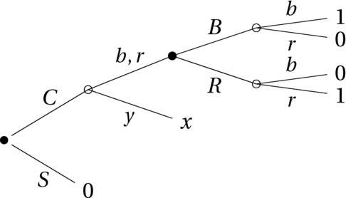
Figure 3. A dynamic version of the Ellsberg Paradox; x ∈{0, 1}.

Suppose that the urn contains 30 black balls, and no more than 30 red balls. The DM's prior MEU preferences are then characterized by the set C′ of probabilities P such that P(b)= and P(r) ≤ ; note that C′ contains the uniform prior on {b, r, y}, denoted P _u. The plan (C, R) is ex-ante optimal in the tree f ₁; to ensure dynamic consistency, the Hanany and Klibanoff ambiguity-maximizing rule requires that only the uniform prior P _u be updated upon reaching the second decision node; all other elements of C′ must be discarded. Therefore, the DM must have EU preferences upon learning that the ball drawn was not yellow in the tree f ₁. By way of contrast, the unique optimal plan in the tree f ₀ is (C, B), and the Hanany and Klibanoff ambiguity-maximizing rule prescribes that all priors in C′ be updated: thus, the DM has non-degenerate MEU preferences at the second decision node in the tree f ₀.Footnote ⁷ Hence, conditional upon {b, r}, the DM does not perceive ambiguity in f ₁, but does perceive it in f ₀, despite the fact that she receives the same information.

This conclusion stands in sharp contrast with the prevailing view in the literature, which emphasizes that ambiguity is an informational phenomenon. For instance, Ellsberg defines ambiguity as “a quality depending on the amount, type, reliability and ‘unanimity’ of the information” (Ellsberg Reference Ellsberg1961: 657).Footnote ⁸ If the non-consequentialist approach advocated by Hanany and Klibanoff is adopted, ambiguity must be allowed to depend upon the entire “context” of the (conditional) decision problem, including foregone payoffs and the ex-ante optimal plan that is to be carried out. This strikes me as a significant departure from our usual understanding of ambiguity, and a high price to pay in exchange for dynamic consistency.

One may object that the “information” the DM receives at the second decision node in Figure 3 includes the fact that she has avoided the payoff 0 in the tree f ₀, and foregone the payoff 1 in the tree f ₁. But doing so would broaden the interpretation of “information” much beyond its conventional meaning of “partial resolution of the uncertainty” (as evinced from expressions such as “information partition”). After all, there is no uncertainty about the payoff that might have been obtained if the ball drawn had been yellow.

I emphasize that the above arguments are specific to choice in the presence of ambiguity. They clearly do not apply to the setting of risky choice: if probabilities are “given”, ambiguity simply cannot arise. Second, even in the setting of choice under uncertainty, these arguments do not apply to non-EU preferences that are probabilistically sophisticated: in this case, by definition the DM does not perceive any ambiguity.