


1. Introduction
The principal motivation for the development of drag reducing techniques is the desire to reduce energy costs associated with transportation. The mechanisms responsible for drag generation can be conveniently categorized as those associated with the pressure form drag, the pressure interaction drag and the shear drag (Mohammadi & Floryan Reference Mohammadi and Floryan2012). The first mechanism and techniques for its reduction are well understood. The second mechanism is relevant for flows over surface topographies, and the understanding of this mechanism is limited. The third mechanism has a simple physical origin, but the development of techniques for its reduction represents a significant challenge. This reduction can be achieved either directly by rearranging the form of the flow or indirectly by delaying the laminar–turbulent transition. The desired change must come from altering the form of the fluid layer adjacent to the solid wall, and this can be accomplished by either passive or active means. The commonly explored techniques include changing the wall topography, applying suction/blowing or relying on plasma-, sound- or piezo-driven actuators.
This work is focused on the development of techniques for reduction of the laminar shear drag. It had been believed that reduction of this drag is not possible (Choi, Moin & Kim Reference Choi, Moin and Kim1991; Chu & Karniadakis Reference Chu and Karniadakis1993), as any changes in surface topography increase the wetted area exposed to friction, which must be more than balanced by the reduction of shear. At present there are three techniques that can achieve this goal. In the first one, the use of properly structured grooves leads to changes in the bulk flow which reduce the shear sufficiently to overcome the associated increase of surface area exposed to friction (Mohammadi & Floryan Reference Mohammadi and Floryan2013a ). The groove shapes can be optimized (Mohammadi & Floryan Reference Mohammadi and Floryan2013b ), with the optimal groove having a universal shape which depends on the constraints used. In the case of grooves with equal height and depth the universal shape has a trapezoidal form while in the case of grooves with different depth and height it has a Gaussian shape.
The second technique relies on the superhydrophobic effect (Rothstein Reference Rothstein2010). The surface topography traps gas bubbles in micropores and, thus, replaces the shear between the liquid stream and the solid wall with a shear between the stream and the gas in the bubbles. This effect is active in two-phase systems and its effectiveness depends on the hydrophobicity of the liquid and surface material and details of the surface topography. The effectiveness of this method can be increased by correctly shaping the surface pores (Samaha, Tafreshi & Gad-el-Hak Reference Samaha, Tafreshi and Gad-el-Hak2011) and by increasing hydrophobicity through changes in surface chemistry (Quéré Reference Quéré2008; Reyssat, Yeomans & Quéré Reference Reyssat, Yeomans and Quéré2008; Zhou et al. Reference Zhou, Li, Wu, Zhou and Cai2011). The occurrence of laminar drag reduction has been demonstrated by Ou, Perot & Rothstein (Reference Ou, Perot and Rothstein2004), Ou & Rothstein (Reference Ou and Rothstein2005), Joseph et al. (Reference Joseph, Cottin-Bizonne, Benoit, Ybert, Journet, Tabeling and Bocquet2006) and Truesdell et al. (Reference Truesdell, Mammoli, Vorobieff, van Swol and Brinker2006) among others. It is uncertain how the surface topography interacts with the pressure field, but experimental measurements demonstrate an overall drag reduction.
The third technique relies on spatially distributed heating; this creates a buoyancy field which, in turn, generates separation bubbles. The bubbles isolate the stream from direct contact with the bounding walls. Motion inside the bubbles is supported by the horizontal density gradients; these provide an additional propulsive force which reduces the required pressure gradient. This effect, sometimes referred to as the superthermohydrophobic effect (Floryan Reference Floryan2012), is active in single-phase fluids and is independent of surface topography. It remains effective for very small Reynolds numbers (Hossain, Floryan & Floryan Reference Hossain, Floryan and Floryan2012), since stronger flows wash the separation bubbles away, and, thus, it is relevant for applications in narrow conduits. The main objective of this analysis is to identify means for increasing the effectiveness of this effect by exploring different heating conditions. In particular, we focus our attention on the gains associated with the use of a combination of uniform and spatially modulated heating components. A model problem and the relevant formulation are discussed in § 2. The solution method is described in § 3. Properties of the long-wavelength heating are discussed in § 4. Characteristics of the short-wavelength heating are described in § 5. Heating with an arbitrary wavenumber is discussed in § 6 with detailed results presented for the Prandtl number
 $\mathit{Pr}=0.71$
, which well approximates the properties of air. In particular, the effects of the strength of the external stream are described in § 6.1, the effects of the heating conditions are presented in § 6.2 and the energy fluxes are discussed in § 6.3. Section 7 gives a short summary of the main conclusions.
$\mathit{Pr}=0.71$
, which well approximates the properties of air. In particular, the effects of the strength of the external stream are described in § 6.1, the effects of the heating conditions are presented in § 6.2 and the energy fluxes are discussed in § 6.3. Section 7 gives a short summary of the main conclusions.

Figure 1. Sketch of the system configuration.
2. Problem formulation
Consider steady two-dimensional flow of a fluid confined in a channel bounded by two parallel walls extending to
 $\pm \infty$
in the
$\pm \infty$
in the
 $x$
direction (horizontal direction) and placed a distance
$x$
direction (horizontal direction) and placed a distance
 $2h$
apart with the gravitational acceleration
$2h$
apart with the gravitational acceleration
 $g$
acting in the negative
$g$
acting in the negative
 $y$
direction (vertical direction), as shown in figure 1. The flow is driven in the positive
$y$
direction (vertical direction), as shown in figure 1. The flow is driven in the positive
 $x$
direction by a pressure gradient. The fluid is incompressible and Newtonian with thermal conductivity
$x$
direction by a pressure gradient. The fluid is incompressible and Newtonian with thermal conductivity
 $k$
, specific heat
$k$
, specific heat
 $c$
, thermal diffusivity
$c$
, thermal diffusivity
 ${\it\kappa}=k/{\it\rho}c$
, kinematic viscosity
${\it\kappa}=k/{\it\rho}c$
, kinematic viscosity
 ${\it\nu}$
, dynamic viscosity
${\it\nu}$
, dynamic viscosity
 ${\it\mu}$
, thermal expansion coefficient
${\it\mu}$
, thermal expansion coefficient
 ${\it\Gamma}$
and variations of the density
${\it\Gamma}$
and variations of the density
 ${\it\rho}$
that follow the Boussinesq approximation. The flow is modified by subjecting the lower wall to a spatially distributed heating, resulting in wall temperatures of the form
${\it\rho}$
that follow the Boussinesq approximation. The flow is modified by subjecting the lower wall to a spatially distributed heating, resulting in wall temperatures of the form
 $$\begin{eqnarray}{\it\theta}_{L}(x)=\mathop{\sum }_{n=-\infty }^{n=+\infty }{\it\theta}_{L}^{(n)}\text{e}^{\text{i}n{\it\alpha}x},\quad {\it\theta}_{U}(x)=0,\end{eqnarray}$$
where
 ${\it\theta}$
denotes the difference between the actual temperature and the temperature of the upper wall,
${\it\theta}$
denotes the difference between the actual temperature and the temperature of the upper wall,
 ${\it\theta}=T-T_{U}$
,
${\it\theta}=T-T_{U}$
,
 $T$
denotes the absolute temperature,
$T$
denotes the absolute temperature,
 ${\it\theta}_{L}^{(n)}={\it\theta}_{L}^{(-n)\ast }$
are the reality conditions, stars denote complex conjugates,
${\it\theta}_{L}^{(n)}={\it\theta}_{L}^{(-n)\ast }$
are the reality conditions, stars denote complex conjugates,
 ${\it\lambda}=2{\rm\pi}/{\it\alpha}$
is the wavelength of the heating,
${\it\lambda}=2{\rm\pi}/{\it\alpha}$
is the wavelength of the heating,
 ${\it\alpha}$
is its wavenumber and the subscripts
${\it\alpha}$
is its wavenumber and the subscripts
 $L$
and
$L$
and
 $U$
refer to the lower and upper walls respectively. The heating can be divided into the uniform heating described by
$U$
refer to the lower and upper walls respectively. The heating can be divided into the uniform heating described by
 ${\it\theta}_{L}^{(0)}$
and the spatially modulated heating described by the remaining terms in (2.1a
). The conductive temperature field
${\it\theta}_{L}^{(0)}$
and the spatially modulated heating described by the remaining terms in (2.1a
). The conductive temperature field
 ${\it\theta}_{0}$
corresponding to the above heating is, in the absence of any fluid movement, described by
${\it\theta}_{0}$
corresponding to the above heating is, in the absence of any fluid movement, described by
 $$\begin{eqnarray}\frac{\partial ^{2}{\it\theta}_{0}}{\partial x^{2}}+\frac{\partial ^{2}{\it\theta}_{0}}{\partial y^{2}}=0,\end{eqnarray}$$
subject to the boundary conditions (2.1). The solution has the form
 $$\begin{eqnarray}{\it\theta}_{0}(x,y)=\frac{\mathit{Ra}_{uni}}{\mathit{Ra}_{per}}\hat{{\it\theta}}_{0}(y)+\hat{\hat{{\it\theta}}}_{0}(x,y),\end{eqnarray}$$
where
 $$\begin{eqnarray}\displaystyle \hat{{\it\theta}}_{0}(y)={\textstyle \frac{1}{2}}(1-y),\end{eqnarray}$$
 $$\begin{eqnarray}\displaystyle & \displaystyle \hat{\hat{{\it\theta}}}_{0}(x,y)=\mathop{\sum }_{n=-\infty ,n\neq 0}^{n=+\infty }\hat{\hat{{\it\theta}}}_{0}^{(n)}(y)\text{e}^{\text{i}n{\it\alpha}x}=\mathop{\sum }_{n=-\infty ,n\neq 0}^{n=+\infty }\left\{\frac{1}{2}{\it\theta}_{L}^{(n)}\left[\frac{\cosh (n{\it\alpha}y)}{\cosh (n{\it\alpha})}-\frac{\sinh (n{\it\alpha}y)}{\sinh (n{\it\alpha})}\right]\right\}\text{e}^{\text{i}n{\it\alpha}x} & \displaystyle \nonumber\\ \displaystyle & & \displaystyle\end{eqnarray}$$
and
 $\hat{\hat{{\it\theta}}}_{0}^{(n)}=\hat{\hat{{\it\theta}}}_{0}^{(-n)^{\ast }}$
are the reality conditions. The uniform temperature component
$\hat{\hat{{\it\theta}}}_{0}^{(n)}=\hat{\hat{{\it\theta}}}_{0}^{(-n)^{\ast }}$
are the reality conditions. The uniform temperature component
 $\hat{{\it\theta}}_{0}$
has been scaled with the difference
$\hat{{\it\theta}}_{0}$
has been scaled with the difference
 $T_{uni}$
between the mean temperature of the lower wall and the temperature of the upper wall, and the complete temperature
$T_{uni}$
between the mean temperature of the lower wall and the temperature of the upper wall, and the complete temperature
 ${\it\theta}_{0}$
, as well as its spatially modulated part, has been scaled with a conveniently selected temperature scale
${\it\theta}_{0}$
, as well as its spatially modulated part, has been scaled with a conveniently selected temperature scale
 $T_{per}$
characterizing the amplitude of the spatial modulations. The channel half-height
$T_{per}$
characterizing the amplitude of the spatial modulations. The channel half-height
 $h$
has been used as the length scale. The Rayleigh numbers based on the uniform and spatial modulation temperature scales are defined as
$h$
has been used as the length scale. The Rayleigh numbers based on the uniform and spatial modulation temperature scales are defined as
 $\mathit{Ra}_{uni}=g{\it\Gamma}h^{3}T_{uni}/{\it\nu}{\it\kappa}$
and
$\mathit{Ra}_{uni}=g{\it\Gamma}h^{3}T_{uni}/{\it\nu}{\it\kappa}$
and
 $\mathit{Ra}_{per}=g{\it\Gamma}h^{3}T_{per}/{\it\nu}{\it\kappa}$
respectively. When the spatial modulation of the heating is limited to just one Fourier mode of the form
$\mathit{Ra}_{per}=g{\it\Gamma}h^{3}T_{per}/{\it\nu}{\it\kappa}$
respectively. When the spatial modulation of the heating is limited to just one Fourier mode of the form
 ${\it\theta}_{L}(x)=\cos ({\it\alpha}x)/2$
, (2.3c
) simplifies to the form
${\it\theta}_{L}(x)=\cos ({\it\alpha}x)/2$
, (2.3c
) simplifies to the form
 $$\begin{eqnarray}\hat{\hat{{\it\theta}}}_{0}(x,y)=\hat{\hat{{\it\theta}}}_{0}^{(1)}(y)\text{e}^{\text{i}{\it\alpha}x}+\text{c.c.}=\frac{1}{8}\left[\frac{\cosh ({\it\alpha}y)}{\cosh ({\it\alpha})}-\frac{\sinh ({\it\alpha}y)}{\sinh ({\it\alpha})}\right]\text{e}^{\text{i}n{\it\alpha}x}+\text{c.c.},\end{eqnarray}$$
and the amplitude of the temperature variations along the lower wall serves as the temperature scale
 $T_{per}$
. In the above, c.c. stands for the complex conjugate.
$T_{per}$
. In the above, c.c. stands for the complex conjugate.
The velocity and pressure fields in the absence of the heating have the form
 $$\begin{eqnarray}\boldsymbol{v}_{0}(x,y)=[u_{0}(y),0]=[1-y^{2},0],\quad p_{0}(x,y)=-2x/\mathit{Re},\end{eqnarray}$$
where
 $\boldsymbol{v}_{0}=(u_{0},v_{0})$
denotes the velocity vector scaled with the maximum of the
$\boldsymbol{v}_{0}=(u_{0},v_{0})$
denotes the velocity vector scaled with the maximum of the
 $x$
-velocity
$x$
-velocity
 $U_{max}$
,
$U_{max}$
,
 $p_{0}$
stands for the pressure scaled with
$p_{0}$
stands for the pressure scaled with
 ${\it\rho}U_{max}^{2}$
and the Reynolds number is defined as
${\it\rho}U_{max}^{2}$
and the Reynolds number is defined as
 $\mathit{Re}=U_{max}h/{\it\nu}$
.
$\mathit{Re}=U_{max}h/{\it\nu}$
.
The heating produces convection, and the resulting changes in the flow and temperature fields can be represented as
 $$\begin{eqnarray}\left.\begin{array}{@{}c@{}}u_{T}(x,y)=\mathit{Re}u_{0}(y)+u_{1}(x,y),\quad v_{T}(x,y)=v_{1}(x,y),\\ {\it\theta}_{T}(x,y)=\mathit{Pr}^{-1}{\it\theta}_{0}(x,y)+{\it\theta}_{1}(x,y),\quad p_{T}(x,y)=\mathit{Re}^{2}p_{0}(x)+p_{1}(x,y).\end{array}\right\}\end{eqnarray}$$
In the above,
 $(u_{T},v_{T}),p_{T}$
and
$(u_{T},v_{T}),p_{T}$
and
 ${\it\theta}_{T}$
denote the complete velocity, pressure and temperature fields respectively and
${\it\theta}_{T}$
denote the complete velocity, pressure and temperature fields respectively and
 $(u_{1},v_{1})$
,
$(u_{1},v_{1})$
,
 $p_{1}$
and
$p_{1}$
and
 ${\it\theta}_{1}$
denote the velocity, pressure and temperature field modifications caused by the heating respectively. The complete velocity vector and the velocity modifications have been scaled using the convective velocity scale
${\it\theta}_{1}$
denote the velocity, pressure and temperature field modifications caused by the heating respectively. The complete velocity vector and the velocity modifications have been scaled using the convective velocity scale
 $U_{v}={\it\nu}/h$
, where
$U_{v}={\it\nu}/h$
, where
 $U_{max}/U_{v}=\mathit{Re}$
, the pressure modifications have been scaled using
$U_{max}/U_{v}=\mathit{Re}$
, the pressure modifications have been scaled using
 ${\it\rho}U_{v}^{2}$
and the total and convective temperatures have been scaled using the convective temperature scale
${\it\rho}U_{v}^{2}$
and the total and convective temperatures have been scaled using the convective temperature scale
 $T_{v}$
, where
$T_{v}$
, where
 $T_{v}/T_{per}=\mathit{Pr}$
, with
$T_{v}/T_{per}=\mathit{Pr}$
, with
 $\mathit{Pr}$
denoting the Prandtl number. The field equations for the flow and temperature modifications have the form
$\mathit{Pr}$
denoting the Prandtl number. The field equations for the flow and temperature modifications have the form
 $$\begin{eqnarray}\displaystyle & \displaystyle (\mathit{Re}u_{0}+u_{1})\frac{\partial u_{1}}{\partial x}+\mathit{Re}v_{1}\frac{\text{d}u_{0}}{\text{d}y}+v_{1}\frac{\partial u_{1}}{\partial y}=-\frac{\partial p_{1}}{\partial x}+\frac{\partial ^{2}u_{1}}{\partial x^{2}}+\frac{\partial ^{2}u_{1}}{\partial y^{2}}, & \displaystyle\end{eqnarray}$$
 $$\begin{eqnarray}\displaystyle & \displaystyle (\mathit{Re}u_{0}+u_{1})\frac{\partial v_{1}}{\partial x}+v_{1}\frac{\partial v_{1}}{\partial y}=-\frac{\partial p_{1}}{\partial y}+\frac{\partial ^{2}v_{1}}{\partial x^{2}}+\frac{\partial ^{2}v_{1}}{\partial y^{2}}+\mathit{Ra}_{per}{\it\theta}_{1} & \displaystyle \nonumber\\ \displaystyle & \displaystyle \hspace{108.0pt}\quad +\,\mathit{Ra}_{uni}\mathit{Pr}^{-1}\hat{{\it\theta}}_{0}+\mathit{Ra}_{per}\mathit{Pr}^{-1}\hat{\hat{{\it\theta}}}_{0}, & \displaystyle\end{eqnarray}$$
 $$\begin{eqnarray}\displaystyle & \displaystyle (\mathit{Re}u_{0}+u_{1})\left(\frac{\partial \hat{\hat{{\it\theta}}}_{0}}{\partial x}+\mathit{Pr}\frac{\partial {\it\theta}_{1}}{\partial x}\right)+v_{1}\left(-\frac{\mathit{Ra}_{uni}}{2\mathit{Ra}_{per}}+\frac{\partial \hat{\hat{{\it\theta}}}_{0}}{\partial y}+\mathit{Pr}\frac{\partial {\it\theta}_{1}}{\partial y}\right)=\frac{\partial ^{2}{\it\theta}_{1}}{\partial x^{2}}+\frac{\partial ^{2}{\it\theta}_{1}}{\partial y^{2}}, & \displaystyle \nonumber\\ \displaystyle & & \displaystyle\end{eqnarray}$$
 $$\begin{eqnarray}\displaystyle & \displaystyle \frac{\partial u_{1}}{\partial x}+\frac{\partial v_{1}}{\partial y}=0. & \displaystyle\end{eqnarray}$$
The main goal of the analysis is the determination of the mean pressure modification
 $p_{1}$
, as it provides information about the ability of the heating to change the flow pressure losses. The physical problem of the determination of pressure losses is posed as the question of finding the additional pressure gradient that is required in order to maintain the same flow rate in the heated and isothermal channels. The equality of flow rates is imposed through the flow rate constraint of the form
$p_{1}$
, as it provides information about the ability of the heating to change the flow pressure losses. The physical problem of the determination of pressure losses is posed as the question of finding the additional pressure gradient that is required in order to maintain the same flow rate in the heated and isothermal channels. The equality of flow rates is imposed through the flow rate constraint of the form
 $$\begin{eqnarray}Q=\int _{-1}^{1}u_{T}\text{d}y=\int _{-1}^{1}(\mathit{Re}u_{0}+u_{1})\text{d}y=4\mathit{Re}/3.\end{eqnarray}$$
Elimination of the imposed flow corresponds to the limit
 $\mathit{Re}\rightarrow 0$
. Elimination of the heating results in
$\mathit{Re}\rightarrow 0$
. Elimination of the heating results in
 $u_{1}=v_{1}=p_{1}={\it\theta}_{1}=0$
, with the flow field being described by (2.2). This corresponds to the limit
$u_{1}=v_{1}=p_{1}={\it\theta}_{1}=0$
, with the flow field being described by (2.2). This corresponds to the limit
 $\mathit{Ra}_{per}\rightarrow 0$
, although the temperature scaling would have to be adjusted in order to avoid an artificial singularity in (2.3a
). It is assumed in the further analysis that
$\mathit{Ra}_{per}\rightarrow 0$
, although the temperature scaling would have to be adjusted in order to avoid an artificial singularity in (2.3a
). It is assumed in the further analysis that
 $\mathit{Ra}_{per}$
is never zero, as the primary effect leading to drag reduction is associated with spatial temperature variations.
$\mathit{Ra}_{per}$
is never zero, as the primary effect leading to drag reduction is associated with spatial temperature variations.
Selection of system parameters suitable for the analysis requires care due to the ease with which secondary flows can be induced. In general, such flows are expected to increase pressure losses and, thus, should be avoided. It has been found in this analysis that this is not always the case; under some conditions systems with secondary flows produced greater drag reduction than systems without secondary flows. An increase of
 $\mathit{Re}$
increases the mixed convection and this could, eventually, lead to shear-driven instabilities; the
$\mathit{Re}$
increases the mixed convection and this could, eventually, lead to shear-driven instabilities; the
 $\mathit{Re}$
values of interest in this analysis are small enough that such instabilities do not occur (Orszag Reference Orszag1971). The uniform heating could lead to a secondary flow through buoyancy-driven instability (Rayleigh–Bénard or RB mechanism; Chandrasekhar (Reference Chandrasekhar1961)); the critical value of
$\mathit{Re}$
values of interest in this analysis are small enough that such instabilities do not occur (Orszag Reference Orszag1971). The uniform heating could lead to a secondary flow through buoyancy-driven instability (Rayleigh–Bénard or RB mechanism; Chandrasekhar (Reference Chandrasekhar1961)); the critical value of
 $\mathit{Ra}_{uni}$
required for the onset of such convection in the absence of both forced flow and periodic heating is
$\mathit{Ra}_{uni}$
required for the onset of such convection in the absence of both forced flow and periodic heating is
 $\mathit{Ra}_{uni}=213.5$
. Freund, Pesch & Zimmermann (Reference Freund, Pesch and Zimmermann2011) have demonstrated that the addition of a small-amplitude periodic heating generally decreases the
$\mathit{Ra}_{uni}=213.5$
. Freund, Pesch & Zimmermann (Reference Freund, Pesch and Zimmermann2011) have demonstrated that the addition of a small-amplitude periodic heating generally decreases the
 $\mathit{Ra}_{uni}$
required for the onset. Larger values of
$\mathit{Ra}_{uni}$
required for the onset. Larger values of
 $\mathit{Ra}_{per}$
are expected to activate the spatial parametric resonance in addition to the RB mechanism, but such a situation is yet to be studied. Hossain & Floryan (Reference Hossain and Floryan2013) demonstrated that the spatially periodic heating can, by itself, lead to an instability, which is driven either by the RB mechanism or by the spatial parametric resonance. The addition of a forced flow and removal of the spatially modulated heating maintains the same critical conditions as for the uniform heating, i.e.
$\mathit{Ra}_{per}$
are expected to activate the spatial parametric resonance in addition to the RB mechanism, but such a situation is yet to be studied. Hossain & Floryan (Reference Hossain and Floryan2013) demonstrated that the spatially periodic heating can, by itself, lead to an instability, which is driven either by the RB mechanism or by the spatial parametric resonance. The addition of a forced flow and removal of the spatially modulated heating maintains the same critical conditions as for the uniform heating, i.e.
 $\mathit{Ra}_{uni}=213.5$
(Gage & Reid Reference Gage and Reid1968). The conditions leading to the onset of secondary flows when all these effects are present have yet to be determined. The small magnitudes of
$\mathit{Ra}_{uni}=213.5$
(Gage & Reid Reference Gage and Reid1968). The conditions leading to the onset of secondary flows when all these effects are present have yet to be determined. The small magnitudes of
 $\mathit{Ra}_{per}$
and
$\mathit{Ra}_{per}$
and
 $\mathit{Ra}_{uni}$
considered in this analysis minimize the potential for the formation of secondary flows. Since the conditions leading to the onset are yet to be determined, extreme care needs to be exercised when interpreting the results.
$\mathit{Ra}_{uni}$
considered in this analysis minimize the potential for the formation of secondary flows. Since the conditions leading to the onset are yet to be determined, extreme care needs to be exercised when interpreting the results.
The problem formulation is closed by specifying the no-slip, no-penetration and thermal boundary conditions at the bounding walls, which have the form
 $$\begin{eqnarray}u_{1}(\pm 1)=0,\quad v_{1}(\pm 1)=0,\quad {\it\theta}_{1}(\pm 1)=0.\end{eqnarray}$$
The solution of (2.6)–(2.8) results in the determination of the velocity, temperature and pressure fields, including the mean pressure gradient, which is the main interest.
3. Method of solution
We define the stream function
 ${\it\psi}(x,y)$
in the usual manner, i.e.
${\it\psi}(x,y)$
in the usual manner, i.e.
 $u_{1}=\partial {\it\psi}/\partial y$
,
$u_{1}=\partial {\it\psi}/\partial y$
,
 $v_{1}=-\partial {\it\psi}/\partial x$
, and assume the solution to be of the form
$v_{1}=-\partial {\it\psi}/\partial x$
, and assume the solution to be of the form
 $$\begin{eqnarray}{\it\psi}(x,y)=\mathop{\sum }_{n=-\infty }^{n=+\infty }{\it\varphi}^{(n)}(y)\text{e}^{\text{i}n{\it\alpha}x},\quad {\it\theta}_{1}(x,y)=\mathop{\sum }_{n=-\infty }^{n=+\infty }{\it\phi}^{(n)}(y)\text{e}^{\text{i}n{\it\alpha}x},\end{eqnarray}$$
where
 ${\it\varphi}^{(n)}={\it\varphi}^{(-n)\ast }$
and
${\it\varphi}^{(n)}={\it\varphi}^{(-n)\ast }$
and
 ${\it\phi}^{(n)}={\it\phi}^{(-n)\ast }$
are the reality conditions. Substitution of (3.1) into the field equations, elimination of pressure and separation of Fourier components result in the following system of ordinary differential equations for the modal functions:
${\it\phi}^{(n)}={\it\phi}^{(-n)\ast }$
are the reality conditions. Substitution of (3.1) into the field equations, elimination of pressure and separation of Fourier components result in the following system of ordinary differential equations for the modal functions:
 $$\begin{eqnarray}\displaystyle & & \displaystyle \text{D}_{n}^{2}{\it\varphi}^{(n)}-\text{i}n{\it\alpha}\mathit{Re}(u_{0}\text{D}_{n}-\text{D}^{2}u_{0}){\it\varphi}^{(n)}-\text{i}n{\it\alpha}\mathit{Ra}_{per}{\it\phi}^{(n)}-\text{i}n{\it\alpha}\mathit{Ra}_{per}\mathit{Pr}^{-1}\hat{\hat{{\it\theta}}}_{0}^{(n)}\nonumber\\ \displaystyle & & \displaystyle \quad -\,\text{i}{\it\alpha}\mathop{\sum }_{m=-\infty }^{m=+\infty }[\text{D}{\it\varphi}^{(n-m)}m\text{D}_{m}{\it\varphi}^{(m)}-(n-m){\it\varphi}^{(n-m)}\text{D}_{m}(\text{D}{\it\varphi}^{(m)})]=0,\end{eqnarray}$$
 $$\begin{eqnarray}\displaystyle & & \displaystyle \text{D}_{n}{\it\phi}^{(n)}-\text{i}n{\it\alpha}\mathit{Pr}\mathit{Re}u_{0}{\it\phi}^{(n)}-\text{i}n{\it\alpha}\mathit{Re}u_{0}\hat{\hat{{\it\theta}}}_{0}^{(n)}-\text{i}n{\it\alpha}\frac{\mathit{Ra}_{uni}}{2\mathit{Ra}_{per}}{\it\varphi}^{(n)}\nonumber\\ \displaystyle & & \displaystyle \quad -\,\mathop{\sum }_{m=-\infty }^{m=+\infty }\left[\text{i}{\it\alpha}(n-m)(\hat{\hat{{\it\theta}}}_{0}^{(n-m)}+\mathit{Pr}{\it\phi}^{(n-m)})\text{D}{\it\varphi}^{(m)}\right.\nonumber\\ \displaystyle & & \displaystyle \left.\quad -\,\text{i}m{\it\alpha}{\it\varphi}^{(m)}\text{D}(\hat{\hat{{\it\theta}}}_{0}^{(n-m)}+\mathit{Pr}{\it\phi}^{(n-m)})\right]=0,\end{eqnarray}$$
 $\text{D}=\text{d}/\text{d}y$
,
$\text{D}=\text{d}/\text{d}y$
,
 $\text{D}_{n}=\text{D}^{2}-n^{2}{\it\alpha}^{2}$
,
$\text{D}_{n}=\text{D}^{2}-n^{2}{\it\alpha}^{2}$
,
 $\text{D}_{n}^{2}=\text{D}^{4}-2n^{2}{\it\alpha}^{2}\text{D}^{2}+n^{4}{\it\alpha}^{4}$
,
$\text{D}_{n}^{2}=\text{D}^{4}-2n^{2}{\it\alpha}^{2}\text{D}^{2}+n^{4}{\it\alpha}^{4}$
,
 $-\infty <n<+\infty$
. The relevant boundary conditions have the form
$-\infty <n<+\infty$
. The relevant boundary conditions have the form  $$\begin{eqnarray}\text{D}{\it\varphi}^{(n)}(\pm 1)=0,\quad {\it\varphi}^{(n)}(\pm 1)=0,\quad {\it\phi}^{(n)}(\pm 1)=0,\end{eqnarray}$$
and account for the flow rate constraint.
Expansions (3.1) are truncated after a finite number of terms
 $N_{M}$
, resulting in a system of
$N_{M}$
, resulting in a system of
 $2(2N_{M}+1)$
equations of type (3.2) and (3.3) which are solved using the variable-step-size finite-difference discretization based on the Simpson method with deferred corrections (Kierzenka & Shampine Reference Kierzenka and Shampine2001, Reference Kierzenka and Shampine2008). The resulting algebraic system is solved using a simplified Newton (chord) method with residual control. Selection of the number and distribution of the grid points is carried out automatically to meet the specified error bounds. The number of Fourier modes used in the solution has been selected through numerical experiments to guarantee at least six digits accuracy.
$2(2N_{M}+1)$
equations of type (3.2) and (3.3) which are solved using the variable-step-size finite-difference discretization based on the Simpson method with deferred corrections (Kierzenka & Shampine Reference Kierzenka and Shampine2001, Reference Kierzenka and Shampine2008). The resulting algebraic system is solved using a simplified Newton (chord) method with residual control. Selection of the number and distribution of the grid points is carried out automatically to meet the specified error bounds. The number of Fourier modes used in the solution has been selected through numerical experiments to guarantee at least six digits accuracy.
In the postprocessing stage, the velocity field is evaluated according to the relations
 $$\begin{eqnarray}\displaystyle u_{1}(x,y)=\mathop{\sum }_{n=-\infty }^{n=+\infty }u_{1}^{(n)}(y)\text{e}^{\text{i}n{\it\alpha}x}=\mathop{\sum }_{n=-\infty }^{n=+\infty }\text{D}{\it\varphi}^{(n)}(y)\text{e}^{\text{i}n{\it\alpha}x}, & & \displaystyle\end{eqnarray}$$
 $$\begin{eqnarray}\displaystyle v_{1}(x,y)=\mathop{\sum }_{n=-\infty }^{n=+\infty }v_{1}^{(n)}(y)\text{e}^{\text{i}n{\it\alpha}x}=-\mathop{\sum }_{n=-\infty }^{n=+\infty }\text{i}{\it\alpha}{\it\varphi}^{(n)}(y)\text{e}^{\text{i}n{\it\alpha}x}. & & \displaystyle\end{eqnarray}$$
 $$\begin{eqnarray}p_{1}(x,y)=Ax+\mathop{\sum }_{n=-\infty }^{n=+\infty }p_{1}^{(n)}(y)\text{e}^{\text{i}n{\it\alpha}x},\end{eqnarray}$$
where
 $A$
represents the pressure gradient change induced by the heating, and positive values correspond to drag reduction. The pressure gradient correction
$A$
represents the pressure gradient change induced by the heating, and positive values correspond to drag reduction. The pressure gradient correction
 $A$
can be computed on the basis of (3.2) written for mode zero, which can be brought to the following form
$A$
can be computed on the basis of (3.2) written for mode zero, which can be brought to the following form
 $$\begin{eqnarray}\text{D}^{4}{\it\varphi}^{(0)}=\mathop{\sum }_{n=-\infty }^{n=+\infty }\text{D}^{2}(\text{i}n{\it\alpha}{\it\varphi}^{(-n)}\text{D}{\it\varphi}^{(n)}).\end{eqnarray}$$
Double integration and application of the boundary conditions yield an explicit relation for
 $A$
of the form
$A$
of the form
 $$\begin{eqnarray}A={\textstyle \frac{1}{2}}[\text{D}^{2}{\it\varphi}^{(0)}(1)-\text{D}^{2}{\it\varphi}^{(0)}(-1)],\end{eqnarray}$$
which can be readily evaluated. Another method can be derived by substituting (3.5) and (3.6) into (2.6a ) and extracting mode zero to arrive at
 $$\begin{eqnarray}\text{D}^{2}u_{1}^{(0)}=\text{D}g+A,\end{eqnarray}$$
where
 $$\begin{eqnarray}g(y)=\mathop{\sum }_{n=-\infty }^{n=+\infty }v_{1}^{(-n)}u_{1}^{(n)}.\end{eqnarray}$$
Double integration and use of the boundary conditions and the flow rate constraint lead to
 $$\begin{eqnarray}A={\textstyle \frac{3}{2}}(K_{1}-K_{2}),\end{eqnarray}$$
where
 $$\begin{eqnarray}K_{1}=\int _{-1}^{1}f(y)\text{d}y,\quad K_{2}=\int _{-1}^{1}g(y)\text{d}y,\quad f(y)=\int _{-1}^{y}g({\it\eta})\text{d}{\it\eta}.\end{eqnarray}$$
In the above,
 $g(y)$
is referred to as the Reynolds stress function resulting from the integration of this stress over one wavelength in the
$g(y)$
is referred to as the Reynolds stress function resulting from the integration of this stress over one wavelength in the
 $x$
direction,
$x$
direction,
 $K_{2}$
represents the result of the subsequent integration across the channel and
$K_{2}$
represents the result of the subsequent integration across the channel and
 $K_{1}$
results from the repetition of the same integration process. Equation (3.10) demonstrates that changes in the pressure gradient are associated with the Reynolds stress field created by the natural convection and modified by the stream forced to flow through the channel. Here,
$K_{1}$
results from the repetition of the same integration process. Equation (3.10) demonstrates that changes in the pressure gradient are associated with the Reynolds stress field created by the natural convection and modified by the stream forced to flow through the channel. Here,
 $A=0$
if the phase difference between
$A=0$
if the phase difference between
 $v_{1}^{(n)}$
and
$v_{1}^{(n)}$
and
 $u_{1}^{(n)}$
is
$u_{1}^{(n)}$
is
 ${\rm\pi}/2$
. The maximum of
${\rm\pi}/2$
. The maximum of
 $A$
is reached when
$A$
is reached when
 $v_{1}^{(n)}$
and
$v_{1}^{(n)}$
and
 $u_{1}^{(n)}$
are in phase. When
$u_{1}^{(n)}$
are in phase. When
 $\mathit{Re}=0$
, analysis of (3.2) and (3.3) demonstrates that
$\mathit{Re}=0$
, analysis of (3.2) and (3.3) demonstrates that
 ${\it\varphi}^{(n)}$
is imaginary,
${\it\varphi}^{(n)}$
is imaginary,
 ${\it\phi}^{(n)}$
is real,
${\it\phi}^{(n)}$
is real,
 $u_{1}^{(n)}$
is imaginary,
$u_{1}^{(n)}$
is imaginary,
 $v_{1}^{(n)}$
is real and, thus,
$v_{1}^{(n)}$
is real and, thus,
 $A=0$
. A non-zero value of
$A=0$
. A non-zero value of
 $\mathit{Re}$
is essential for the creation of the phase difference, i.e. the modifications of the Reynolds stress field by the external stream are essential for the creation of a non-zero
$\mathit{Re}$
is essential for the creation of the phase difference, i.e. the modifications of the Reynolds stress field by the external stream are essential for the creation of a non-zero
 $A$
. Elimination of the spatially modulated part of the heating (
$A$
. Elimination of the spatially modulated part of the heating (
 $\mathit{Ra}_{per}\rightarrow 0$
) eliminates
$\mathit{Ra}_{per}\rightarrow 0$
) eliminates
 $v_{1}^{(n)}$
and
$v_{1}^{(n)}$
and
 $u_{1}^{(n)}$
and, thus, eliminates any change in the pressure gradient. In the analysis, the pressure gradient correction has been computed using both (3.8) and (3.11) as part of the verification of the accuracy of the numerical solution.
$u_{1}^{(n)}$
and, thus, eliminates any change in the pressure gradient. In the analysis, the pressure gradient correction has been computed using both (3.8) and (3.11) as part of the verification of the accuracy of the numerical solution.
The total mean pressure gradient is represented as
 $$\begin{eqnarray}\left.\frac{\partial p_{T}}{\partial x}\right|_{mean}=\mathit{Re}(-2+A/\mathit{Re}),\end{eqnarray}$$
and the effectiveness of the heating can be judged by comparing
 $A/\mathit{Re}$
with
$A/\mathit{Re}$
with
 $-2$
.
$-2$
.
It is useful to close this section with relations that permit evaluation of the pressure modal functions. Relations obtained from the
 $x$
-momentum equation have the form
$x$
-momentum equation have the form
 $$\begin{eqnarray}\displaystyle p_{1}^{(n)} & = & \displaystyle \mathit{Re}u_{0}u_{1}^{(n)}-\frac{\text{i}}{n{\it\alpha}}\mathit{Re}\text{D}u_{0}v_{1}^{(n)}-\text{i}n{\it\alpha}u_{1}^{(n)}+\frac{\text{i}}{n{\it\alpha}}\text{D}^{2}u_{1}^{(n)}\nonumber\\ \displaystyle & & \displaystyle +\,\mathop{\sum }_{m=-\infty }^{m=+\infty }\left(\frac{n-m}{n}u_{1}^{(m)}u_{1}^{(n-m)}-\frac{\text{i}}{n{\it\alpha}}\text{D}u_{1}^{(m)}v_{1}^{(n-m)}\right),\quad n\neq 0.\end{eqnarray}$$
The relation for
 $p_{1}^{(0)}$
comes from the
$p_{1}^{(0)}$
comes from the
 $y$
-momentum equation and has the form
$y$
-momentum equation and has the form
 $$\begin{eqnarray}p_{1}^{(0)}=-\mathop{\sum }_{n=-\infty }^{n=+\infty }|v_{1}^{(n)}|^{2}+\mathit{Ra}_{per}\int {\it\phi}^{(0)}\text{d}y+\frac{\mathit{Ra}_{uni}}{\mathit{Pr}}\frac{y}{2}\left(1-\frac{y}{2}\right)+\text{const}.\end{eqnarray}$$
4. Long-wavelength heating (
 ${\it\alpha}\rightarrow 0$
)
${\it\alpha}\rightarrow 0$
)

We begin assessing the importance of the uniform heating by focusing our attention on a situation where the complete heating consists of a combination of uniform heating and spatially modulated heating whose distribution is described by just one Fourier component, e.g. (2.3d
). Because of the large number of parameters, we shall use asymptotic methods to identify the parameter ranges where a meaningful drag reduction can be achieved. We start this process by considering the long-wavelength limit of the spatially modulated heating, i.e.
 ${\it\alpha}\rightarrow 0$
. In the limit the periodic part of the conductive temperature field can be approximated as
${\it\alpha}\rightarrow 0$
. In the limit the periodic part of the conductive temperature field can be approximated as
 $$\begin{eqnarray}\hat{\hat{{\it\theta}}}_{0}(x,y)=\left[\hat{\hat{{\it\theta}}}_{00}(y)+{\it\alpha}^{2}\hat{\hat{{\it\theta}}}_{02}(y)+{\it\alpha}^{4}\hat{\hat{{\it\theta}}}_{04}(y)+0({\it\alpha}^{6})\right]\cos X,\end{eqnarray}$$
where definitions of
 $\hat{\hat{{\it\theta}}}_{00},\hat{\hat{{\it\theta}}}_{02},\hat{\hat{{\it\theta}}}_{04}$
are given in appendix A and
$\hat{\hat{{\it\theta}}}_{00},\hat{\hat{{\it\theta}}}_{02},\hat{\hat{{\it\theta}}}_{04}$
are given in appendix A and
 $X={\it\alpha}x$
denotes the slow scale. The field equations with
$X={\it\alpha}x$
denotes the slow scale. The field equations with
 $x$
replaced by the slow scale and with the uniform heating component taken out of the
$x$
replaced by the slow scale and with the uniform heating component taken out of the
 $y$
-momentum equation (see § 2) assume the form
$y$
-momentum equation (see § 2) assume the form
 $$\begin{eqnarray}\displaystyle & \displaystyle {\it\alpha}(\mathit{Re}u_{0}+u_{1})\frac{\partial u_{1}}{\partial X}+\mathit{Re}v_{1}\frac{\text{d}u_{0}}{\text{d}y}+v_{1}\frac{\partial u_{1}}{\partial y}=-{\it\alpha}\frac{\partial p_{1}}{\partial X}+{\it\alpha}^{2}\frac{\partial ^{2}u_{1}}{\partial X^{2}}+\frac{\partial ^{2}u_{1}}{\partial y^{2}},\qquad & \displaystyle\end{eqnarray}$$
 $$\begin{eqnarray}\displaystyle & \displaystyle {\it\alpha}(\mathit{Re}u_{0}+u_{1})\frac{\partial v_{1}}{\partial X}+v_{1}\frac{\partial v_{1}}{\partial y}=-\frac{\partial p_{1}}{\partial y}+{\it\alpha}^{2}\frac{\partial ^{2}v_{1}}{\partial X^{2}}+\frac{\partial ^{2}v_{1}}{\partial y^{2}}+\mathit{Ra}_{per}{\it\theta}_{1}+\mathit{Ra}_{per}\mathit{Pr}^{-1}\hat{\hat{{\it\theta}}}_{0}, & \displaystyle \nonumber\\ \displaystyle & & \displaystyle\end{eqnarray}$$
 $$\begin{eqnarray}\displaystyle & \displaystyle (\mathit{Re}u_{0}+u_{1})\left({\it\alpha}\frac{\partial \hat{\hat{{\it\theta}}}_{0}}{\partial X}+\mathit{Pr}{\it\alpha}\frac{\partial {\it\theta}_{1}}{\partial X}\right)+v_{1}\!\!\left(\!\!-\frac{\mathit{Ra}_{uni}}{2\mathit{Ra}_{per}}+\frac{\partial \hat{\hat{{\it\theta}}}_{0}}{\partial y}+\mathit{Pr}\frac{\partial {\it\theta}_{1}}{\partial y}\!\!\right)={\it\alpha}^{2}\frac{\partial ^{2}{\it\theta}_{1}}{\partial X^{2}}+\frac{\partial ^{2}{\it\theta}_{1}}{\partial y^{2}}, & \displaystyle \nonumber\\ \displaystyle & & \displaystyle\end{eqnarray}$$
 $$\begin{eqnarray}\displaystyle & \displaystyle {\it\alpha}\frac{\partial u_{1}}{\partial X}+\frac{\partial v_{1}}{\partial y}=0, & \displaystyle\end{eqnarray}$$
 $$\begin{eqnarray}\displaystyle [u_{1}(X,y),v_{1}(X,y),{\it\theta}_{1}(X,y)] & = & \displaystyle \mathop{\sum }_{n=1}^{4}{\it\alpha}^{n}[U_{n}(X,y),V_{n}(X,y),{\it\Theta}_{n}(X,y)]+O({\it\alpha}^{5}),\quad\end{eqnarray}$$
 $$\begin{eqnarray}\displaystyle p_{1}(X,y) & = & \displaystyle \mathop{\sum }_{n=0}^{3}{\it\alpha}^{n}P_{n}(X,y)+O({\it\alpha}^{4}).\end{eqnarray}$$
 $$\begin{eqnarray}\frac{\partial ^{2}U_{1}}{\partial y^{2}}=\frac{\partial P_{0}}{\partial X},\quad \frac{\partial P_{0}}{\partial y}=\frac{\mathit{Ra}_{per}}{\mathit{Pr}}\hat{\hat{{\it\theta}}}_{00}\cos X,\end{eqnarray}$$
 $$\begin{eqnarray}\frac{\partial U_{1}}{\partial X}+\frac{\partial V_{2}}{\partial y}=0,\quad \frac{\partial ^{2}{\it\Theta}_{1}}{\partial y^{2}}=-\mathit{Re}u_{0}\hat{\hat{{\it\theta}}}_{00}\sin X,\end{eqnarray}$$
supplemented with the proper boundary conditions and the flow rate constraint. The solution of (4.4a,b
) gives
 $U_{1}$
and
$U_{1}$
and
 $P_{0}$
, (4.4c
) gives
$P_{0}$
, (4.4c
) gives
 $V_{2}$
and (4.4d
) gives
$V_{2}$
and (4.4d
) gives
 ${\it\Theta}_{1}$
of the form
${\it\Theta}_{1}$
of the form
 $$\begin{eqnarray}U_{1}(X,y)=\mathit{Ra}_{per}\mathit{Pr}^{-1}F_{U1}(y)\sin X,\quad V_{2}(X,y)=\mathit{Ra}_{per}\mathit{Pr}^{-1}F_{V2}(y)\cos X,\end{eqnarray}$$
 $$\begin{eqnarray}P_{0}(X,y)=\mathit{Ra}_{per}\mathit{Pr}^{-1}F_{P0}(y)\cos X,\quad {\it\Theta}_{1}(X,y)=\mathit{Re}F_{{\it\Theta}1}(y)\sin X,\end{eqnarray}$$
with the definitions of
 $F_{U1}$
,
$F_{U1}$
,
 $F_{V2}$
,
$F_{V2}$
,
 $F_{P0}$
,
$F_{P0}$
,
 $F_{{\it\Theta}1}$
given in appendix A. Here,
$F_{{\it\Theta}1}$
given in appendix A. Here,
 $U_{1}$
,
$U_{1}$
,
 $V_{2}$
and
$V_{2}$
and
 $P_{0}$
describe the natural convection, which is unaffected by the forced convection at this level of approximation, and
$P_{0}$
describe the natural convection, which is unaffected by the forced convection at this level of approximation, and
 ${\it\Theta}_{1}$
describes modifications of the temperature field created by the forced convection. The heating is unable to affect the mean streamwise pressure gradient. The next-order system has the form
${\it\Theta}_{1}$
describes modifications of the temperature field created by the forced convection. The heating is unable to affect the mean streamwise pressure gradient. The next-order system has the form
 $$\begin{eqnarray}\frac{\partial ^{2}U_{2}}{\partial y^{2}}=\frac{\partial P_{1}}{\partial X}+\mathit{Re}\left(u_{0}\frac{\partial U_{1}}{\partial X}+\frac{\text{d}u_{0}}{\text{d}y}V_{2}\right),\quad \frac{\partial P_{1}}{\partial y}=\mathit{Ra}_{per}{\it\Theta}_{1},\end{eqnarray}$$
 $$\begin{eqnarray}\frac{\partial U_{2}}{\partial X}+\frac{\partial V_{3}}{\partial y}=0,\quad \frac{\partial ^{2}{\it\Theta}_{2}}{\partial y^{2}}=\mathit{Re}\mathit{Pr}u_{0}\frac{\partial {\it\Theta}_{1}}{\partial X}-\hat{\hat{{\it\theta}}}_{00}U_{1}\sin X-\frac{\mathit{Ra}_{uni}}{2\mathit{Ra}_{per}}V_{2}+\frac{\partial \hat{\hat{{\it\theta}}}_{00}}{\partial y}V_{2}\cos X.\end{eqnarray}$$
A similar solution process leads to
 $$\begin{eqnarray}\displaystyle & \displaystyle U_{2}(X,y)=\mathit{Ra}_{per}\mathit{Re}[F_{U21}(y)+\mathit{Pr}^{-1}F_{U22}(y)]\cos X, & \displaystyle\end{eqnarray}$$
 $$\begin{eqnarray}\displaystyle & \displaystyle V_{3}(X,y)=\mathit{Ra}_{per}\mathit{Re}[F_{V31}(y)+\mathit{Pr}^{-1}F_{V32}(y)]\sin X, & \displaystyle\end{eqnarray}$$
 $$\begin{eqnarray}\displaystyle & \displaystyle P_{1}(X,y)=\mathit{Ra}_{per}\mathit{Re}[F_{P1}(y)-{\textstyle \frac{1}{1050}}\mathit{Pr}^{-1}]\sin X, & \displaystyle\end{eqnarray}$$
 $$\begin{eqnarray}\displaystyle & \displaystyle {\it\Theta}_{2}(X,y)=\mathit{Ra}_{per}\mathit{Pr}^{-1}F_{{\it\Theta}21}(y)+[\mathit{Ra}_{uni}\mathit{Pr}^{-2}F_{{\it\Theta}22}(y)+\mathit{Re}^{2}\mathit{Pr}F_{{\it\Theta}23}(y)]\cos X & \displaystyle \nonumber\\ \displaystyle & \displaystyle +\,\mathit{Ra}_{per}\mathit{Pr}^{-1}F_{{\it\Theta}24}(y)\cos (2X),\hspace{96.0pt} & \displaystyle\end{eqnarray}$$
 $F_{U21}$
,
$F_{U21}$
,
 $F_{U22}$
,
$F_{U22}$
,
 $F_{V31}$
,
$F_{V31}$
,
 $F_{V32}$
,
$F_{V32}$
,
 $F_{P1}$
,
$F_{P1}$
,
 $F_{{\it\Theta}21}$
,
$F_{{\it\Theta}21}$
,
 $F_{{\it\Theta}22}$
,
$F_{{\it\Theta}22}$
,
 $F_{{\it\Theta}23}$
,
$F_{{\it\Theta}23}$
,
 $F_{{\it\Theta}24}$
given in appendix A. Here,
$F_{{\it\Theta}24}$
given in appendix A. Here,
 $F_{U21}$
,
$F_{U21}$
,
 $F_{V31}$
and
$F_{V31}$
and
 $F_{P1}$
arise because of temperature changes created by the forced convection,
$F_{P1}$
arise because of temperature changes created by the forced convection,
 $F_{U22}$
,
$F_{U22}$
,
 $F_{V32}$
,
$F_{V32}$
,
 $F_{P1}$
arise because of the interaction of the natural and forced convective motions,
$F_{P1}$
arise because of the interaction of the natural and forced convective motions,
 $F_{{\it\Theta}23}$
accounts for the temperature changes created by the forced convection and
$F_{{\it\Theta}23}$
accounts for the temperature changes created by the forced convection and
 $F_{{\it\Theta}21}$
,
$F_{{\it\Theta}21}$
,
 $F_{{\it\Theta}22}$
,
$F_{{\it\Theta}22}$
,
 $F_{{\it\Theta}24}$
account for changes in the conductive temperature field created by the natural convection. The heating is still unable to generate any change in the pressure gradient and, thus, one needs to look at the next-order system, which has the form
$F_{{\it\Theta}24}$
account for changes in the conductive temperature field created by the natural convection. The heating is still unable to generate any change in the pressure gradient and, thus, one needs to look at the next-order system, which has the form  $$\begin{eqnarray}\displaystyle & \displaystyle \frac{\partial ^{2}U_{3}}{\partial y^{2}}=\frac{\partial P_{2}}{\partial X}+\mathit{Re}\left(u_{0}\frac{\partial U_{2}}{\partial X}+\frac{\text{d}u_{0}}{\text{d}y}V_{3}\right)+U_{1}\frac{\partial U_{1}}{\partial X}+V_{2}\frac{\partial U_{1}}{\partial y}-\frac{\partial ^{2}U_{1}}{\partial X^{2}}, & \displaystyle\end{eqnarray}$$
 $$\begin{eqnarray}\displaystyle & \displaystyle \frac{\partial P_{2}}{\partial y}=\frac{\partial ^{2}V_{2}}{\partial y^{2}}+\mathit{Ra}_{per}{\it\Theta}_{2}+\mathit{Ra}_{per}\mathit{Pr}^{-1}\hat{\hat{{\it\theta}}}_{02}\cos X, & \displaystyle\end{eqnarray}$$
 $$\begin{eqnarray}\displaystyle & \displaystyle \frac{\partial U_{3}}{\partial X}+\frac{\partial V_{4}}{\partial y}=0, & \displaystyle\end{eqnarray}$$
 $$\begin{eqnarray}\displaystyle & \displaystyle \frac{\partial ^{2}{\it\Theta}_{3}}{\partial y^{2}}=\mathit{Re}\mathit{Pr}u_{0}\frac{\partial {\it\Theta}_{2}}{\partial X}-\mathit{Re}u_{0}\hat{\hat{{\it\theta}}}_{02}\sin X+\mathit{Pr}U_{1}\frac{\partial {\it\Theta}_{1}}{\partial X}-U_{2}\hat{\hat{{\it\theta}}}_{00}\sin X & \displaystyle \nonumber\\ \displaystyle & \displaystyle \quad +\,\mathit{Pr}V_{2}\frac{\partial {\it\Theta}_{1}}{\partial y}-\frac{\mathit{Ra}_{uni}}{2\mathit{Ra}_{per}}V_{3}+\frac{\partial \hat{\hat{{\it\theta}}}_{00}}{\partial y}V_{3}\cos X-\frac{\partial ^{2}{\it\Theta}_{1}}{\partial X^{2}}. & \displaystyle\end{eqnarray}$$
All forcing terms are purely periodic and, thus, no pressure gradient correction can be generated. It is sufficient to consider only the
 $x$
-momentum equation at the next level of approximation, which takes the form
$x$
-momentum equation at the next level of approximation, which takes the form
 $$\begin{eqnarray}\frac{\partial ^{2}U_{4}}{\partial y^{2}}=\frac{\partial P_{3}}{\partial X}+\mathit{Re}\left(u_{0}\frac{\partial U_{3}}{\partial X}+\frac{\text{d}u_{0}}{\text{d}y}V_{4}\right)-\frac{\partial ^{2}U_{2}}{\partial X^{2}}+U_{1}\frac{\partial U_{2}}{\partial X}+U_{2}\frac{\partial U_{1}}{\partial X}+V_{2}\frac{\partial U_{2}}{\partial y}+V_{3}\frac{\partial U_{1}}{\partial y}.\end{eqnarray}$$
It can be shown that only the last two terms on the right-hand side of (4.9) contribute to the aperiodic forcing, and this forcing has the form
 $$\begin{eqnarray}\displaystyle FF(y) & = & \displaystyle {\textstyle \frac{1}{2}}\mathit{Ra}_{per}^{2}\mathit{Re}\mathit{Pr}^{-1}\left\{\text{D}F_{U1}(y)[F_{V31}(y)+\mathit{Pr}^{-1}F_{V32}(y)]\right.\nonumber\\ \displaystyle & & \displaystyle \left.+\,F_{V2}(y)[\text{D}F_{U21}(y)+\mathit{Pr}^{-1}\text{D}F_{U22}(y)]\right\}\!\end{eqnarray}$$
and generates the pressure gradient correction. The solution of (4.10) with the appropriate boundary conditions and the flow rate constraint gives the aperiodic part of
 $U_{4}$
and the pressure gradient correction of the form
$U_{4}$
and the pressure gradient correction of the form
 $$\begin{eqnarray}\displaystyle U_{4}(y)|_{mean} & = & \displaystyle \frac{1}{2}\frac{\partial p_{3}}{\partial X}\Big|_{mean}(y^{2}-1)-\frac{1}{2}(y+1)\int _{-1}^{1}\int _{-1}^{\boldsymbol{y}}FF({\it\eta})\text{d}{\it\eta}\text{d}y\nonumber\\ \displaystyle & & \displaystyle +\,\int _{-1}^{y}\int _{-1}^{{\it\zeta}}FF({\it\eta})\text{d}{\it\eta}\text{d}{\it\zeta},\end{eqnarray}$$
 $$\begin{eqnarray}\displaystyle \frac{\partial p_{3}}{\partial X}\Big|_{mean} & = & \displaystyle -\frac{3}{2}\int _{-1}^{1}\int _{-1}^{y}FF({\it\eta})\text{d}{\it\eta}\text{d}y+\frac{3}{2}\int _{-1}^{1}\int _{-1}^{y}\int _{-1}^{{\it\zeta}}FF({\it\eta})\text{d}{\it\eta}\text{d}{\it\zeta}\text{d}y.\end{eqnarray}$$
 $$\begin{eqnarray}A={\it\alpha}^{4}\mathit{Ra}_{per}^{2}\mathit{Re}\mathit{Pr}^{-1}({\textstyle \frac{313}{851\,350\,500}}+{\textstyle \frac{643}{2\,837\,835\,000}}\mathit{Pr}^{-1}),\end{eqnarray}$$
which demonstrates that it is only the periodic part of the heating that affects the overall pressure loss. The first term in the bracket arises due to the interaction between the forced and natural convection and the second one arises due to changes in the temperature field generated by the forced convection. The two effects reinforce one another. The magnitude of the drag reduction rapidly decreases when
 ${\it\alpha}$
becomes smaller and, at the same time, it increases proportionally to
${\it\alpha}$
becomes smaller and, at the same time, it increases proportionally to
 $\mathit{Ra}_{per}^{2}$
and
$\mathit{Ra}_{per}^{2}$
and
 $\mathit{Re}$
. The results displayed in figure 2 demonstrate that (4.13) provides a good approximation of the drag reduction for
$\mathit{Re}$
. The results displayed in figure 2 demonstrate that (4.13) provides a good approximation of the drag reduction for
 ${\it\alpha}<0.2$
.
${\it\alpha}<0.2$
.

Figure 2. Variations of the pressure gradient correction
 $A/\mathit{Re}$
as a function
$A/\mathit{Re}$
as a function
 ${\it\alpha}$
for
${\it\alpha}$
for
 $\mathit{Re}=1$
and
$\mathit{Re}=1$
and
 $\mathit{Ra}_{per}=400$
(dotted lines),
$\mathit{Ra}_{per}=400$
(dotted lines),
 $\mathit{Re}=1$
and
$\mathit{Re}=1$
and
 $\mathit{Ra}_{per}=200$
(solid lines),
$\mathit{Ra}_{per}=200$
(solid lines),
 $\mathit{Re}=10$
and
$\mathit{Re}=10$
and
 $\mathit{Ra}_{per}=400$
(dashed–dotted lines) for different values of
$\mathit{Ra}_{per}=400$
(dashed–dotted lines) for different values of
 $\mathit{Ra}_{uni}$
. Thin dashed lines illustrate asymptotes for small and large
$\mathit{Ra}_{uni}$
. Thin dashed lines illustrate asymptotes for small and large
 ${\it\alpha}$
. Points A, B, C correspond to
${\it\alpha}$
. Points A, B, C correspond to
 $(\mathit{Ra}_{uni},{\it\Psi}_{max})=(-200,1.5849),(0,2.2938),(200,3.8406)$
and
$(\mathit{Ra}_{uni},{\it\Psi}_{max})=(-200,1.5849),(0,2.2938),(200,3.8406)$
and
 ${\it\alpha}=2$
; the corresponding flow patterns are displayed in figure 3.
${\it\alpha}=2$
; the corresponding flow patterns are displayed in figure 3.
5. Short-wavelength heating (
${\it\alpha}\rightarrow \infty$
)

We shall now turn our attention to the same heating as in the previous section but with the spatially modulated part being characterized by a very short wavelength, i.e.
 ${\it\alpha}\rightarrow \infty$
. The periodic part of the conductive temperature field (2.3d
) takes the form
${\it\alpha}\rightarrow \infty$
. The periodic part of the conductive temperature field (2.3d
) takes the form
 $$\begin{eqnarray}\hat{\hat{{\it\theta}}}_{0}=\left[{\textstyle \frac{1}{2}}\text{e}^{-{\it\alpha}(1+y)}+0(\text{e}^{-{\it\alpha}})\right]\cos ({\it\alpha}x).\end{eqnarray}$$
The
 $x$
-variations of the buoyancy force are confined to a thin boundary layer attached to the lower wall. As a result, the natural convection is confined to the same layer and, thus, all field variables above this layer can be functions of the vertical coordinate only. We shall use the method of matched asymptotic expansions to analyse the system response. The outer solution has the form
$x$
-variations of the buoyancy force are confined to a thin boundary layer attached to the lower wall. As a result, the natural convection is confined to the same layer and, thus, all field variables above this layer can be functions of the vertical coordinate only. We shall use the method of matched asymptotic expansions to analyse the system response. The outer solution has the form
 $$\begin{eqnarray}u_{1,outer}(x,y)={\it\alpha}^{-7}\tilde{U} _{7}(y)+{\it\alpha}^{-8}\tilde{U} _{8}(y)+0({\it\alpha}^{-9}),\quad v_{1,outer}(x,y)=0,\end{eqnarray}$$
 $$\begin{eqnarray}p_{1,outer}(x,y)={\it\alpha}^{-3}\tilde{P}_{3}(y)+{\it\alpha}^{-7}[{\tilde{N}}_{7}x+\tilde{P}_{7}(y)]+{\it\alpha}^{-8}[{\tilde{N}}_{8}x+\tilde{P}_{8}(y)]+0({\it\alpha}^{-9}),\end{eqnarray}$$
 $$\begin{eqnarray}{\it\theta}_{1,outer}(x,y)={\it\alpha}^{-3}\tilde{{\it\Theta}}_{3}(y)+0({\it\alpha}^{-7}),\end{eqnarray}$$
where the magnitudes of the relevant terms have been determined from matching with the inner solution. The results of the matching are described later in this paper. Substitution of (5.1) and (5.2) into the field equations and separation of terms of equal order of magnitude lead to the following systems:
 $$\begin{eqnarray}\frac{\text{d}^{2}\tilde{U} _{7}}{\text{d}y^{2}}={\tilde{N}}_{7},\quad \frac{\text{d}^{2}\tilde{U} _{8}}{\text{d}y^{2}}={\tilde{N}}_{8},\quad \frac{\partial \tilde{P}_{3}}{\partial y}=\mathit{Ra}_{p}\tilde{{\it\Theta}}_{3},\quad \frac{\text{d}^{2}\tilde{{\it\Theta}}_{3}}{\text{d}y^{2}}=0,\end{eqnarray}$$
whose solutions have the form
 $$\begin{eqnarray}\tilde{{\it\Theta}}_{3}=\tilde{B}_{3}(y-1),\quad \tilde{P}_{3}=\mathit{Ra}_{per}\tilde{B}_{3}\left(\frac{y^{2}}{2}-y\right),\end{eqnarray}$$
 $$\begin{eqnarray}\tilde{U} _{7}={\textstyle \frac{1}{2}}{\tilde{N}}_{7}(y^{2}-1)+\tilde{B}_{7}(y-1),\quad \tilde{U} _{8}={\textstyle \frac{1}{2}}{\tilde{N}}_{8}(y^{2}-1)+\tilde{B}_{8}(y-1).\end{eqnarray}$$
Constants
 $\tilde{B}_{3}$
,
$\tilde{B}_{3}$
,
 $\tilde{B}_{7}$
,
$\tilde{B}_{7}$
,
 $\tilde{B}_{8}$
need to be determined from matching with the inner solution, and the pressure gradient corrections
$\tilde{B}_{8}$
need to be determined from matching with the inner solution, and the pressure gradient corrections
 ${\tilde{N}}_{7}$
,
${\tilde{N}}_{7}$
,
 ${\tilde{N}}_{8}$
need to be computed from the flow rate constraint. The heat transport has been reduced in the outer zone to vertical conduction with a non-zero boundary condition at the edge of the boundary layer created by the boundary layer phenomena. The axial flow consists of a combination of the Poiseuille and Couette components with the boundary condition at the edge of the boundary layer responsible for the selection of the required contributions from both flows.
${\tilde{N}}_{8}$
need to be computed from the flow rate constraint. The heat transport has been reduced in the outer zone to vertical conduction with a non-zero boundary condition at the edge of the boundary layer created by the boundary layer phenomena. The axial flow consists of a combination of the Poiseuille and Couette components with the boundary condition at the edge of the boundary layer responsible for the selection of the required contributions from both flows.
Analysis of the boundary layer begins with the introduction of the fast scale
 ${\it\xi}={\it\alpha}x$
in the horizontal direction and the stretched coordinate centred at the lower wall
${\it\xi}={\it\alpha}x$
in the horizontal direction and the stretched coordinate centred at the lower wall
 ${\it\eta}={\it\alpha}(1+y)$
in the vertical direction. The externally imposed temperature and velocity fields expressed in the (
${\it\eta}={\it\alpha}(1+y)$
in the vertical direction. The externally imposed temperature and velocity fields expressed in the (
 ${\it\xi},{\it\eta}$
)-coordinate system have the form
${\it\xi},{\it\eta}$
)-coordinate system have the form
 $$\begin{eqnarray}\displaystyle & \displaystyle \hat{{\it\theta}}_{0}=1-{\it\alpha}^{-1}\frac{{\it\eta}}{2},\quad \hat{\hat{{\it\theta}}}_{0}=\frac{1}{2}\text{e}^{-{\it\eta}}\cos {\it\xi}, & \displaystyle \nonumber\\ \displaystyle & \displaystyle \frac{\partial \hat{\hat{{\it\theta}}}_{0}}{\partial x}=-{\it\alpha}^{-1}\frac{1}{2}\text{e}^{-{\it\eta}}\sin {\it\xi},\quad \frac{\partial \hat{\hat{{\it\theta}}}_{0}}{\partial y}=-{\it\alpha}^{-1}\frac{1}{2}\text{e}^{-{\it\eta}}\cos {\it\xi}, & \displaystyle\end{eqnarray}$$
 $$\begin{eqnarray}\displaystyle u_{0}={\it\alpha}^{-1}2{\it\eta}-{\it\alpha}^{-2}{\it\eta}^{2},\quad \frac{\text{d}u_{0}}{\text{d}y}=2-{\it\alpha}^{-1}2{\it\eta}.\end{eqnarray}$$
The field equations expressed in terms of the (
 ${\it\xi},{\it\eta}$
)-system assume the following form:
${\it\xi},{\it\eta}$
)-system assume the following form:
 $$\begin{eqnarray}\displaystyle \frac{\partial ^{2}u_{1}}{\partial {\it\xi}^{2}}+\frac{\partial ^{2}u_{1}}{\partial {\it\eta}^{2}}-{\it\alpha}^{-1}\frac{\partial p_{1}}{\partial {\it\xi}} & = & \displaystyle {\it\alpha}^{-1}[\mathit{Re}({\it\alpha}^{-1}2{\it\eta}-{\it\alpha}^{-2}{\it\eta}^{2})+u_{1}]\frac{\partial u_{1}}{\partial {\it\xi}}\nonumber\\ \displaystyle & & \displaystyle +\,{\it\alpha}^{-2}\left[\mathit{Re}(2-{\it\alpha}^{-1}2{\it\eta})+{\it\alpha}\frac{\partial u_{1}}{\partial {\it\eta}}\right]v_{1},\end{eqnarray}$$
 $$\begin{eqnarray}\displaystyle \frac{\partial ^{2}v_{1}}{\partial {\it\xi}^{2}}+\frac{\partial ^{2}v_{1}}{\partial {\it\eta}^{2}}-{\it\alpha}^{-1}\frac{\partial p_{1}}{\partial {\it\eta}} & = & \displaystyle {\it\alpha}^{-1}[\mathit{Re}({\it\alpha}^{-1}2{\it\eta}-{\it\alpha}^{-2}{\it\eta}^{2})+u_{1}]\frac{\partial v_{1}}{\partial {\it\xi}}+{\it\alpha}^{-1}v_{1}\frac{\partial v_{1}}{\partial {\it\eta}}\nonumber\\ \displaystyle & & \displaystyle -\,{\it\alpha}^{-2}\mathit{Ra}_{per}\hat{{\it\theta}}_{1}+{\it\alpha}^{-2}\frac{1}{2}\mathit{Ra}_{per}\mathit{Pr}^{-1}\text{e}^{-{\it\eta}}\cos ({\it\xi}),\end{eqnarray}$$
 $$\begin{eqnarray}\frac{\partial u_{1}}{\partial {\it\xi}}+\frac{\partial v_{1}}{\partial {\it\eta}}=0,\end{eqnarray}$$
 $$\begin{eqnarray}\displaystyle \frac{\partial ^{2}{\it\theta}_{1}}{\partial {\it\xi}^{2}}+\frac{\partial ^{2}{\it\theta}_{1}}{\partial {\it\eta}^{2}} & = & \displaystyle {\it\alpha}^{-1}[\mathit{Re}({\it\alpha}^{-1}2{\it\eta}-{\it\alpha}^{-2}{\it\eta}^{2})+u_{1}]\left[-\frac{1}{2}\text{e}^{-{\it\eta}}\sin ({\it\xi})+\mathit{Pr}\frac{\partial {\it\theta}_{1}}{\partial {\it\xi}}\right]\nonumber\\ \displaystyle & & \displaystyle +\,{\it\alpha}^{-2}v_{1}\left[-\frac{\mathit{Ra}_{uni}}{2\mathit{Ra}_{per}}-\frac{1}{2}{\it\alpha}\text{e}^{-{\it\eta}}\cos ({\it\xi})+{\it\alpha}\mathit{Pr}\frac{\partial {\it\theta}_{1}}{\partial {\it\eta}}\right].\end{eqnarray}$$
The solution of (5.6) is represented as expansions of the form
 $$\begin{eqnarray}\displaystyle & & \displaystyle \displaystyle [u_{1,inner}({\it\xi},{\it\eta}),v_{1,inner}({\it\xi},{\it\eta}),{\it\theta}_{1,inner}({\it\xi},{\it\eta})]\nonumber\\ \displaystyle & & \displaystyle \displaystyle \quad =\mathop{\sum }_{n=2}^{8}{\it\alpha}^{-n}[U_{n}({\it\xi},{\it\eta}),V_{n}({\it\xi},{\it\eta}),{\it\Theta}_{n}({\it\xi},{\it\eta})]+0({\it\alpha}^{-9}),\end{eqnarray}$$
 $$\begin{eqnarray}\displaystyle & & \displaystyle \displaystyle p_{1,inner}({\it\xi},{\it\eta})=\mathop{\sum }_{n=1}^{7}{\it\alpha}^{-n}P_{n}({\it\xi},{\it\eta})+0({\it\alpha}^{-8}).\end{eqnarray}$$
 $0({\it\alpha}^{-2})$
of the form
$0({\it\alpha}^{-2})$
of the form  $$\begin{eqnarray}\frac{\partial ^{2}U_{2}}{\partial {\it\xi}^{2}}+\frac{\partial ^{2}U_{2}}{\partial {\it\eta}^{2}}-\frac{\partial P_{1}}{\partial {\it\xi}}=0,\quad \frac{\partial ^{2}V_{2}}{\partial {\it\xi}^{2}}+\frac{\partial ^{2}V_{2}}{\partial {\it\eta}^{2}}-\frac{\partial P_{1}}{\partial {\it\eta}}=\frac{1}{2}\mathit{Ra}_{per}\mathit{Pr}^{-1}\text{e}^{-{\it\eta}}\cos ({\it\xi}),\end{eqnarray}$$
 $$\begin{eqnarray}\frac{\partial U_{2}}{\partial {\it\xi}}+\frac{\partial V_{2}}{\partial {\it\eta}}=0,\quad \frac{\partial ^{2}{\it\Theta}_{2}}{\partial {\it\xi}^{2}}+\frac{\partial ^{2}{\it\Theta}_{2}}{\partial {\it\eta}^{2}}=-\mathit{Re}{\it\eta}\text{e}^{-{\it\eta}}\sin ({\it\xi}).\end{eqnarray}$$
Its solution, which has the form
 $$\begin{eqnarray}U_{2}({\it\xi},{\it\eta})=-\frac{\mathit{Ra}_{per}}{16\mathit{Pr}}(2{\it\eta}-{\it\eta}^{2})\text{e}^{-{\it\eta}}\sin ({\it\xi}),\quad V_{2}({\it\xi},{\it\eta})=\frac{\mathit{Ra}_{per}}{16\mathit{Pr}}{\it\eta}^{2}\text{e}^{-{\it\eta}}\cos ({\it\xi}),\end{eqnarray}$$
 $$\begin{eqnarray}P_{1}({\it\xi},{\it\eta})=-\frac{\mathit{Ra}_{per}}{8\mathit{Pr}}(3-2{\it\eta})\text{e}^{-{\it\eta}}\cos ({\it\xi}),\quad {\it\Theta}_{2}({\it\xi},{\it\eta})=\frac{\mathit{Re}}{4}({\it\eta}+{\it\eta}^{2})\text{e}^{-{\it\eta}}\sin ({\it\xi}),\end{eqnarray}$$
demonstrates that the natural convection does not penetrate outside the boundary layer at this level of approximation.
The system
 $0({\it\alpha}^{-3})$
has the form
$0({\it\alpha}^{-3})$
has the form
 $$\begin{eqnarray}\frac{\partial ^{2}U_{3}}{\partial {\it\xi}^{2}}+\frac{\partial ^{2}U_{3}}{\partial {\it\eta}^{2}}-\frac{\partial P_{2}}{\partial {\it\xi}}=0,\quad \frac{\partial ^{2}V_{3}}{\partial {\it\xi}^{2}}+\frac{\partial ^{2}V_{3}}{\partial {\it\eta}^{2}}-\frac{\partial P_{2}}{\partial {\it\eta}}=0,\end{eqnarray}$$
 $$\begin{eqnarray}\frac{\partial U_{3}}{\partial {\it\xi}}+\frac{\partial V_{3}}{\partial {\it\eta}}=0,\quad \frac{\partial ^{2}{\it\Theta}_{3}}{\partial {\it\xi}^{2}}+\frac{\partial ^{2}{\it\Theta}_{3}}{\partial {\it\eta}^{2}}=-\frac{1}{2}(-\mathit{Re}{\it\eta}^{2}+U_{2})\text{e}^{-{\it\eta}}\sin ({\it\xi})-\frac{1}{2}V_{2}\text{e}^{-{\it\eta}}\cos ({\it\xi}),\end{eqnarray}$$
and leads to the following solution:
 $$\begin{eqnarray}U_{3}({\it\xi},{\it\eta})=0,\quad V_{3}({\it\xi},{\it\eta})=0,\quad P_{2}({\it\xi},{\it\eta})=0,\end{eqnarray}$$
 $$\begin{eqnarray}\displaystyle {\it\Theta}_{3}({\it\xi},{\it\eta}) & = & \displaystyle \left[\frac{\mathit{Ra}_{per}}{256\mathit{Pr}}+B_{3}{\it\eta}-\frac{\mathit{Ra}_{per}}{256\mathit{Pr}}(1+2{\it\eta}+2{\it\eta}^{2})\text{e}^{-2{\it\eta}}\right]\nonumber\\ \displaystyle & & \displaystyle -\frac{\mathit{Re}}{4}\left(\frac{{\it\eta}}{2}+\frac{{\it\eta}^{2}}{2}+\frac{{\it\eta}^{3}}{3}\right)\text{e}^{-{\it\eta}}\sin ({\it\xi})+\frac{\mathit{Ra}_{per}}{256\mathit{Pr}}\left(\frac{{\it\eta}}{2}+{\it\eta}^{2}\right)\text{e}^{-2{\it\eta}}\cos (2{\it\xi}).\nonumber\\ \displaystyle & & \displaystyle\end{eqnarray}$$
Equations (5.11) demonstrate that the temperature modifications are able to penetrate outside the boundary layer as the constant
 $B_{3}$
needs to be determined from matching with the outer solution. The matching process results in the uniformly valid expression for the temperature of the form
$B_{3}$
needs to be determined from matching with the outer solution. The matching process results in the uniformly valid expression for the temperature of the form
 $$\begin{eqnarray}\displaystyle {\it\theta}_{1}(x,y) & = & \displaystyle {\it\alpha}^{-3}\left\{\frac{\mathit{Ra}_{per}}{512\mathit{Pr}}(1-y)-\frac{\mathit{Ra}_{per}}{256\mathit{Pr}}[1+2{\it\alpha}(1+y)+2{\it\alpha}^{2}(1+y)^{2}]\text{e}^{-2{\it\alpha}(1+y)}\right.\nonumber\\ \displaystyle & & \displaystyle -\,\frac{Re}{4}\left[\frac{1}{2}{\it\alpha}(1+y)+\frac{1}{2}{\it\alpha}^{2}(1+y)^{2}+\frac{1}{3}{\it\alpha}^{3}(1+y)^{3}\right]\text{e}^{-{\it\alpha}(1+y)}\sin ({\it\alpha}x)\nonumber\\ \displaystyle & & \displaystyle \left.+\,\frac{\mathit{Ra}_{per}}{256\mathit{Pr}}\left[\frac{1}{2}{\it\alpha}(1+y)+{\it\alpha}^{2}(1+y)^{2}\right]\text{e}^{-2{\it\alpha}(1+y)}\cos (2{\it\alpha}x)\right\}+0({\it\alpha}^{-5}).\end{eqnarray}$$
It can be seen that the boundary layer acts as a hot wall for the outer zone.
The system
 $0({\it\alpha}^{-4})$
has the form
$0({\it\alpha}^{-4})$
has the form
 $$\begin{eqnarray}\displaystyle & \displaystyle \frac{\partial ^{2}U_{4}}{\partial {\it\xi}^{2}}+\frac{\partial ^{2}U_{4}}{\partial {\it\eta}^{2}}-\frac{\partial P_{3}}{\partial {\it\xi}}=2{\it\eta}\mathit{Re}\frac{\partial U_{2}}{\partial {\it\xi}}+2\mathit{Re}V_{2}, & \displaystyle\end{eqnarray}$$
 $$\begin{eqnarray}\displaystyle & \displaystyle \frac{\partial ^{2}V_{4}}{\partial {\it\xi}^{2}}+\frac{\partial ^{2}V_{4}}{\partial {\it\eta}^{2}}-\frac{\partial P_{3}}{\partial {\it\eta}}=-\mathit{Ra}_{per}{\it\Theta}_{2}+2{\it\eta}\mathit{Re}\frac{\partial V_{2}}{\partial {\it\xi}}, & \displaystyle\end{eqnarray}$$
 $$\begin{eqnarray}\frac{\partial U_{4}}{\partial {\it\xi}}+\frac{\partial V_{4}}{\partial {\it\eta}}=0,\quad \frac{\partial ^{2}{\it\Theta}_{4}}{\partial {\it\xi}^{2}}+\frac{\partial ^{2}{\it\Theta}_{4}}{\partial {\it\eta}^{2}}=2\mathit{Re}\mathit{Pr}{\it\eta}\frac{\partial {\it\Theta}_{2}}{\partial {\it\xi}}-\frac{\mathit{Ra}_{uni}}{2\mathit{Ra}_{per}}V_{2},\end{eqnarray}$$
and leads to the following solution:
 $$\begin{eqnarray}\displaystyle & \displaystyle U_{4}({\it\xi},{\it\eta})=[\mathit{Ra}_{per}\mathit{Re}\mathit{Pr}^{-1}G_{U41}({\it\eta})+\mathit{Ra}_{per}\mathit{Re}G_{U42}({\it\eta})]\text{e}^{-{\it\eta}}\cos ({\it\xi}), & \displaystyle\end{eqnarray}$$
 $$\begin{eqnarray}\displaystyle & \displaystyle V_{4}({\it\xi},{\it\eta})=[\mathit{Ra}_{per}\mathit{Re}\mathit{Pr}^{-1}G_{V41}({\it\eta})+\mathit{Ra}_{per}\mathit{Re}G_{V42}({\it\eta})]\text{e}^{-{\it\eta}}\sin ({\it\xi}), & \displaystyle\end{eqnarray}$$
 $$\begin{eqnarray}\displaystyle & \displaystyle P_{3}({\it\xi},{\it\eta})=[-\mathit{Ra}_{per}\mathit{Re}\mathit{Pr}^{-1}G_{P31}({\it\eta})-\mathit{Ra}_{per}\mathit{Re}G_{P32}({\it\eta})]\text{e}^{-{\it\eta}}\sin ({\it\xi}), & \displaystyle\end{eqnarray}$$
 $$\begin{eqnarray}\displaystyle & \displaystyle {\it\Theta}_{4}({\it\xi},{\it\eta})=[\mathit{Ra}_{uni}\mathit{Pr}^{-1}G_{{\it\Theta}41}({\it\eta})-\mathit{Re}^{2}\mathit{Pr}G_{{\it\Theta}42}({\it\eta})]\text{e}^{-{\it\eta}}\cos ({\it\xi}), & \displaystyle\end{eqnarray}$$
 $G_{U41},G_{U42},G_{V41},G_{V42},G_{P31},G_{P32},G_{{\it\Theta}41},G_{{\it\Theta}42}$
are defined in appendix B. Free convection inside the boundary layer is unable to affect the flow and temperature fields in the outer zone at this level of approximation.
$G_{U41},G_{U42},G_{V41},G_{V42},G_{P31},G_{P32},G_{{\it\Theta}41},G_{{\it\Theta}42}$
are defined in appendix B. Free convection inside the boundary layer is unable to affect the flow and temperature fields in the outer zone at this level of approximation.
The system
 $0({\it\alpha}^{-5})$
has the form
$0({\it\alpha}^{-5})$
has the form
 $$\begin{eqnarray}\frac{\partial ^{2}U_{5}}{\partial {\it\xi}^{2}}+\frac{\partial ^{2}U_{5}}{\partial {\it\eta}^{2}}-\frac{\partial P_{4}}{\partial {\it\xi}}=(-\mathit{Re}{\it\eta}^{2}+U_{2})\frac{\partial U_{2}}{\partial {\it\xi}}-2{\it\eta}ReV_{2}+V_{2}\frac{\partial U_{2}}{\partial {\it\eta}},\end{eqnarray}$$
 $$\begin{eqnarray}\frac{\partial ^{2}V_{5}}{\partial {\it\xi}^{2}}+\frac{\partial ^{2}V_{5}}{\partial {\it\eta}^{2}}-\frac{\partial P_{4}}{\partial {\it\eta}}=-\mathit{Ra}_{per}{\it\Theta}_{3}+(-\mathit{Re}{\it\eta}^{2}+U_{2})\frac{\partial V_{2}}{\partial {\it\xi}}+V_{2}\frac{\partial V_{2}}{\partial {\it\eta}},\end{eqnarray}$$
 $$\begin{eqnarray}\frac{\partial U_{5}}{\partial {\it\xi}}+\frac{\partial V_{5}}{\partial {\it\eta}}=0,\end{eqnarray}$$
 $$\begin{eqnarray}\displaystyle \frac{\partial ^{2}{\it\Theta}_{5}}{\partial {\it\xi}^{2}}+\frac{\partial ^{2}{\it\Theta}_{5}}{\partial {\it\eta}^{2}} & = & \displaystyle 2\mathit{Re}\mathit{Pr}{\it\eta}\frac{\partial {\it\Theta}_{3}}{\partial {\it\xi}}+\mathit{Pr}(-\mathit{Re}{\it\eta}^{2}+U_{2})\frac{\partial {\it\Theta}_{2}}{\partial {\it\xi}}+\mathit{Pr}V_{2}\frac{\partial {\it\Theta}_{2}}{\partial {\it\eta}}\nonumber\\ \displaystyle & & \displaystyle -\,\frac{1}{2}\text{e}^{-{\it\eta}}U_{4}\sin ({\it\xi})-\frac{1}{2}\text{e}^{-{\it\eta}}V_{4}\cos ({\it\xi}),\end{eqnarray}$$
and leads to a solution that can be expressed as
 $$\begin{eqnarray}\displaystyle U_{5}({\it\xi},{\it\eta}) & = & \displaystyle \frac{\mathit{Ra}_{per}\mathit{Re}}{1920\mathit{Pr}}[G_{U51}({\it\eta})+\mathit{Pr}G_{U52}({\it\eta})]\text{e}^{-{\it\eta}}\cos ({\it\xi})\nonumber\\ \displaystyle & & \displaystyle +\,\frac{\mathit{Ra}_{per}^{2}}{49\,152\mathit{Pr}^{2}}[G_{U53}({\it\eta})+\mathit{Pr}G_{U54}({\it\eta})]\text{e}^{-2{\it\eta}}\sin (2{\it\xi}),\end{eqnarray}$$
 $$\begin{eqnarray}\displaystyle V_{5}({\it\xi},{\it\eta}) & = & \displaystyle \frac{\mathit{Ra}_{per}\mathit{Re}}{1920\mathit{Pr}}[G_{V51}({\it\eta})+\mathit{Pr}G_{V52}({\it\eta})]\text{e}^{-{\it\eta}}\sin ({\it\xi})\nonumber\\ \displaystyle & & \displaystyle +\,\frac{\mathit{Ra}_{per}^{2}}{49\,152\mathit{Pr}^{2}}[G_{V53}({\it\eta})+\mathit{Pr}G_{V54}({\it\eta})]\text{e}^{-2{\it\eta}}\cos (2{\it\xi}),\end{eqnarray}$$
 $$\begin{eqnarray}\displaystyle P_{4}({\it\xi},{\it\eta}) & = & \displaystyle -\frac{3\mathit{Ra}_{per}^{2}}{512\mathit{Pr}}+\mathit{Ra}_{per}\left(\frac{\mathit{Ra}_{per}{\it\eta}}{256\mathit{Pr}}+A_{3}\frac{{\it\eta}^{2}}{2}\right)\nonumber\\ \displaystyle & & \displaystyle +\,\frac{\mathit{Ra}_{per}^{2}}{512\mathit{Pr}}\left(3+4{\it\eta}+2{\it\eta}^{2}-\frac{{\it\eta}^{4}}{\mathit{Pr}}\right)\text{e}^{-2{\it\eta}}\nonumber\\ \displaystyle & & \displaystyle +\,\frac{\mathit{Ra}_{per}Re}{192\mathit{Pr}}[G_{P41}({\it\eta})+\mathit{Pr}G_{P42}({\it\eta})]\text{e}^{-{\it\eta}}\sin ({\it\xi})\nonumber\\ \displaystyle & & \displaystyle +\,\frac{\mathit{Ra}_{per}^{2}}{983\,040\mathit{Pr}^{2}}[G_{P43}({\it\eta})+\mathit{Pr}G_{P44}({\it\eta})]\text{e}^{-2{\it\eta}}\cos (2{\it\xi}),\end{eqnarray}$$
 $$\begin{eqnarray}\displaystyle {\it\Theta}_{5}({\it\xi},{\it\eta}) & = & \displaystyle \frac{\mathit{Re}^{2}\mathit{Pr}}{48}G_{{\it\Theta}51}({\it\eta})\text{e}^{-{\it\eta}}\cos ({\it\xi})\nonumber\\ \displaystyle & & \displaystyle +\,\frac{\mathit{Ra}_{per}\mathit{Re}}{12\,288\mathit{Pr}}[G_{{\it\Theta}52}({\it\eta})+\mathit{Pr}G_{{\it\Theta}53}({\it\eta})]\text{e}^{-2{\it\eta}}\sin (2{\it\xi}),\end{eqnarray}$$
where the functions
 $G_{U51}$
,
$G_{U51}$
,
 $G_{U52}$
,
$G_{U52}$
,
 $G_{U53}$
,
$G_{U53}$
,
 $G_{U54}$
,
$G_{U54}$
,
 $G_{V51}$
,
$G_{V51}$
,
 $G_{V52}$
,
$G_{V52}$
,
 $G_{V53}$
,
$G_{V53}$
,
 $G_{V54}$
,
$G_{V54}$
,
 $G_{P41}$
,
$G_{P41}$
,
 $G_{P42}$
,
$G_{P42}$
,
 $G_{P43}$
,
$G_{P43}$
,
 $G_{P44}$
,
$G_{P44}$
,
 $G_{{\it\Theta}51}$
,
$G_{{\it\Theta}51}$
,
 $G_{{\it\Theta}52}$
,
$G_{{\it\Theta}52}$
,
 $G_{{\it\Theta}53}$
are given in appendix B. Equation (5.16b
) demonstrates the appearance of vertical pressure variations outside the boundary layer which are driven by temperature
$G_{{\it\Theta}53}$
are given in appendix B. Equation (5.16b
) demonstrates the appearance of vertical pressure variations outside the boundary layer which are driven by temperature
 $0({\it\alpha}^{-3})$
; constant
$0({\it\alpha}^{-3})$
; constant
 $A_{3}$
has already been determined from matching of the temperature fields at
$A_{3}$
has already been determined from matching of the temperature fields at
 $0({\it\alpha}^{-3})$
(see (5.11d
) and (5.12)). The pressure, expressed in terms of the outer variables, has the form
$0({\it\alpha}^{-3})$
(see (5.11d
) and (5.12)). The pressure, expressed in terms of the outer variables, has the form
 $$\begin{eqnarray}\displaystyle p_{1}(x,y) & = & \displaystyle {\it\alpha}^{-3}\frac{\mathit{Ra}_{per}}{512\mathit{Pr}}\left(\frac{3}{2}+y-\frac{1}{2}y^{2}\right)+{\it\alpha}^{-4}\left\{-\frac{3\mathit{Ra}_{per}^{2}}{512\mathit{Pr}}+\frac{\mathit{Ra}_{per}^{2}}{512\mathit{Pr}}\right.\nonumber\\ \displaystyle & & \displaystyle \times \,[3+4{\it\alpha}(1+y)+2{\it\alpha}^{2}(1+y)^{2}-\mathit{Pr}^{-1}{\it\alpha}^{4}(1+y)^{4}]\text{e}^{-2{\it\alpha}(1+y)}\nonumber\\ \displaystyle & & \displaystyle +\,\frac{\mathit{Ra}_{per}\mathit{Re}}{1920\mathit{Pr}^{2}}\left[G_{P41}({\it\alpha}(1+y))+\mathit{Pr}G_{P42}({\it\alpha}(1+y))\right.\nonumber\\ \displaystyle & & \displaystyle \left.+\,\mathit{Pr}^{2}G_{P43}({\it\alpha}(1+y))\right]\text{e}^{-{\it\alpha}(1+y)}\sin ({\it\alpha}x)\nonumber\\ \displaystyle & & \displaystyle +\,\frac{\mathit{Ra}_{per}^{2}}{983\,040\mathit{Pr}^{2}}\left[G_{P44}({\it\alpha}(1+y))\right.\nonumber\\ \displaystyle & & \displaystyle \left.\left.+\,\mathit{Pr}G_{P45}({\it\alpha}(1+y))\right]\text{e}^{-2{\it\alpha}(1+y)}\cos (2{\it\alpha}x)\right\}.\end{eqnarray}$$
The system
 $0({\it\alpha}^{-6})$
has the form
$0({\it\alpha}^{-6})$
has the form
 $$\begin{eqnarray}\displaystyle \frac{\partial ^{2}U_{6}}{\partial {\it\xi}^{2}}+\frac{\partial ^{2}U_{6}}{\partial {\it\eta}^{2}}-\frac{\partial P_{5}}{\partial {\it\xi}} & = & \displaystyle 2\mathit{Re}{\it\eta}\frac{\partial U_{4}}{\partial {\it\xi}}+2\mathit{Re}V_{4},\end{eqnarray}$$
 $$\begin{eqnarray}\displaystyle \frac{\partial ^{2}V_{6}}{\partial {\it\xi}^{2}}+\frac{\partial ^{2}V_{6}}{\partial {\it\eta}^{2}}-\frac{\partial P_{5}}{\partial {\it\eta}} & = & \displaystyle -\mathit{Ra}_{per}{\it\Theta}_{4}+2\mathit{Re}{\it\eta}\frac{\partial V_{4}}{\partial {\it\xi}},\end{eqnarray}$$
 $$\begin{eqnarray}\displaystyle \frac{\partial U_{6}}{\partial {\it\xi}}+\frac{\partial V_{6}}{\partial {\it\eta}} & = & \displaystyle 0,\end{eqnarray}$$
 $$\begin{eqnarray}\displaystyle \frac{\partial ^{2}{\it\Theta}_{6}}{\partial {\it\xi}^{2}}+\frac{\partial ^{2}{\it\Theta}_{6}}{\partial {\it\eta}^{2}} & = & \displaystyle 2\mathit{Re}\mathit{Pr}{\it\eta}\frac{\partial {\it\Theta}_{4}}{\partial {\it\xi}}+\mathit{Pr}(-\mathit{Re}{\it\eta}^{2}+U_{2})\frac{\partial {\it\Theta}_{3}}{\partial {\it\xi}}\nonumber\\ \displaystyle & & \displaystyle +\,\mathit{Pr}V_{2}\frac{\partial {\it\Theta}_{3}}{\partial {\it\eta}}-\frac{1}{2}\text{e}^{-{\it\eta}}U_{5}\sin ({\it\xi})\nonumber\\ \displaystyle & & \displaystyle -\,\frac{1}{2}\text{e}^{-{\it\eta}}V_{5}\cos ({\it\xi})-\frac{\mathit{Ra}_{uni}}{2\mathit{Ra}_{per}}V_{4},\end{eqnarray}$$
 $$\begin{eqnarray}\displaystyle U_{6}({\it\xi},{\it\eta}) & = & \displaystyle {\textstyle \frac{1}{96\,160}}\mathit{Ra}_{per}\mathit{Pr}^{-1}\left[\mathit{Ra}_{uni}G_{U61}({\it\eta})-\mathit{Re}^{2}G_{U62}({\it\eta})\right.\nonumber\\ \displaystyle & & \displaystyle \left.-\,\mathit{Pr}^{2}\mathit{Re}^{2}G_{U63}({\it\eta})-\mathit{Pr}\mathit{Re}^{2}G_{U64}({\it\eta})\right]\text{e}^{-{\it\eta}}\sin ({\it\xi}),\end{eqnarray}$$
 $$\begin{eqnarray}\displaystyle V_{6}({\it\xi},{\it\eta}) & = & \displaystyle -{\textstyle \frac{1}{96\,160}}\mathit{Ra}_{per}\mathit{Pr}^{-1}\left[\mathit{Ra}_{uni}G_{V61}({\it\eta})+\mathit{Re}^{2}G_{V62}({\it\eta})\right.\nonumber\\ \displaystyle & & \displaystyle \left.+\,\mathit{Pr}^{2}\mathit{Re}^{2}G_{V63}({\it\eta})+\mathit{Pr}\mathit{Re}^{2}G_{V64}({\it\eta})\right]\text{e}^{-{\it\eta}}\cos ({\it\xi}),\end{eqnarray}$$
 $$\begin{eqnarray}\displaystyle P_{5}({\it\xi},{\it\eta}) & = & \displaystyle -{\textstyle \frac{1}{15\,360}}\mathit{Ra}_{per}\mathit{Pr}^{-1}\left[\mathit{Ra}_{uni}G_{P51}({\it\eta})+\mathit{Re}^{2}G_{P52}({\it\eta})\right.\nonumber\\ \displaystyle & & \displaystyle \left.-\,\mathit{Pr}\mathit{Re}^{2}G_{P53}({\it\eta})+\mathit{Pr}^{2}\mathit{Re}^{2}G_{P54}({\it\eta})\right]\text{e}^{-{\it\eta}}\cos ({\it\xi}),\end{eqnarray}$$
 $$\begin{eqnarray}\displaystyle {\it\Theta}_{6}({\it\xi},{\it\eta}) & = & \displaystyle \left\{\mathit{Ra}_{per}^{2}\mathit{Pr}^{-2}[G_{{\it\Theta}61}({\it\eta})+\mathit{Pr}G_{{\it\Theta}62}({\it\eta})]\text{e}^{-3{\it\eta}}\right.\nonumber\\ \displaystyle & & \displaystyle +\,\,{\textstyle \frac{1}{47\,185\,920}}\mathit{Pr}^{-2}\left[(270-12\,645\mathit{Pr})\mathit{Ra}_{per}^{2}\right.\nonumber\\ \displaystyle & & \displaystyle -\,\left.\left.B_{3}\mathit{Pr}^{2}\mathit{Ra}_{per}G_{{\it\Theta}63}({\it\eta})-\mathit{Re}^{2}\mathit{Pr}^{3}G_{{\it\Theta}64}({\it\eta})\right]\text{e}^{-{\it\eta}}\right\}\cos ({\it\xi})\nonumber\\ \displaystyle & & \displaystyle +\,\,\mathit{Ra}_{per}^{2}\mathit{Pr}^{-2}[G_{{\it\Theta}65}({\it\eta})+\mathit{Pr}G_{{\it\Theta}66}({\it\eta})]\text{e}^{-3{\it\eta}}\cos (3{\it\xi})\nonumber\\ \displaystyle & & \displaystyle +\left\{\mathit{Re}^{3}\mathit{Pr}^{2}G_{{\it\Theta}67}({\it\eta})+\mathit{Ra}_{uni}\mathit{Re}\mathit{Pr}^{-2}\left[G_{{\it\Theta}68}({\it\eta})\right.\right.\nonumber\\ \displaystyle & & \displaystyle +\left.\left.\mathit{Pr}G_{{\it\Theta}69}({\it\eta})\right]\right\}\text{e}^{-{\it\eta}}\sin ({\it\xi})\nonumber\\ \displaystyle & & \displaystyle -\,\,\mathit{Ra}_{per}\mathit{Re}[G_{{\it\Theta}70}({\it\eta})+\mathit{Pr}G_{{\it\Theta}71}({\it\eta})]\text{e}^{-2{\it\eta}}\sin (2{\it\xi}),\end{eqnarray}$$
 $G_{U61}$
,
$G_{U61}$
,
 $G_{U62}$
,
$G_{U62}$
,
 $G_{U63}$
,
$G_{U63}$
,
 $G_{U64}$
,
$G_{U64}$
,
 $G_{V61}$
,
$G_{V61}$
,
 $G_{V62}$
,
$G_{V62}$
,
 $G_{V63}$
,
$G_{V63}$
,
 $G_{V64}$
,
$G_{V64}$
,
 $G_{P51}$
,
$G_{P51}$
,
 $G_{P52}$
,
$G_{P52}$
,
 $G_{P53}$
,
$G_{P53}$
,
 $G_{P54}$
,
$G_{P54}$
,
 $G_{{\it\Theta}61}$
,
$G_{{\it\Theta}61}$
,
 $G_{{\it\Theta}62}$
,
$G_{{\it\Theta}62}$
,
 $G_{{\it\Theta}63}$
,
$G_{{\it\Theta}63}$
,
 $G_{{\it\Theta}64}$
,
$G_{{\it\Theta}64}$
,
 $G_{{\it\Theta}65}$
,
$G_{{\it\Theta}65}$
,
 $G_{{\it\Theta}66}$
,
$G_{{\it\Theta}66}$
,
 $G_{{\it\Theta}67}$
,
$G_{{\it\Theta}67}$
,
 $G_{{\it\Theta}68}$
,
$G_{{\it\Theta}68}$
,
 $G_{{\it\Theta}69}$
,
$G_{{\it\Theta}69}$
,
 $G_{{\it\Theta}70}$
,
$G_{{\it\Theta}70}$
,
 $G_{{\it\Theta}71}$
are defined in appendix B.
$G_{{\it\Theta}71}$
are defined in appendix B.
The system
 $0({\it\alpha}^{-7})$
has the form
$0({\it\alpha}^{-7})$
has the form
 $$\begin{eqnarray}\displaystyle \frac{\partial ^{2}U_{7}}{\partial {\it\xi}^{2}}+\frac{\partial ^{2}U_{7}}{\partial {\it\eta}^{2}}-\frac{\partial P_{6}}{\partial {\it\xi}} & = & \displaystyle 2\mathit{Re}{\it\eta}\frac{\partial U_{5}}{\partial {\it\xi}}+(-\mathit{Re}{\it\eta}^{2}+U_{2})\frac{\partial U_{4}}{\partial {\it\xi}}+U_{4}\frac{\partial U_{2}}{\partial {\it\xi}}+V_{2}\frac{\partial U_{4}}{\partial {\it\eta}}\nonumber\\ \displaystyle & & \displaystyle +\,V_{4}\frac{\partial U_{2}}{\partial {\it\eta}}-2\mathit{Re}{\it\eta}V_{4}+2\mathit{Re}V_{5},\end{eqnarray}$$
 $$\begin{eqnarray}\displaystyle \frac{\partial ^{2}V_{7}}{\partial {\it\xi}^{2}}+\frac{\partial ^{2}V_{7}}{\partial {\it\eta}^{2}}-\frac{\partial P_{6}}{\partial {\it\eta}} & = & \displaystyle -\mathit{Ra}_{per}{\it\Theta}_{5}+2\mathit{Re}{\it\eta}\frac{\partial V_{5}}{\partial {\it\xi}}+(-\mathit{Re}{\it\eta}^{2}+U_{2})\frac{\partial V_{4}}{\partial {\it\xi}}\nonumber\\ \displaystyle & & \displaystyle +\,U_{4}\frac{\partial V_{2}}{\partial {\it\xi}}+V_{2}\frac{\partial V_{4}}{\partial {\it\eta}}+V_{4}\frac{\partial V_{2}}{\partial {\it\eta}},\end{eqnarray}$$
 $$\begin{eqnarray}\displaystyle & & \displaystyle \frac{\partial U_{7}}{\partial {\it\xi}}+\frac{\partial V_{7}}{\partial {\it\eta}}=0,\end{eqnarray}$$
 $$\begin{eqnarray}\displaystyle \frac{\partial ^{2}{\it\Theta}_{7}}{\partial {\it\xi}^{2}}+\frac{\partial ^{2}{\it\Theta}_{7}}{\partial {\it\eta}^{2}} & = & \displaystyle 2\mathit{Re}\mathit{Pr}{\it\eta}\frac{\partial {\it\Theta}_{5}}{\partial {\it\xi}}+\mathit{Pr}(-\mathit{Re}{\it\eta}^{2}+U_{2})\frac{\partial {\it\Theta}_{4}}{\partial {\it\xi}}\nonumber\\ \displaystyle & & \displaystyle +\,\mathit{Pr}U_{4}\frac{\partial {\it\Theta}_{2}}{\partial {\it\xi}}+\mathit{Pr}V_{2}\frac{\partial {\it\Theta}_{4}}{\partial {\it\eta}}+\mathit{Pr}V_{4}\frac{\partial {\it\Theta}_{2}}{\partial {\it\eta}}\nonumber\\ \displaystyle & & \displaystyle -\,\frac{1}{2}\text{e}^{-{\it\eta}}U_{6}\sin ({\it\xi})-\frac{1}{2}\text{e}^{-{\it\eta}}V_{6}\cos ({\it\xi})-\frac{\mathit{Ra}_{uni}}{2\mathit{Ra}_{per}}V_{5},\end{eqnarray}$$
 $0({\it\alpha}^{-8})$
can be written as
$0({\it\alpha}^{-8})$
can be written as  $$\begin{eqnarray}\displaystyle \frac{\partial ^{2}U_{8}}{\partial {\it\xi}^{2}}+\frac{\partial ^{2}U_{8}}{\partial {\it\eta}^{2}}-\frac{\partial P_{7}}{\partial {\it\xi}} & = & \displaystyle 2\mathit{Re}{\it\eta}\frac{\partial U_{6}}{\partial {\it\xi}}+(-\mathit{Re}{\it\eta}^{2}+U_{2})\frac{\partial U_{5}}{\partial {\it\xi}}+U_{5}\frac{\partial U_{2}}{\partial {\it\xi}}\nonumber\\ \displaystyle & & \displaystyle +\,V_{2}\frac{\partial U_{5}}{\partial {\it\eta}}+V_{5}\frac{\partial U_{2}}{\partial {\it\eta}}-2\mathit{Re}{\it\eta}V_{5}+2\mathit{Re}V_{6},\end{eqnarray}$$
 $$\begin{eqnarray}\displaystyle \frac{\partial ^{2}V_{8}}{\partial {\it\xi}^{2}}+\frac{\partial ^{2}V_{8}}{\partial {\it\eta}^{2}}-\frac{\partial P_{7}}{\partial {\it\eta}} & = & \displaystyle -\mathit{Ra}_{per}{\it\Theta}_{6}+2\mathit{Re}{\it\eta}\frac{\partial V_{6}}{\partial {\it\xi}}+(-\mathit{Re}{\it\eta}^{2}+U_{2})\frac{\partial V_{5}}{\partial {\it\xi}}\nonumber\\ \displaystyle & & \displaystyle +\,U_{5}\frac{\partial V_{2}}{\partial {\it\xi}}+V_{2}\frac{\partial V_{5}}{\partial {\it\eta}}+V_{5}\frac{\partial V_{2}}{\partial {\it\eta}},\end{eqnarray}$$
 $$\begin{eqnarray}\displaystyle & & \displaystyle \frac{\partial U_{8}}{\partial {\it\xi}}+\frac{\partial V_{8}}{\partial {\it\eta}}=0,\end{eqnarray}$$
 $$\begin{eqnarray}\displaystyle \frac{\partial ^{2}{\it\Theta}_{8}}{\partial {\it\xi}^{2}}+\frac{\partial ^{2}{\it\Theta}_{8}}{\partial {\it\eta}^{2}} & = & \displaystyle 2\mathit{Re}\mathit{Pr}{\it\eta}\frac{\partial {\it\Theta}_{6}}{\partial {\it\xi}}+\mathit{Pr}(-\mathit{Re}{\it\eta}^{2}+U_{2})\frac{\partial {\it\Theta}_{5}}{\partial {\it\xi}}\nonumber\\ \displaystyle & & \displaystyle +\,\mathit{Pr}U_{4}\frac{\partial {\it\Theta}_{3}}{\partial {\it\xi}}+\mathit{Pr}U_{5}\frac{\partial {\it\Theta}_{2}}{\partial {\it\xi}}+\mathit{Pr}V_{2}\frac{\partial {\it\Theta}_{5}}{\partial {\it\eta}}\nonumber\\ \displaystyle & & \displaystyle +\,\mathit{Pr}V_{4}\frac{\partial {\it\Theta}_{3}}{\partial {\it\xi}}+\mathit{Pr}V_{5}\frac{\partial {\it\Theta}_{2}}{\partial {\it\eta}}-\frac{1}{2}\text{e}^{-{\it\eta}}U_{7}\sin ({\it\xi})\nonumber\\ \displaystyle & & \displaystyle -\,\frac{1}{2}\text{e}^{-{\it\eta}}V_{7}\cos ({\it\xi})-\frac{\mathit{Ra}_{uni}}{2\mathit{Ra}_{per}}V_{6}.\end{eqnarray}$$
It is not necessary to determine complete solutions of the above systems as the mean pressure gradient correction is determined by the aperiodic components of the forcing on the right-hand sides of (5.20a ) (RHS7) and (5.21a ) (RHS8). These forcings have the form
 $$\begin{eqnarray}\displaystyle \text{RHS}7({\it\xi},{\it\eta}) & = & \displaystyle -\mathit{Ra}_{per}^{2}\mathit{Re}\mathit{Pr}^{-2}[G_{X71}({\it\eta})+\mathit{Pr}G_{X72}({\it\eta})]\text{e}^{-2{\it\eta}}-\mathit{Ra}_{per}\mathit{Re}^{2}\mathit{Pr}^{-1}\nonumber\\ \displaystyle & & \displaystyle \times \,[G_{X73}({\it\eta})+\mathit{Pr}G_{X74}({\it\eta})]\text{e}^{-{\it\eta}}\sin ({\it\xi})\nonumber\\ \displaystyle & & \displaystyle +\,\mathit{Ra}_{per}^{2}\mathit{Re}\mathit{Pr}^{-2}[G_{X75}({\it\eta})+\mathit{Pr}G_{X76}({\it\eta})]\text{e}^{-2{\it\eta}}\cos (2{\it\xi}),\end{eqnarray}$$
 $$\begin{eqnarray}\displaystyle \text{RHS}8({\it\xi},{\it\eta}) & = & \displaystyle \mathit{Ra}_{per}^{2}\mathit{Re}\mathit{Pr}^{-2}[G_{X81}({\it\eta})+\mathit{Pr}G_{X82}({\it\eta})]\text{e}^{-2{\it\eta}}\nonumber\\ \displaystyle & & \displaystyle +\,\left\{\mathit{Ra}_{per}\mathit{Re}\mathit{Pr}^{-2}\mathit{Ra}_{uni}G_{X83}({\it\eta})+\mathit{Ra}_{per}\mathit{Re}^{2}\mathit{Pr}^{-1}\right.\nonumber\\ \displaystyle & & \displaystyle \times \,\left.[G_{X84}({\it\eta})+\mathit{Pr}G_{X85}({\it\eta})+\mathit{Pr}^{2}G_{X86}({\it\eta})]\right\}\text{e}^{-2{\it\eta}}\cos ({\it\xi})\nonumber\\ \displaystyle & & \displaystyle +\,\mathit{Ra}_{per}\mathit{Re}^{2}\mathit{Pr}^{-2}[G_{X87}({\it\eta})+\mathit{Pr}G_{X88}({\it\eta})]\text{e}^{-2{\it\eta}}\cos (2{\it\xi})\nonumber\\ \displaystyle & & \displaystyle +\,\left\{\mathit{Ra}_{per}^{3}\mathit{Pr}^{-3}[G_{X89}({\it\eta})+\mathit{Pr}G_{X90}({\it\eta})]\text{e}^{-3{\it\eta}}+\mathit{Ra}_{per}\mathit{Re}^{2}\mathit{Pr}^{-1}\right.\nonumber\\ \displaystyle & & \displaystyle \times \,\left.[G_{X91}({\it\eta})+\mathit{Pr}G_{X92}({\it\eta})]\text{e}^{-{\it\eta}}\right\}\sin ({\it\xi})+\mathit{Ra}_{per}^{3}\mathit{Pr}^{-3}\nonumber\\ \displaystyle & & \displaystyle \times \,[G_{X93}({\it\eta})+\mathit{Pr}G_{X94}({\it\eta})]\text{e}^{-3{\it\eta}}\sin (3{\it\xi}),\end{eqnarray}$$
 $\text{RHS}7_{aper}$
, and the first term of (5.23) describing the aperiodic part of RHS8, i.e.
$\text{RHS}7_{aper}$
, and the first term of (5.23) describing the aperiodic part of RHS8, i.e.
 $\text{RHS}8_{aper}$
. The functions
$\text{RHS}8_{aper}$
. The functions
 $G_{X71}$
,
$G_{X71}$
,
 $G_{X72}$
,
$G_{X72}$
,
 $G_{X73}$
,
$G_{X73}$
,
 $G_{X74}$
,
$G_{X74}$
,
 $G_{X75}$
,
$G_{X75}$
,
 $G_{X76}$
,
$G_{X76}$
,
 $G_{X81}$
,
$G_{X81}$
,
 $G_{X82}$
,
$G_{X82}$
,
 $G_{X83}$
,
$G_{X83}$
,
 $G_{X84}$
,
$G_{X84}$
,
 $G_{X85}$
,
$G_{X85}$
,
 $G_{X86}$
,
$G_{X86}$
,
 $G_{X87}$
,
$G_{X87}$
,
 $G_{X88}$
,
$G_{X88}$
,
 $G_{X89}$
,
$G_{X89}$
,
 $G_{X90}$
,
$G_{X90}$
,
 $G_{X91}$
,
$G_{X91}$
,
 $G_{X92}$
,
$G_{X92}$
,
 $G_{X93}$
,
$G_{X93}$
,
 $G_{X94}$
are defined in appendix B. Problems describing the aperiodic parts of
$G_{X94}$
are defined in appendix B. Problems describing the aperiodic parts of
 $U_{7}$
and
$U_{7}$
and
 $U_{8}$
, i.e.
$U_{8}$
, i.e.
 $U_{7,aper}$
and
$U_{7,aper}$
and
 $U_{8,aper}$
, have the form
$U_{8,aper}$
, have the form  $$\begin{eqnarray}\frac{\text{d}^{2}U_{7,aper}}{\text{d}{\it\eta}^{2}}=M_{7}+\text{RHS}7_{aper},\quad U_{7,aper}(0)=0,\quad U_{7,aper}({\it\eta}\rightarrow \infty )=\tilde{U} _{7,aper}(y\rightarrow -1),\end{eqnarray}$$
 $$\begin{eqnarray}\frac{\text{d}^{2}U_{8,aper}}{\text{d}{\it\eta}^{2}}=M_{8}+\text{RHS}8_{aper},\quad U_{8,aper}(0)=0,\quad U_{8,aper}({\it\eta}\rightarrow \infty )=\tilde{U} _{8,aper}(y\rightarrow -1),\end{eqnarray}$$
where
 $M_{7}$
and
$M_{7}$
and
 $M_{8}$
stand for the unknown aperiodic parts of the streamwise pressure gradient. The solutions of (5.25a,b
) and (5.26a,b
) have the form
$M_{8}$
stand for the unknown aperiodic parts of the streamwise pressure gradient. The solutions of (5.25a,b
) and (5.26a,b
) have the form
 $$\begin{eqnarray}\displaystyle U_{7,aper}({\it\eta}) & = & \displaystyle H_{7}+c_{7}{\it\eta}+M_{7}\frac{{\it\eta}^{2}}{2}\nonumber\\ \displaystyle & & \displaystyle +\,\{-H_{7}+\mathit{Ra}_{per}^{2}\mathit{Re}\mathit{Pr}^{-2}[G_{U71}({\it\eta})+\mathit{Pr}G_{U72}({\it\eta})]\}\text{e}^{-2{\it\eta}},\end{eqnarray}$$
 $$\begin{eqnarray}\displaystyle U_{8,aper}({\it\eta}) & = & \displaystyle H_{8}+c_{8}{\it\eta}+M_{8}\frac{{\it\eta}^{2}}{2}\nonumber\\ \displaystyle & & \displaystyle +\,\{-H_{8}+\mathit{Ra}_{per}^{2}\mathit{Re}\mathit{Pr}^{-2}[G_{U81}({\it\eta})+\mathit{Pr}G_{U82}({\it\eta})]\}\text{e}^{-2{\it\eta}},\end{eqnarray}$$
 $c_{7}$
and
$c_{7}$
and
 $c_{8}$
are to be determined from matching,
$c_{8}$
are to be determined from matching,
 $G_{U71}$
,
$G_{U71}$
,
 $G_{U72}$
,
$G_{U72}$
,
 $G_{U81}$
,
$G_{U81}$
,
 $G_{U82}$
are defined in appendix B and
$G_{U82}$
are defined in appendix B and  $$\begin{eqnarray}H_{7}=\frac{(16+11\mathit{Pr})\mathit{Ra}_{per}^{2}\mathit{Re}}{8192\mathit{Pr}^{2}},\quad H_{8}=-\frac{(375+180\mathit{Pr})\mathit{Ra}_{per}^{2}\mathit{Re}}{81\,920\mathit{Pr}^{2}}.\end{eqnarray}$$
After matching, the aperiodic part of the velocity profile can be expressed as
 $$\begin{eqnarray}\displaystyle u_{1,aper}(y) & = & \displaystyle {\it\alpha}^{-7}\left\{-\frac{{\tilde{N}}_{7}}{2}(1-y^{2})+\frac{1}{2}H_{7}(1-y)+\left\{H_{7}+\mathit{Ra}_{per}^{2}\mathit{Re}\mathit{Pr}^{-2}\right.\right.\nonumber\\ \displaystyle & & \displaystyle \times \,\left.\left.[G_{U71}({\it\alpha}(1+y))+\mathit{Pr}G_{U72}({\it\alpha}(1+y))]\right\}\text{e}^{-2{\it\alpha}(1+y)}\right\}\nonumber\\ \displaystyle & & \displaystyle +\,{\it\alpha}^{-8}\left\{-\frac{{\tilde{N}}_{8}}{2}(1-y^{2})+\frac{1}{2}H_{8}(1-y)+\left\{H_{8}+\mathit{Ra}_{per}^{2}\mathit{Re}\mathit{Pr}^{-2}\right.\right.\nonumber\\ \displaystyle & & \displaystyle \times \,\left.\left.[G_{U81}({\it\alpha}(1+y))+\mathit{Pr}G_{U82}({\it\alpha}(1+y))]\right\}\text{e}^{-2{\it\alpha}(1+y)}\right\},\end{eqnarray}$$
and application of the flow rate constraint results in the mean pressure gradient of the form
 $$\begin{eqnarray}\displaystyle \left.\frac{\partial p_{1}}{\partial x}\right|_{mean} & = & \displaystyle A={\it\alpha}^{-7}{\tilde{N}}_{7}+{\it\alpha}^{-8}{\tilde{N}}_{8}={\it\alpha}^{-7}\frac{3(16+11\mathit{Pr})\mathit{Ra}_{per}^{2}\mathit{Re}}{16\,384\mathit{Pr}^{2}}\nonumber\\ \displaystyle & & \displaystyle -\,{\it\alpha}^{-8}\frac{27(55+32\mathit{Pr})\mathit{Ra}_{per}^{2}\mathit{Re}}{32\,768\mathit{Pr}^{2}}+0({\it\alpha}^{-9}).\end{eqnarray}$$
It can be seen that the heating always reduces drag. The outer flow sees the edge of the boundary layer as a wall moving in the positive
 $x$
direction. This effect is responsible for the appearance of the Couette component which carries a positive increase of the flow rate. The Poiseuille component must appear in order to compensate for this flow rate increase as the total flow rate cannot change. Equation (5.30) provides a good approximation for the drag reduction when
$x$
direction. This effect is responsible for the appearance of the Couette component which carries a positive increase of the flow rate. The Poiseuille component must appear in order to compensate for this flow rate increase as the total flow rate cannot change. Equation (5.30) provides a good approximation for the drag reduction when
 ${\it\alpha}>8$
(see figure 2) and demonstrates that the uniform heating plays no role when the short-wavelength heating is used.
${\it\alpha}>8$
(see figure 2) and demonstrates that the uniform heating plays no role when the short-wavelength heating is used.
6. Heating with wavenumbers
${\it\alpha}=0(1)$

It has been demonstrated in the previous two sections that the uniform heating does not play any role when it is combined with spatially modulated heating characterized by either short or long wavelengths. We shall now explore heating with the wavenumbers
 ${\it\alpha}=0(1)$
and focus our attention on fluids with the Prandtl number
${\it\alpha}=0(1)$
and focus our attention on fluids with the Prandtl number
 $\mathit{Pr}=0.71$
, which well approximates the properties of air. The results displayed in figure 2 demonstrate that a meaningful drag reduction can be achieved for such heating conditions, and an increase of the uniform heating increases the drag reduction. Hossain et al. (Reference Hossain, Floryan and Floryan2012) studied flows exposed to spatially modulated heating with zero mean and demonstrated that the formation of separation bubbles was essential for drag reduction. This reduction occurs because (i) the bubbles reduce direct contact between the stream and the walls and thus reduce the shear that the stream is exposed to and (ii) fluid in the bubbles rotates on its own due to density differences and this process generates a propulsive force. Figure 3 illustrates the changes in the flow topology due to an increase of the uniform heating while keeping the magnitude of the modulated heating unchanged. The reference topology for the purely modulated heating (
$\mathit{Pr}=0.71$
, which well approximates the properties of air. The results displayed in figure 2 demonstrate that a meaningful drag reduction can be achieved for such heating conditions, and an increase of the uniform heating increases the drag reduction. Hossain et al. (Reference Hossain, Floryan and Floryan2012) studied flows exposed to spatially modulated heating with zero mean and demonstrated that the formation of separation bubbles was essential for drag reduction. This reduction occurs because (i) the bubbles reduce direct contact between the stream and the walls and thus reduce the shear that the stream is exposed to and (ii) fluid in the bubbles rotates on its own due to density differences and this process generates a propulsive force. Figure 3 illustrates the changes in the flow topology due to an increase of the uniform heating while keeping the magnitude of the modulated heating unchanged. The reference topology for the purely modulated heating (
 $\mathit{Ra}_{uni}=0$
) is displayed in figure 3(b) for
$\mathit{Ra}_{uni}=0$
) is displayed in figure 3(b) for
 $\mathit{Ra}_{per}=400$
and
$\mathit{Ra}_{per}=400$
and
 $\mathit{Re}=1$
. The corresponding intensity of motion can be characterized in terms of the maximum of the stream function, i.e.
$\mathit{Re}=1$
. The corresponding intensity of motion can be characterized in terms of the maximum of the stream function, i.e.
 ${\it\psi}_{max}=2.2938$
. Uniform cooling of the lower wall (
${\it\psi}_{max}=2.2938$
. Uniform cooling of the lower wall (
 $\mathit{Ra}_{uni}=-200$
) results in a reduction of the size of the bubbles (see figure 3
a) as well as a reduction of the intensity of the motion (
$\mathit{Ra}_{uni}=-200$
) results in a reduction of the size of the bubbles (see figure 3
a) as well as a reduction of the intensity of the motion (
 ${\it\psi}_{max}=1.5849$
). Uniform heating of the same wall (
${\it\psi}_{max}=1.5849$
). Uniform heating of the same wall (
 $\mathit{Ra}_{uni}=200$
) increases the size of the bubbles (see figure 3
c) as well as the intensity of the motion (
$\mathit{Ra}_{uni}=200$
) increases the size of the bubbles (see figure 3
c) as well as the intensity of the motion (
 ${\it\psi}_{max}=3.8406$
). We shall quantify these phenomena in the forthcoming discussion.
${\it\psi}_{max}=3.8406$
). We shall quantify these phenomena in the forthcoming discussion.

Figure 3. Variations of the flow topology as a function of the intensity of the uniform heating
 $\mathit{Ra}_{uni}$
for
$\mathit{Ra}_{uni}$
for
 ${\it\alpha}=2$
,
${\it\alpha}=2$
,
 $\mathit{Ra}_{per}=400$
,
$\mathit{Ra}_{per}=400$
,
 $\mathit{Re}=1$
. The complete stream function
$\mathit{Re}=1$
. The complete stream function
 ${\it\Psi}(x,y)=\mathit{Re}(-y^{3}/3+y+2/3)+{\it\psi}(x,y)$
is normalized with its maximum
${\it\Psi}(x,y)=\mathit{Re}(-y^{3}/3+y+2/3)+{\it\psi}(x,y)$
is normalized with its maximum
 ${\it\Psi}_{max}$
. The results displayed in figure 3(a–c) correspond to points A, B, C in figure 2.
${\it\Psi}_{max}$
. The results displayed in figure 3(a–c) correspond to points A, B, C in figure 2.
6.1. Effects of the strength of the forced flow
The strength of the forced flow is measured using the Reynolds number Re. It is known that for
 $\mathit{Ra}_{uni}=0$
an increase of Re increases the intensity of this motion which, eventually, washes away the separation bubbles and, thus, eliminates the drag reducing effect (Hossain et al.
Reference Hossain, Floryan and Floryan2012). We shall now inquire how well stronger bubbles associated with the presence of the uniform heating are able to withstand the push created by the forced motion. We begin the analysis by assuming the Reynolds number to be
$\mathit{Ra}_{uni}=0$
an increase of Re increases the intensity of this motion which, eventually, washes away the separation bubbles and, thus, eliminates the drag reducing effect (Hossain et al.
Reference Hossain, Floryan and Floryan2012). We shall now inquire how well stronger bubbles associated with the presence of the uniform heating are able to withstand the push created by the forced motion. We begin the analysis by assuming the Reynolds number to be
 $\mathit{Re}\ll 1$
, which leads to a representation of the solution in the following form:
$\mathit{Re}\ll 1$
, which leads to a representation of the solution in the following form:
 $$\begin{eqnarray}(u_{1},v_{1},p_{1},{\it\Theta}_{1})=(u_{10},v_{10},p_{10},{\it\Theta}_{10})+\mathit{Re}(u_{11},v_{11},p_{11},{\it\Theta}_{11})+0(\mathit{Re}^{2}).\end{eqnarray}$$
Substitution of (6.1) into (2.6) and grouping of terms of the same order of magnitude in Re result in a sequence of systems, with the two highest-order systems having the following forms.
System
 $0(\mathit{Re}^{0})$
:
$0(\mathit{Re}^{0})$
:
 $$\begin{eqnarray}\displaystyle & \displaystyle {\rm\nabla}^{2}u_{10}-\frac{\partial p_{10}}{\partial x}-u_{10}\frac{\partial u_{10}}{\partial x}-v_{10}\frac{\partial u_{10}}{\partial y}=0, & \displaystyle\end{eqnarray}$$
 $$\begin{eqnarray}\displaystyle & \displaystyle {\rm\nabla}^{2}v_{10}-\frac{\partial p_{10}}{\partial y}-u_{10}\frac{\partial v_{10}}{\partial x}-v_{10}\frac{\partial v_{10}}{\partial y}+\mathit{Ra}_{per}{\it\theta}_{10}=-\mathit{Ra}_{per}\mathit{Pr}^{-1}\hat{\hat{{\it\theta}}}_{0},\qquad & \displaystyle\end{eqnarray}$$
 $$\begin{eqnarray}\displaystyle & \displaystyle {\rm\nabla}^{2}{\it\theta}_{10}-v_{10}\left(-\frac{\mathit{Ra}_{uni}}{2\mathit{Ra}_{per}}+\frac{\partial \hat{\hat{{\it\theta}}}_{0}}{\partial y}+\mathit{Pr}\frac{\partial {\it\theta}_{10}}{\partial y}\right)-u_{10}\left(\frac{\partial \hat{\hat{{\it\theta}}}_{0}}{\partial x}+\mathit{Pr}\frac{\partial {\it\theta}_{10}}{\partial x}\right)=0, & \displaystyle\end{eqnarray}$$
 $$\begin{eqnarray}\displaystyle & \displaystyle \frac{\partial u_{10}}{\partial x}+\frac{\partial v_{10}}{\partial y}=0. & \displaystyle\end{eqnarray}$$
 $0(\mathit{Re})$
:
$0(\mathit{Re})$
:  $$\begin{eqnarray}\displaystyle & & \displaystyle {\rm\nabla}^{2}u_{11}-\frac{\partial p_{11}}{\partial x}-u_{11}\frac{\partial u_{10}}{\partial x}-u_{10}\frac{\partial u_{11}}{\partial x}-v_{10}\frac{\partial u_{11}}{\partial y}-v_{11}\frac{\partial u_{10}}{\partial y}=u_{0}\frac{\partial u_{10}}{\partial x}+v_{10}\frac{\text{d}u_{0}}{\text{d}y},\qquad\end{eqnarray}$$
 $$\begin{eqnarray}\displaystyle & & \displaystyle {\rm\nabla}^{2}v_{11}-\frac{\partial p_{11}}{\partial y}+\mathit{Ra}_{per}{\it\theta}_{11}-u_{10}\frac{\partial v_{11}}{\partial x}-u_{11}\frac{\partial v_{10}}{\partial x}-v_{10}\frac{\partial v_{11}}{\partial y}-v_{11}\frac{\partial v_{10}}{\partial y}=u_{0}\frac{\partial v_{10}}{\partial x},\qquad\end{eqnarray}$$
 $$\begin{eqnarray}\displaystyle & & \displaystyle \hspace{36.0pt}{\rm\nabla}^{2}{\it\theta}_{11}-u_{11}\left(\frac{\partial \hat{\hat{{\it\theta}}}_{0}}{\partial x}+\mathit{Pr}\frac{\partial {\it\theta}_{10}}{\partial x}\right)-\mathit{Pr}u_{10}\frac{\partial {\it\theta}_{11}}{\partial x}-\mathit{Pr}v_{10}\frac{\partial {\it\theta}_{11}}{\partial y}\nonumber\\ \displaystyle & & \displaystyle \hspace{48.0pt}\qquad -\,v_{11}\left(-\frac{\mathit{Ra}_{uni}}{2\mathit{Ra}_{per}}+\frac{\partial \hat{\hat{{\it\theta}}}_{0}}{\partial y}+\mathit{Pr}\frac{\partial {\it\theta}_{10}}{\partial y}\right)=u_{0}\left(\frac{\partial \hat{\hat{{\it\theta}}}_{0}}{\partial x}+\mathit{Pr}\frac{\partial {\it\theta}_{10}}{\partial x}\right),\end{eqnarray}$$
 $$\begin{eqnarray}\displaystyle & & \displaystyle \hspace{120.0pt}\frac{\partial u_{11}}{\partial x}+\frac{\partial v_{11}}{\partial y}=0.\end{eqnarray}$$
 $$\begin{eqnarray}u_{10}(x,y)=\mathop{\sum }_{n=0}^{\infty }\hat{u} _{10}^{(n)}(y)\sin (n{\it\alpha}x),\quad v_{10}(x,y)=\mathop{\sum }_{n=0}^{\infty }\hat{v}_{10}^{(n)}(y)\cos (n{\it\alpha}x),\end{eqnarray}$$
 $$\begin{eqnarray}p_{10}(x,y)=\mathop{\sum }_{n=0}^{\infty }\hat{p}_{10}^{(n)}(y)\cos (n{\it\alpha}x),\quad {\it\theta}_{10}(x,y)=\mathop{\sum }_{n=0}^{\infty }\hat{{\it\theta}}_{10}^{(n)}(y)\cos (n{\it\alpha}x).\end{eqnarray}$$
The correctness of (6.4) can be readily verified by its substitution into (6.2). Equation (6.4) demonstrates that
 $u_{10}$
and
$u_{10}$
and
 $v_{10}$
are
$v_{10}$
are
 ${\rm\pi}/2$
out of phase and, thus, the Reynolds stress function
${\rm\pi}/2$
out of phase and, thus, the Reynolds stress function
 $g(y)$
defined by (3.9b
) is always zero. This demonstrates that, not surprisingly, the pressure gradient correction is always zero when
$g(y)$
defined by (3.9b
) is always zero. This demonstrates that, not surprisingly, the pressure gradient correction is always zero when
 $\mathit{Re}=0$
. Equation (6.3) does not admit a solution in a form similar to (6.4), which, again, can be readily verified by direct substitution. The cross-product terms generate a phase shift between
$\mathit{Re}=0$
. Equation (6.3) does not admit a solution in a form similar to (6.4), which, again, can be readily verified by direct substitution. The cross-product terms generate a phase shift between
 $u_{11}$
and
$u_{11}$
and
 $v_{11}$
, and this leads to a non-zero-valued function
$v_{11}$
, and this leads to a non-zero-valued function
 $g$
. The pressure gradient correction is thus proportional to Re, in agreement with the results presented in figure 4. The presence of the uniform heating does not affect the functional dependence of
$g$
. The pressure gradient correction is thus proportional to Re, in agreement with the results presented in figure 4. The presence of the uniform heating does not affect the functional dependence of
 $A$
on Re.
$A$
on Re.

Figure 4. Variations of the pressure gradient correction
 $A$
as a function of
$A$
as a function of
 $\mathit{Re}$
for
$\mathit{Re}$
for
 $\mathit{Ra}_{per}=200$
(solid lines) and
$\mathit{Ra}_{per}=200$
(solid lines) and
 $\mathit{Ra}_{per}=400$
(dashed lines) for
$\mathit{Ra}_{per}=400$
(dashed lines) for
 ${\it\alpha}=2$
. Each periodic heating is combined with the uniform heating corresponding to
${\it\alpha}=2$
. Each periodic heating is combined with the uniform heating corresponding to
 $\mathit{Ra}_{uni}/\mathit{Ra}_{per}=0$
, 0.5, 1. Flow topologies corresponding to points A–E are displayed in figure 5(a–e) respectively. The dotted line illustrates the asymptote for small
$\mathit{Ra}_{uni}/\mathit{Ra}_{per}=0$
, 0.5, 1. Flow topologies corresponding to points A–E are displayed in figure 5(a–e) respectively. The dotted line illustrates the asymptote for small
 $\mathit{Re}$
.
$\mathit{Re}$
.
The results displayed in figure 4 illustrate an initial growth of
 $A$
as Re increases, followed by a rapid decrease for
$A$
as Re increases, followed by a rapid decrease for
 $\mathit{Re}\geqslant \sim 10$
. This process is qualitatively similar for channels subject to spatially modulated heating with, as well as without, the uniform heating component. The drop in the drag reduction is associated with a change in the topology of the separation bubbles and their eventual elimination. Figure 5 illustrates this process for
$\mathit{Re}\geqslant \sim 10$
. This process is qualitatively similar for channels subject to spatially modulated heating with, as well as without, the uniform heating component. The drop in the drag reduction is associated with a change in the topology of the separation bubbles and their eventual elimination. Figure 5 illustrates this process for
 $\mathit{Ra}_{per}=400$
,
$\mathit{Ra}_{per}=400$
,
 $\mathit{Ra}_{uni}/\mathit{Ra}_{per}=1$
. At
$\mathit{Ra}_{uni}/\mathit{Ra}_{per}=1$
. At
 $\mathit{Re}=0$
(not shown) the convection generates pairs of counter-rotating rolls, with the fluid moving upwards above the hot spots. At
$\mathit{Re}=0$
(not shown) the convection generates pairs of counter-rotating rolls, with the fluid moving upwards above the hot spots. At
 $\mathit{Re}=0.7$
the rolls play the role of separation bubbles with a very narrow stream meandering between them (see figure 5
a). The upper and lower bubbles have nearly the same size but the location of the maximum upward motion is pushed in the streamwise direction and, as a result, the locations of the separation points at the lower wall do not overlap with the temperature extrema. At
$\mathit{Re}=0.7$
the rolls play the role of separation bubbles with a very narrow stream meandering between them (see figure 5
a). The upper and lower bubbles have nearly the same size but the location of the maximum upward motion is pushed in the streamwise direction and, as a result, the locations of the separation points at the lower wall do not overlap with the temperature extrema. At
 $\mathit{Re}=1.3$
the stream widens, the bubbles shrink and begin to tilt in the streamwise direction; at the same time the bubbles are pushed further downstream with the lower bubbles located above the cold sections of the wall (see figure 5
b). At
$\mathit{Re}=1.3$
the stream widens, the bubbles shrink and begin to tilt in the streamwise direction; at the same time the bubbles are pushed further downstream with the lower bubbles located above the cold sections of the wall (see figure 5
b). At
 $\mathit{Re}=1.7$
the bubbles do not move any further but begin to tilt more visibly (figure 5
c). At
$\mathit{Re}=1.7$
the bubbles do not move any further but begin to tilt more visibly (figure 5
c). At
 $\mathit{Re}=3$
the bubbles visibly shrink and the stream occupies the majority of the channel (figure 5
d). At
$\mathit{Re}=3$
the bubbles visibly shrink and the stream occupies the majority of the channel (figure 5
d). At
 $\mathit{Re}=7$
the bubbles are almost completely washed away (figure 5
e). The bubble shrinking process is fairly smooth for smaller
$\mathit{Re}=7$
the bubbles are almost completely washed away (figure 5
e). The bubble shrinking process is fairly smooth for smaller
 $\mathit{Ra}_{per}$
(see curves for
$\mathit{Ra}_{per}$
(see curves for
 $\mathit{Ra}_{per}=200$
in figure 4) and for smaller
$\mathit{Ra}_{per}=200$
in figure 4) and for smaller
 $\mathit{Ra}_{uni}/\mathit{Ra}_{per}$
(see curves for
$\mathit{Ra}_{uni}/\mathit{Ra}_{per}$
(see curves for
 $\mathit{Ra}_{uni}/\mathit{Ra}_{per}=0$
, 0.5) but follows a rapid rearrangement for higher
$\mathit{Ra}_{uni}/\mathit{Ra}_{per}=0$
, 0.5) but follows a rapid rearrangement for higher
 $\mathit{Ra}_{per}$
and
$\mathit{Ra}_{per}$
and
 $\mathit{Ra}_{uni}/\mathit{Ra}_{per}$
(see the curve for
$\mathit{Ra}_{uni}/\mathit{Ra}_{per}$
(see the curve for
 $\mathit{Ra}_{per}=400$
,
$\mathit{Ra}_{per}=400$
,
 $\mathit{Ra}_{uni}/\mathit{Ra}_{per}=1$
in figure 4). This rapid change is associated with the destruction of the larger bubbles formed by such heating. We shall return to this issue later in the discussion.
$\mathit{Ra}_{uni}/\mathit{Ra}_{per}=1$
in figure 4). This rapid change is associated with the destruction of the larger bubbles formed by such heating. We shall return to this issue later in the discussion.

Figure 5. Variations of the flow topology as a function of the flow Reynolds number
 $\mathit{Re}$
for
$\mathit{Re}$
for
 ${\it\alpha}=2$
,
${\it\alpha}=2$
,
 $\mathit{Ra}_{per}=400$
,
$\mathit{Ra}_{per}=400$
,
 $\mathit{Ra}_{uni}/\mathit{Ra}_{per}=1$
. The complete stream function
$\mathit{Ra}_{uni}/\mathit{Ra}_{per}=1$
. The complete stream function
 ${\it\Psi}(x,y)=\mathit{Re}(-y^{3}/3+y+2/3)+{\it\psi}(x,y)$
is normalized with its maximum
${\it\Psi}(x,y)=\mathit{Re}(-y^{3}/3+y+2/3)+{\it\psi}(x,y)$
is normalized with its maximum
 ${\it\Psi}_{max}$
. Figures 5(a)–5(e) correspond to
${\it\Psi}_{max}$
. Figures 5(a)–5(e) correspond to
 $(\mathit{Re},{\it\Psi}_{max})=(0.7,5.7263)$
, (1.3, 5.1895), (1.7, 3.785), (3, 4.2603), (7, 9.333).
$(\mathit{Re},{\it\Psi}_{max})=(0.7,5.7263)$
, (1.3, 5.1895), (1.7, 3.785), (3, 4.2603), (7, 9.333).
The late stages of the bubble elimination process can be followed analytically by noting that for large enough Re the natural convection is contained in a boundary layer that develops at the lower wall. The relevant solution can be determined using the method of matched asymptotic expansions. Details are omitted from this presentation due to their excessive length.
The results presented in figure 4 illustrate the range of variation of
 $A$
that can be achieved by varying Re. A meaningful drag reduction can be achieved for
$A$
that can be achieved by varying Re. A meaningful drag reduction can be achieved for
 $\mathit{Re}<10$
, and, thus, this is the range of Re that the further analysis is focused on.
$\mathit{Re}<10$
, and, thus, this is the range of Re that the further analysis is focused on.
6.2. Effects of heating conditions
We begin the analysis by assuming that the applied heating leads to a weak convection. It will be shown that it is not necessary to define the meaning of ‘weak’, at least at the leading order of approximation.
6.2.1. Weak convection
The solution is assumed to be of the form
 $$\begin{eqnarray}(u_{1},v_{1},p_{1},{\it\theta}_{1})={\it\varepsilon}(U_{1},V_{1},P_{1},{\it\Theta}_{1})+{\it\varepsilon}^{2}(U_{2},V_{2},P_{2},{\it\Theta}_{2})+0({\it\varepsilon}^{3}),\end{eqnarray}$$
where
 ${\it\varepsilon}\ll 1$
is a measure of the strength of convection. Substitution of (6.5) into (2.6) and retention of terms of the two highest orders of magnitude lead to a system
${\it\varepsilon}\ll 1$
is a measure of the strength of convection. Substitution of (6.5) into (2.6) and retention of terms of the two highest orders of magnitude lead to a system
 $0({\it\varepsilon})$
in the form
$0({\it\varepsilon})$
in the form
 $$\begin{eqnarray}\displaystyle & \displaystyle {\rm\nabla}^{2}U_{1}-\mathit{Re}u_{0}\frac{\partial U_{1}}{\partial x}-\mathit{Re}V_{1}\frac{\text{d}u_{0}}{\text{d}y}-\frac{\partial P_{1}}{\partial x}=0, & \displaystyle\end{eqnarray}$$
 $$\begin{eqnarray}\displaystyle & \displaystyle {\rm\nabla}^{2}V_{1}-\mathit{Re}u_{0}\frac{\partial V_{1}}{\partial x}-\frac{\partial P_{1}}{\partial y}+\mathit{Ra}_{per}{\it\Theta}_{1}=-\mathit{Ra}_{per}\mathit{Pr}^{-1}\tilde{{\it\theta}}_{0}, & \displaystyle\end{eqnarray}$$
 $$\begin{eqnarray}\displaystyle & \displaystyle {\rm\nabla}^{2}{\it\Theta}_{1}-\mathit{Pr}\mathit{Re}u_{0}\frac{\partial {\it\Theta}_{1}}{\partial x}+\frac{\mathit{Ra}_{uni}}{2\mathit{Ra}_{per}}V_{1}=\mathit{Re}u_{0}\frac{\partial \tilde{{\it\theta}}_{0}}{\partial x}, & \displaystyle\end{eqnarray}$$
 $$\begin{eqnarray}\displaystyle & \displaystyle \frac{\partial U_{1}}{\partial x}+\frac{\partial V_{1}}{\partial y}=0, & \displaystyle\end{eqnarray}$$
 $\tilde{{\it\theta}}_{0}=\hat{\hat{{\it\theta}}}_{0}/{\it\varepsilon}=0(1)$
, and a system
$\tilde{{\it\theta}}_{0}=\hat{\hat{{\it\theta}}}_{0}/{\it\varepsilon}=0(1)$
, and a system
 $0({\it\varepsilon}^{2})$
of the form
$0({\it\varepsilon}^{2})$
of the form  $$\begin{eqnarray}\displaystyle {\rm\nabla}^{2}U_{2}-\mathit{Re}u_{0}\frac{\partial U_{2}}{\partial x}-\mathit{Re}V_{2}\frac{\text{d}u_{0}}{\text{d}y}-\frac{\partial P_{2}}{\partial x} & = & \displaystyle U_{1}\frac{\partial U_{1}}{\partial x}+V_{1}\frac{\partial U_{1}}{\partial y},\end{eqnarray}$$
 $$\begin{eqnarray}\displaystyle {\rm\nabla}^{2}V_{2}-\mathit{Re}u_{0}\frac{\partial V_{2}}{\partial x}-\frac{\partial P_{2}}{\partial y}+\mathit{Ra}_{per}{\it\Theta}_{2} & = & \displaystyle U_{1}\frac{\partial V_{1}}{\partial x}+V_{1}\frac{\partial V_{1}}{\partial y},\end{eqnarray}$$
 $$\begin{eqnarray}\displaystyle {\rm\nabla}^{2}{\it\Theta}_{2}-\mathit{Pr}\mathit{Re}u_{0}\frac{\partial {\it\Theta}_{2}}{\partial x}+\frac{\mathit{Ra}_{uni}}{2\mathit{Ra}_{per}}V_{2} & = & \displaystyle U_{1}\frac{\partial \tilde{{\it\theta}}_{0}}{\partial x}+V_{1}\frac{\partial \tilde{{\it\theta}}_{0}}{\partial y}\nonumber\\ \displaystyle & & \displaystyle +\,\mathit{Pr}U_{1}\frac{\partial {\it\Theta}_{1}}{\partial x}+\mathit{Pr}V_{1}\frac{\partial {\it\Theta}_{1}}{\partial y},\end{eqnarray}$$
 $$\begin{eqnarray}\displaystyle \frac{\partial U_{2}}{\partial x}+\frac{\partial V_{2}}{\partial y} & = & \displaystyle 0.\end{eqnarray}$$
The solution process begins with rearrangement of (6.6) into the form
 $$\begin{eqnarray}\displaystyle & \displaystyle {\rm\nabla}^{2}\dddot{U}_{1}-\mathit{Re}u_{0}\frac{\partial \dddot{U}_{1}}{\partial x}-\mathit{Re}\dddot{V}_{1}\frac{\text{d}u_{0}}{\text{d}y}-\frac{\partial \dddot{P}_{1}}{\partial x}=0, & \displaystyle\end{eqnarray}$$
 $$\begin{eqnarray}\displaystyle & \displaystyle {\rm\nabla}^{2}\dddot{V}_{1}-\mathit{Re}u_{0}\frac{\partial \dddot{V}_{1}}{\partial x}-\frac{\partial \dddot{P}_{1}}{\partial y}+\mathit{Ra}_{per}\dddot{{\it\Theta}}_{1}=-\mathit{Ra}_{per}\mathit{Pr}^{-1}\hat{\hat{{\it\theta}}}_{0}, & \displaystyle\end{eqnarray}$$
 $$\begin{eqnarray}\displaystyle & \displaystyle {\rm\nabla}^{2}\dddot{{\it\Theta}}_{1}-\mathit{Pr}\mathit{Re}u_{0}\frac{\partial \dddot{{\it\Theta}}_{1}}{\partial x}+\frac{\mathit{Ra}_{uni}}{2\mathit{Ra}_{per}}\dddot{V}_{1}=\mathit{Re}u_{0}\frac{\partial \hat{\hat{{\it\theta}}}_{0}}{\partial x}, & \displaystyle\end{eqnarray}$$
 $$\begin{eqnarray}\displaystyle & \displaystyle \frac{\partial \dddot{U}_{1}}{\partial x}+\frac{\partial \dddot{V}_{1}}{\partial y}=0, & \displaystyle\end{eqnarray}$$
 $\dddot{U}_{1}={\it\varepsilon}U_{1},\dddot{V}_{1}={\it\varepsilon}V_{1},\dddot{P}_{1}={\it\varepsilon}P_{1},~\dddot{{\it\Theta}}_{1}={\it\varepsilon}{\it\Theta}_{1}$
. The above system can be solved without the need for an explicit identification of
$\dddot{U}_{1}={\it\varepsilon}U_{1},\dddot{V}_{1}={\it\varepsilon}V_{1},\dddot{P}_{1}={\it\varepsilon}P_{1},~\dddot{{\it\Theta}}_{1}={\it\varepsilon}{\it\Theta}_{1}$
. The above system can be solved without the need for an explicit identification of
 ${\it\varepsilon}$
. The form of the forcing on the right-hand side of (6.6) leads to a solution of the form
${\it\varepsilon}$
. The form of the forcing on the right-hand side of (6.6) leads to a solution of the form  $$\begin{eqnarray}[\dddot{U}_{1}(x,y),\dddot{V}_{1}(x,y),\dddot{P}_{1}(x,y),\dddot{{\it\Theta}}_{1}(x,y)]=[\dddot{U}_{1}^{(1)}(y),\dddot{V}_{1}^{(1)}(y),\dddot{P}_{1}^{(1)}(y),\dddot{{\it\Theta}}_{1}^{(1)}(y)]\text{e}^{\text{i}{\it\alpha}x}+\text{c.c.},\end{eqnarray}$$
where c.c. stands for the complex conjugate. Modal functions are defined by the solution of the following problem:
 $$\begin{eqnarray}\displaystyle & \displaystyle (\text{D}^{2}-{\it\alpha}^{2}-\text{i}{\it\alpha}\mathit{Re}u_{0})\dddot{U}_{1}^{(1)}-\text{i}{\it\alpha}\dddot{P}_{1}^{(1)}-\mathit{Re}\frac{\text{d}u_{0}}{\text{d}y}\dddot{V}_{1}^{(1)}=0, & \displaystyle\end{eqnarray}$$
 $$\begin{eqnarray}\displaystyle & \displaystyle (\text{D}^{2}-{\it\alpha}^{2}-\text{i}{\it\alpha}\mathit{Re}u_{0})\dddot{V}_{1}^{(1)}-\text{D}\dddot{P}_{1}^{(1)}+\mathit{Ra}_{per}\dddot{{\it\Theta}}_{1}^{(1)}=-\frac{\mathit{Ra}_{per}}{\mathit{Pr}}\hat{\hat{{\it\theta}}}_{0}^{(1)}, & \displaystyle\end{eqnarray}$$
 $$\begin{eqnarray}\displaystyle & \displaystyle (\text{D}^{2}-{\it\alpha}^{2}-\text{i}{\it\alpha}\mathit{Pr}\mathit{Re}u_{0})\dddot{{\it\Theta}}_{1}^{(1)}+\frac{\mathit{Ra}_{uni}}{2\mathit{Ra}_{per}}\dddot{V}_{1}^{(1)}=\text{i}{\it\alpha}\mathit{Re}u_{0}\hat{\hat{{\it\theta}}}_{0}^{(1)}, & \displaystyle\end{eqnarray}$$
 $$\begin{eqnarray}\displaystyle & \text{i}{\it\alpha}\dddot{U}_{1}^{(1)}+\text{D}\dddot{V}_{1}^{(1)}=0, & \displaystyle\end{eqnarray}$$
 $$\begin{eqnarray}\displaystyle & \dddot{U}_{1}^{(1)}(\pm 1)=0,\quad \dddot{V}_{1}^{(1)}(\pm 1)=0,\quad \dddot{{\it\Theta}}_{1}^{(1)}(\pm 1)=0, & \displaystyle\end{eqnarray}$$
The form of solution of the next order of approximation is dictated by the forcing on the right-hand side of (6.7). This form, which can be expressed as
 $$\begin{eqnarray}\displaystyle & & \displaystyle [U_{2}(x,y),V_{2}(x,y),{\it\Theta}_{2}(x,y)]=\mathop{\sum }_{n=-2,0,2}[U_{2}^{(n)}(y),V_{2}^{(n)}(y),{\it\Theta}_{2}^{(n)}(y)]\text{e}^{\text{i}n{\it\alpha}x},\end{eqnarray}$$
 $$\begin{eqnarray}\displaystyle & & \displaystyle P_{2}(x,y)=\mathop{\sum }_{n=-2,0,2}P_{2}^{(n)}(y)\text{e}^{\text{i}n{\it\alpha}x}+A_{2}x,\end{eqnarray}$$
demonstrates the appearance of both the net heat transfer between the walls and the pressure gradient correction. Substitution of (6.11) into (6.7d
) and extraction of mode zero demonstrate that
 $V_{2}^{(0)}(y)=0$
. Substitution of (6.11) into (6.7a
) and extraction of mode zero lead to
$V_{2}^{(0)}(y)=0$
. Substitution of (6.11) into (6.7a
) and extraction of mode zero lead to
 $$\begin{eqnarray}\text{D}^{2}U_{2}^{(0)}-A_{2}=\left.\left(U_{1}\frac{\partial U_{1}}{\partial x}+V_{1}\frac{\partial U_{1}}{\partial y}\right)\right|_{aperiodic~part},\end{eqnarray}$$
with the boundary conditions and the flow rate constraint of the form
 $$\begin{eqnarray}U_{2}^{(0)}(\pm 1)=0,\quad \int _{-1}^{1}U_{2}^{(0)}\text{d}y=0.\end{eqnarray}$$
Equation (6.12) can be expressed in terms of variables defined by (6.9), resulting in the following form:
 $$\begin{eqnarray}{\it\varepsilon}\text{D}^{2}\dddot{U}_{2}^{(0)}-{\it\varepsilon}\dddot{A}_{2}=\dddot{V}_{1}^{(1)}\text{D}\dddot{U}_{1}^{(-1)}+\dddot{V}_{1}^{(-1)}\text{D}\dddot{U}_{1}^{(1)},\quad \dddot{U}_{2}^{(0)}(\pm 1)=0,\quad \int _{-1}^{1}\dddot{U}_{2}^{(0)}\text{d}y=0,\end{eqnarray}$$
where
 $\dddot{A}_{2}={\it\varepsilon}A_{2},\dddot{U}_{2}^{(0)}={\it\varepsilon}U_{2}^{(0)}$
. Double integration of (6.13a
) and application of (6.13b
) give the correction for the mean velocity distribution of the form
$\dddot{A}_{2}={\it\varepsilon}A_{2},\dddot{U}_{2}^{(0)}={\it\varepsilon}U_{2}^{(0)}$
. Double integration of (6.13a
) and application of (6.13b
) give the correction for the mean velocity distribution of the form
 $$\begin{eqnarray}\displaystyle & \displaystyle {\it\varepsilon}\dddot{U}_{2}^{(0)}=-\frac{1}{2}{\it\varepsilon}\dddot{A}_{2}(1-y^{2})-\frac{1}{2}\int _{-1}^{1}\dddot{g}(y)\text{d}y(1+y)+\int _{-1}^{y}\dddot{g}({\it\eta})\text{d}{\it\eta}, & \displaystyle\end{eqnarray}$$
 $$\begin{eqnarray}\displaystyle & \displaystyle \dddot{g}(y)=\dddot{V}_{1}^{(-1)}\dddot{U}_{1}^{(1)}+\dddot{V}_{1}^{(1)}\dddot{U}_{1}^{(-1)}, & \displaystyle\end{eqnarray}$$
 $\dddot{g}(y)$
is the one-mode version of the Reynolds stress function
$\dddot{g}(y)$
is the one-mode version of the Reynolds stress function
 $g(y)$
defined by (3.9b
). Application of (6.13c
) yields
$g(y)$
defined by (3.9b
). Application of (6.13c
) yields  $$\begin{eqnarray}{\it\varepsilon}\dddot{A}_{2}=-\frac{3}{2}\int _{-1}^{1}\dddot{g}(y)\text{d}y+\frac{3}{2}\int _{-1}^{1}\int _{-1}^{y}\dddot{g}({\it\eta})\text{d}{\it\eta}\text{d}y.\end{eqnarray}$$
The pressure gradient correction can now be expressed as
 $$\begin{eqnarray}\left.\frac{\partial p_{1}}{\partial x}\right|_{mean}=A={\it\varepsilon}^{2}\left.\frac{\partial P_{2}}{\partial x}\right|_{mean}={\it\varepsilon}^{2}A_{2}={\it\varepsilon}\dddot{A}_{2}=-\frac{3}{2}\int _{-1}^{1}\dddot{g}(y)\text{d}y+\frac{3}{2}\int _{-1}^{1}\int _{-1}^{y}\dddot{g}({\it\eta})\text{d}{\it\eta}\text{d}y,\end{eqnarray}$$
without the need for an explicit identification of
 ${\it\varepsilon}$
. The effects of the uniform heating enter the above relation implicitly as they change the form of the Reynolds stress function. The integrations appearing in (6.16) have been carried out numerically; a two-point fourth-order accurate trapezoidal rule based on the values of the function and its first derivative at the grid points has been used.
${\it\varepsilon}$
. The effects of the uniform heating enter the above relation implicitly as they change the form of the Reynolds stress function. The integrations appearing in (6.16) have been carried out numerically; a two-point fourth-order accurate trapezoidal rule based on the values of the function and its first derivative at the grid points has been used.
The results displayed in figure 6 demonstrate that convection can be considered to be weak only for certain combinations of
 $\mathit{Ra}_{per}$
and
$\mathit{Ra}_{per}$
and
 $\mathit{Ra}_{uni}$
. For low
$\mathit{Ra}_{uni}$
. For low
 $\mathit{Ra}_{per}$
the ‘weak-convection’ model accurately captures the system properties for the whole range of
$\mathit{Ra}_{per}$
the ‘weak-convection’ model accurately captures the system properties for the whole range of
 $\mathit{Ra}_{uni}$
studied (see the curve for
$\mathit{Ra}_{uni}$
studied (see the curve for
 $\mathit{Ra}_{per}=100$
in figure 6). An increase of
$\mathit{Ra}_{per}=100$
in figure 6). An increase of
 $\mathit{Ra}_{per}$
rapidly reduces the range of its applicability, e.g. when
$\mathit{Ra}_{per}$
rapidly reduces the range of its applicability, e.g. when
 $\mathit{Ra}_{per}=300$
the model can be applied only for
$\mathit{Ra}_{per}=300$
the model can be applied only for
 $\mathit{Ra}_{uni}<100$
(see figure 6) and when
$\mathit{Ra}_{uni}<100$
(see figure 6) and when
 $\mathit{Ra}_{per}=500$
this range decreases to
$\mathit{Ra}_{per}=500$
this range decreases to
 $\mathit{Ra}_{uni}<0$
. The comparison of different curves in figure 6 illustrates significant intensification of convection due to the introduction of even a small amount of uniform heating, and an increase of the effectiveness of the uniform heating component for higher amplitudes of heating modulations.
$\mathit{Ra}_{uni}<0$
. The comparison of different curves in figure 6 illustrates significant intensification of convection due to the introduction of even a small amount of uniform heating, and an increase of the effectiveness of the uniform heating component for higher amplitudes of heating modulations.

Figure 6. Variations of the pressure gradient correction as a function of
 $\mathit{Ra}_{uni}$
for different magnitudes of the spatially modulated heating obtained using the ‘weak-convection’ approximation (dashed lines) as well as the complete model equations (solid lines) for
$\mathit{Ra}_{uni}$
for different magnitudes of the spatially modulated heating obtained using the ‘weak-convection’ approximation (dashed lines) as well as the complete model equations (solid lines) for
 $\mathit{Re}=1$
,
$\mathit{Re}=1$
,
 ${\it\alpha}=2$
.
${\it\alpha}=2$
.
6.2.2. Effects of the uniform heating
The presence of the spatially distributed heating is essential for drag reduction. In the simplest case considered in this analysis, i.e. the temperature distribution is described by (2.3d
), the temperature of the lower wall must locally decrease/increase with respect to the temperature of the upper wall. This may lead to the need for local cooling/heating of the lower wall and this may be difficult to implement in practice. It is much simpler either to just heat the lower wall with some spatial variability added to it or to cool it in the same manner. The need for the local temperature reduction is eliminated as long as
 $\mathit{Ra}_{uni}/\mathit{Ra}_{per}>0.5$
. Similarly, the need for the local temperature increase is eliminated if
$\mathit{Ra}_{uni}/\mathit{Ra}_{per}>0.5$
. Similarly, the need for the local temperature increase is eliminated if
 $\mathit{Ra}_{uni}/\mathit{Ra}_{per}<-0.5$
. The analysis given in appendix C predicts that the pressure gradient correction changes proportionally to the magnitude of the uniform heating as long as this heating deviates slightly from the reference case of sinusoidal heating. The results presented in figure 6 demonstrate that such an approximation is unable to capture the system behaviour under conditions that are of interest in applications, i.e. for
$\mathit{Ra}_{uni}/\mathit{Ra}_{per}<-0.5$
. The analysis given in appendix C predicts that the pressure gradient correction changes proportionally to the magnitude of the uniform heating as long as this heating deviates slightly from the reference case of sinusoidal heating. The results presented in figure 6 demonstrate that such an approximation is unable to capture the system behaviour under conditions that are of interest in applications, i.e. for
 $\mathit{Ra}_{uni}/\mathit{Ra}_{per}>0.5$
and for
$\mathit{Ra}_{uni}/\mathit{Ra}_{per}>0.5$
and for
 $\mathit{Ra}_{uni}/\mathit{Ra}_{per}<-0.5$
. In this range of parameters one must rely on the numerical method described in § 3. This method matches the limiting cases as demonstrated in figures 2, 4 and 6, and this increases the level of confidence in the numerical results.
$\mathit{Ra}_{uni}/\mathit{Ra}_{per}<-0.5$
. In this range of parameters one must rely on the numerical method described in § 3. This method matches the limiting cases as demonstrated in figures 2, 4 and 6, and this increases the level of confidence in the numerical results.
The results displayed in figure 6 demonstrate a decrease of the drag reducing effect when the mean temperature of the lower wall is reduced below the temperature of the upper wall (
 $\mathit{Ra}_{uni}<0$
). The effectiveness of drag reduction increases for
$\mathit{Ra}_{uni}<0$
). The effectiveness of drag reduction increases for
 $\mathit{Ra}_{uni}>0$
and, thus, such heating conditions are of the main interest, especially for
$\mathit{Ra}_{uni}>0$
and, thus, such heating conditions are of the main interest, especially for
 $\mathit{Ra}_{uni}/\mathit{Ra}_{per}>0.5$
.
$\mathit{Ra}_{uni}/\mathit{Ra}_{per}>0.5$
.
The drag reduction that can be achieved using combinations of spatially modulated and spatially uniform heating components is illustrated in figure 7, which displays variations of
 $A/\mathit{Re}$
as a function of
$A/\mathit{Re}$
as a function of
 $\mathit{Ra}_{per}$
. In figure 7(a) the strength of the uniform heating is expressed as a fraction of the modulated heating, i.e.
$\mathit{Ra}_{per}$
. In figure 7(a) the strength of the uniform heating is expressed as a fraction of the modulated heating, i.e.
 $\mathit{Ra}_{uni}/\mathit{Ra}_{per}$
, which permits simple identification of the conditions when the lower wall has a mean temperature higher (
$\mathit{Ra}_{uni}/\mathit{Ra}_{per}$
, which permits simple identification of the conditions when the lower wall has a mean temperature higher (
 $\mathit{Ra}_{uni}/\mathit{Ra}_{per}>0.5$
) or lower (
$\mathit{Ra}_{uni}/\mathit{Ra}_{per}>0.5$
) or lower (
 $\mathit{Ra}_{uni}/\mathit{Ra}_{per}<-0.5$
) than that of the upper wall. It can be seen that the use of uniform cooling decreases the drag reduction in the whole range of
$\mathit{Ra}_{uni}/\mathit{Ra}_{per}<-0.5$
) than that of the upper wall. It can be seen that the use of uniform cooling decreases the drag reduction in the whole range of
 $\mathit{Ra}_{uni}$
studied when compared with the reference case of
$\mathit{Ra}_{uni}$
studied when compared with the reference case of
 $\mathit{Ra}_{uni}=0$
, while uniform heating leads to a significant increase of the drag reduction. Increases of the order of 300 % can be achieved with
$\mathit{Ra}_{uni}=0$
, while uniform heating leads to a significant increase of the drag reduction. Increases of the order of 300 % can be achieved with
 $\mathit{Ra}_{uni}/\mathit{Ra}_{per}\leqslant 0.5$
in the whole range of
$\mathit{Ra}_{uni}/\mathit{Ra}_{per}\leqslant 0.5$
in the whole range of
 $\mathit{Ra}_{per}$
considered. Higher gains are possible for
$\mathit{Ra}_{per}$
considered. Higher gains are possible for
 $\mathit{Ra}_{uni}/\mathit{Ra}_{per}>0.5$
but they are limited by the appearance of secondary states. These states may either coexist with the primary states (see the curves for
$\mathit{Ra}_{uni}/\mathit{Ra}_{per}>0.5$
but they are limited by the appearance of secondary states. These states may either coexist with the primary states (see the curves for
 $\mathit{Ra}_{uni}/\mathit{Ra}_{per}=0.8$
, 1, 1.2 in figure 7
a) or may eliminate these states (see the curves for
$\mathit{Ra}_{uni}/\mathit{Ra}_{per}=0.8$
, 1, 1.2 in figure 7
a) or may eliminate these states (see the curves for
 $\mathit{Ra}_{uni}/\mathit{Ra}_{per}=1.5$
, 1.7, 2 in figure 7
a). The most effective heating corresponds to
$\mathit{Ra}_{uni}/\mathit{Ra}_{per}=1.5$
, 1.7, 2 in figure 7
a). The most effective heating corresponds to
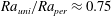 $\mathit{Ra}_{uni}/\mathit{Ra}_{per}\approx 0.75$
as it does not trigger secondary states. The reader may note that the system performance with secondary states may still be better than that achieved using purely spatially modulated heating. In figure 7(b) the strength of the uniform heating is expressed in absolute form, i.e. in terms of
$\mathit{Ra}_{uni}/\mathit{Ra}_{per}\approx 0.75$
as it does not trigger secondary states. The reader may note that the system performance with secondary states may still be better than that achieved using purely spatially modulated heating. In figure 7(b) the strength of the uniform heating is expressed in absolute form, i.e. in terms of
 $\mathit{Ra}_{uni}$
, as this might be better suited for experimental planning. A single state exists for
$\mathit{Ra}_{uni}$
, as this might be better suited for experimental planning. A single state exists for
 $\mathit{Ra}_{uni}<400$
for all values of
$\mathit{Ra}_{uni}<400$
for all values of
 $\mathit{Ra}_{per}$
. Within this range, the largest drag reduction is found for the largest values of
$\mathit{Ra}_{per}$
. Within this range, the largest drag reduction is found for the largest values of
 $\mathit{Ra}_{per}$
. A very rapid change occurs for
$\mathit{Ra}_{per}$
. A very rapid change occurs for
 $\mathit{Ra}_{per}\approx 400$
, where a small change of
$\mathit{Ra}_{per}\approx 400$
, where a small change of
 $\mathit{Ra}_{per}$
may result in a two- to threefold change of the pressure gradient correction. Stronger uniform heating (
$\mathit{Ra}_{per}$
may result in a two- to threefold change of the pressure gradient correction. Stronger uniform heating (
 $\mathit{Ra}_{uni}\geqslant 400$
) may lead to the formation of secondary states. The use of small
$\mathit{Ra}_{uni}\geqslant 400$
) may lead to the formation of secondary states. The use of small
 $\mathit{Ra}_{per}$
and large
$\mathit{Ra}_{per}$
and large
 $\mathit{Ra}_{uni}$
results in a large deterioration of the system performance (see the zone for
$\mathit{Ra}_{uni}$
results in a large deterioration of the system performance (see the zone for
 $\mathit{Ra}_{per}<300$
and
$\mathit{Ra}_{per}<300$
and
 $\mathit{Ra}_{uni}>400$
in figure 7
b). The use of much larger
$\mathit{Ra}_{uni}>400$
in figure 7
b). The use of much larger
 $\mathit{Ra}_{per}$
(
$\mathit{Ra}_{per}$
(
 $\mathit{Ra}_{per}>500$
) combined with large
$\mathit{Ra}_{per}>500$
) combined with large
 $\mathit{Ra}_{uni}$
eliminates secondary states and provides a very good system performance, e.g.
$\mathit{Ra}_{uni}$
eliminates secondary states and provides a very good system performance, e.g.
 $\mathit{Ra}_{per}$
combined with
$\mathit{Ra}_{per}$
combined with
 $\mathit{Ra}_{uni}=500$
almost triples the reduction of the pressure gradient achieved with
$\mathit{Ra}_{uni}=500$
almost triples the reduction of the pressure gradient achieved with
 $\mathit{Ra}_{uni}=0$
.
$\mathit{Ra}_{uni}=0$
.

Figure 7. Variations of the pressure gradient correction
 $A/\mathit{Re}$
as a function of
$A/\mathit{Re}$
as a function of
 $\mathit{Ra}_{per}$
for
$\mathit{Ra}_{per}$
for
 ${\it\alpha}=2$
and
${\it\alpha}=2$
and
 $\mathit{Re}=1$
for different levels of the uniform heating measured in terms of either
$\mathit{Re}=1$
for different levels of the uniform heating measured in terms of either
 $\mathit{Ra}_{uni}/\mathit{Ra}_{per}$
(a) or
$\mathit{Ra}_{uni}/\mathit{Ra}_{per}$
(a) or
 $\mathit{Ra}_{uni}$
(b).
$\mathit{Ra}_{uni}$
(b).
Figure 8 displays variations of
 $A/\mathit{Re}$
as a function of
$A/\mathit{Re}$
as a function of
 $\mathit{Ra}_{uni}$
for a fixed value of
$\mathit{Ra}_{uni}$
for a fixed value of
 $\mathit{Ra}_{per}$
. In figure 8(a) a relative measure of the intensity of uniform heating is used, i.e.
$\mathit{Ra}_{per}$
. In figure 8(a) a relative measure of the intensity of uniform heating is used, i.e.
 $\mathit{Ra}_{uni}/\mathit{Ra}_{per}$
. An initial improvement of the system performance due to an increase of
$\mathit{Ra}_{uni}/\mathit{Ra}_{per}$
. An initial improvement of the system performance due to an increase of
 $\mathit{Ra}_{uni}/\mathit{Ra}_{per}$
is followed by its deterioration if
$\mathit{Ra}_{uni}/\mathit{Ra}_{per}$
is followed by its deterioration if
 $\mathit{Ra}_{uni}/\mathit{Ra}_{per}$
becomes too large. Figure 9 illustrates changes in the flow topology due to an increase of
$\mathit{Ra}_{uni}/\mathit{Ra}_{per}$
becomes too large. Figure 9 illustrates changes in the flow topology due to an increase of
 $\mathit{Ra}_{uni}/\mathit{Ra}_{per}$
from 0 (point A in figure 8
a) to 0.5 (point B in figure 8
a) with
$\mathit{Ra}_{uni}/\mathit{Ra}_{per}$
from 0 (point A in figure 8
a) to 0.5 (point B in figure 8
a) with
 $\mathit{Ra}_{per}=800$
. An increase of the size of the separation bubbles is clearly visible and it correlates well with the increase of the intensity of motion from
$\mathit{Ra}_{per}=800$
. An increase of the size of the separation bubbles is clearly visible and it correlates well with the increase of the intensity of motion from
 ${\it\Psi}_{max}=3.6603$
to
${\it\Psi}_{max}=3.6603$
to
 ${\it\Psi}_{max}=6.8814$
. Drag reduction similar to that achieved with
${\it\Psi}_{max}=6.8814$
. Drag reduction similar to that achieved with
 $\mathit{Ra}_{per}=800$
and no uniform heating (
$\mathit{Ra}_{per}=800$
and no uniform heating (
 $\mathit{Ra}_{uni}=0$
) can also be achieved with
$\mathit{Ra}_{uni}=0$
) can also be achieved with
 $\mathit{Ra}_{uni}/\mathit{Ra}_{per}=2.44$
(point C in figure 8
a) and 3.92 (point E in figure 8
a), and a better reduction can be achieved with
$\mathit{Ra}_{uni}/\mathit{Ra}_{per}=2.44$
(point C in figure 8
a) and 3.92 (point E in figure 8
a), and a better reduction can be achieved with
 $\mathit{Ra}_{uni}/\mathit{Ra}_{per}=3.15$
(point D in figure 8
a). Secondary states exist for such conditions, and the corresponding flow topologies are displayed in figure 10. There are two layers of separation bubbles alternating with zones of the in-flow trapped fluid, resulting in the appearance of several stream tubes channelling fluid from left to right. There is no qualitative change in the flow topologies from
$\mathit{Ra}_{uni}/\mathit{Ra}_{per}=3.15$
(point D in figure 8
a). Secondary states exist for such conditions, and the corresponding flow topologies are displayed in figure 10. There are two layers of separation bubbles alternating with zones of the in-flow trapped fluid, resulting in the appearance of several stream tubes channelling fluid from left to right. There is no qualitative change in the flow topologies from
 $\mathit{Ra}_{uni}/\mathit{Ra}_{per}=2.44$
(figure 10
a) to
$\mathit{Ra}_{uni}/\mathit{Ra}_{per}=2.44$
(figure 10
a) to
 $\mathit{Ra}_{uni}/\mathit{Ra}_{per}=3.15$
(figure 10
b) where three separate stream tubes exist, while only two stream tubes remain at
$\mathit{Ra}_{uni}/\mathit{Ra}_{per}=3.15$
(figure 10
b) where three separate stream tubes exist, while only two stream tubes remain at
 $\mathit{Ra}_{uni}/\mathit{Ra}_{per}=3.92$
(figure 10
c). The delicate adjustment of the flow pattern results in the largest drag reduction for
$\mathit{Ra}_{uni}/\mathit{Ra}_{per}=3.92$
(figure 10
c). The delicate adjustment of the flow pattern results in the largest drag reduction for
 $\mathit{Ra}_{uni}/\mathit{Ra}_{per}=3.15$
(figure 10
b). It is remarkable that the same drag reduction can be achieved with the flow topology displayed in figure 9(a) as with the flow topologies shown in figure 10(a,c), while the topology displayed in figure 10(b) gives a better performance than the topology shown in figure 9(a).
$\mathit{Ra}_{uni}/\mathit{Ra}_{per}=3.15$
(figure 10
b). It is remarkable that the same drag reduction can be achieved with the flow topology displayed in figure 9(a) as with the flow topologies shown in figure 10(a,c), while the topology displayed in figure 10(b) gives a better performance than the topology shown in figure 9(a).

Figure 8. Variations of the pressure gradient correction
 $A/\mathit{Re}$
as a function of either
$A/\mathit{Re}$
as a function of either
 $\mathit{Ra}_{uni}/\mathit{Ra}_{per}$
(a) or
$\mathit{Ra}_{uni}/\mathit{Ra}_{per}$
(a) or
 $\mathit{Ra}_{uni}$
(b) for
$\mathit{Ra}_{uni}$
(b) for
 ${\it\alpha}=2$
and
${\it\alpha}=2$
and
 $\mathit{Re}=1$
for different values of
$\mathit{Re}=1$
for different values of
 $\mathit{Ra}_{per}$
. Flow topologies for conditions corresponding to points A and B in (a) are displayed in figure 9, topologies corresponding to points C, D, E in (a) are displayed in figure 10, topologies corresponding to points A, C, D in (b) are displayed in figure 11 and topologies for points E, F in (b) are displayed in figure 12.
$\mathit{Ra}_{per}$
. Flow topologies for conditions corresponding to points A and B in (a) are displayed in figure 9, topologies corresponding to points C, D, E in (a) are displayed in figure 10, topologies corresponding to points A, C, D in (b) are displayed in figure 11 and topologies for points E, F in (b) are displayed in figure 12.

Figure 9. Flow topologies for
 $\mathit{Re}=1$
,
$\mathit{Re}=1$
,
 ${\it\alpha}=2$
,
${\it\alpha}=2$
,
 $\mathit{Ra}_{per}=800$
and
$\mathit{Ra}_{per}=800$
and
 $\mathit{Ra}_{uni}/\mathit{Ra}_{per}=0$
(a,
$\mathit{Ra}_{uni}/\mathit{Ra}_{per}=0$
(a,
 ${\it\Psi}_{max}=3.6603$
) and 0.5 (b,
${\it\Psi}_{max}=3.6603$
) and 0.5 (b,
 ${\it\Psi}_{max}=6.8814$
). The corresponding flow conditions correspond to points A and B in figure 8(a).
${\it\Psi}_{max}=6.8814$
). The corresponding flow conditions correspond to points A and B in figure 8(a).

Figure 10. Flow topologies for
 $\mathit{Re}=1$
,
$\mathit{Re}=1$
,
 ${\it\alpha}=2$
,
${\it\alpha}=2$
,
 $\mathit{Ra}_{per}=800$
and
$\mathit{Ra}_{per}=800$
and
 $\mathit{Ra}_{uni}/\mathit{Ra}_{per}=2.44$
(a,
$\mathit{Ra}_{uni}/\mathit{Ra}_{per}=2.44$
(a,
 ${\it\Psi}_{max}=3.0877$
), 3.15 (b,
${\it\Psi}_{max}=3.0877$
), 3.15 (b,
 ${\it\Psi}_{max}=3.5442$
) and 3.92 (c,
${\it\Psi}_{max}=3.5442$
) and 3.92 (c,
 ${\it\Psi}_{max}=3.3575$
). The corresponding flow conditions correspond to points C, D, E in figure 8(a).
${\it\Psi}_{max}=3.3575$
). The corresponding flow conditions correspond to points C, D, E in figure 8(a).
Figure 8(b) displays variations of
 $A/\mathit{Re}$
as a function of
$A/\mathit{Re}$
as a function of
 $\mathit{Ra}_{uni}$
, and this offers an opportunity to discuss different strategies for an increase of
$\mathit{Ra}_{uni}$
, and this offers an opportunity to discuss different strategies for an increase of
 $A/\mathit{Re}$
in a potential experiment. Point A in this figure serves as a reference state where drag reduction of
$A/\mathit{Re}$
in a potential experiment. Point A in this figure serves as a reference state where drag reduction of
 $A/\mathit{Re}=0.13$
is achieved using purely spatially modulated heating with amplitude
$A/\mathit{Re}=0.13$
is achieved using purely spatially modulated heating with amplitude
 $\mathit{Ra}_{per}=500$
. The corresponding flow topology is displayed in figure 11(a) and the corresponding
$\mathit{Ra}_{per}=500$
. The corresponding flow topology is displayed in figure 11(a) and the corresponding
 ${\it\Psi}_{max}=2.6606$
. Further reduction of drag can be achieved by increasing
${\it\Psi}_{max}=2.6606$
. Further reduction of drag can be achieved by increasing
 $\mathit{Ra}_{per}$
while keeping
$\mathit{Ra}_{per}$
while keeping
 $\mathit{Ra}_{uni}$
unchanged, e.g. point B in figure 8(b) which corresponds to
$\mathit{Ra}_{uni}$
unchanged, e.g. point B in figure 8(b) which corresponds to
 $\mathit{Ra}_{per}=800$
and results in
$\mathit{Ra}_{per}=800$
and results in
 $A/\mathit{Re}=0.26$
and
$A/\mathit{Re}=0.26$
and
 ${\it\Psi}_{max}=3.6603$
; the corresponding flow topology is displayed in figure 9(a). An alternative method for decreasing the drag involves increasing
${\it\Psi}_{max}=3.6603$
; the corresponding flow topology is displayed in figure 9(a). An alternative method for decreasing the drag involves increasing
 $\mathit{Ra}_{uni}$
while keeping
$\mathit{Ra}_{uni}$
while keeping
 $\mathit{Ra}_{per}$
fixed. Points C and D in figure 8(b) correspond to
$\mathit{Ra}_{per}$
fixed. Points C and D in figure 8(b) correspond to
 $\mathit{Ra}_{per}=500$
and
$\mathit{Ra}_{per}=500$
and
 $\mathit{Ra}_{uni}=200$
, 400 respectively, and result in (
$\mathit{Ra}_{uni}=200$
, 400 respectively, and result in (
 $A/\mathit{Re}=0.35$
,
$A/\mathit{Re}=0.35$
,
 ${\it\Psi}_{max}=4.2444$
) and (
${\it\Psi}_{max}=4.2444$
) and (
 $A/\mathit{Re}=0.59$
,
$A/\mathit{Re}=0.59$
,
 ${\it\Psi}_{max}=6.0279$
); the resulting flow topologies are displayed in figure 11(b,c). A further increase of
${\it\Psi}_{max}=6.0279$
); the resulting flow topologies are displayed in figure 11(b,c). A further increase of
 $\mathit{Ra}_{uni}$
leads to the formation of secondary states but drag lower than the reference drag can still be achieved. Point E in figure 8(b) illustrates such a situation where
$\mathit{Ra}_{uni}$
leads to the formation of secondary states but drag lower than the reference drag can still be achieved. Point E in figure 8(b) illustrates such a situation where
 $\mathit{Ra}_{uni}=500$
was used, resulting in
$\mathit{Ra}_{uni}=500$
was used, resulting in
 $A/\mathit{Re}=0.25$
and
$A/\mathit{Re}=0.25$
and
 ${\it\Psi}_{max}=3.5033$
. The corresponding flow topology is displayed in figure 12(a). A further increase of
${\it\Psi}_{max}=3.5033$
. The corresponding flow topology is displayed in figure 12(a). A further increase of
 $\mathit{Ra}_{uni}$
complicates the flow structure and reduces the drag reduction. The drag reduction at
$\mathit{Ra}_{uni}$
complicates the flow structure and reduces the drag reduction. The drag reduction at
 $\mathit{Ra}_{uni}=590$
(point F in figure 8
b) is the same as for
$\mathit{Ra}_{uni}=590$
(point F in figure 8
b) is the same as for
 $\mathit{Ra}_{uni}=0$
(point A in figure 8
b), but the flow structure is very complex and involves two separate stream tubes, as shown in figure 12(b).
$\mathit{Ra}_{uni}=0$
(point A in figure 8
b), but the flow structure is very complex and involves two separate stream tubes, as shown in figure 12(b).

Figure 11. Flow topologies for
 $\mathit{Re}=1$
,
$\mathit{Re}=1$
,
 ${\it\alpha}=2$
,
${\it\alpha}=2$
,
 $\mathit{Ra}_{per}=500$
and
$\mathit{Ra}_{per}=500$
and
 $\mathit{Ra}_{uni}=0$
(a,
$\mathit{Ra}_{uni}=0$
(a,
 ${\it\Psi}_{max}=2.6606$
), 200 (b,
${\it\Psi}_{max}=2.6606$
), 200 (b,
 ${\it\Psi}_{max}=2.4244$
) and 400 (c,
${\it\Psi}_{max}=2.4244$
) and 400 (c,
 ${\it\Psi}_{max}=6.0279$
). The corresponding flow conditions correspond to points A, C, D in figure 8(b).
${\it\Psi}_{max}=6.0279$
). The corresponding flow conditions correspond to points A, C, D in figure 8(b).


Figure 13 provides aggregate information about the dependence of
 $A/\mathit{Re}$
on
$A/\mathit{Re}$
on
 ${\it\alpha}$
and
${\it\alpha}$
and
 $\mathit{Ra}_{per}$
. It can be seen that the highest drag reduction that can be achieved within the range of parameters studied is
$\mathit{Ra}_{per}$
. It can be seen that the highest drag reduction that can be achieved within the range of parameters studied is
 $A/\mathit{Re}\approx 0.3$
for
$A/\mathit{Re}\approx 0.3$
for
 $\mathit{Ra}_{uni}=0$
,
$\mathit{Ra}_{uni}=0$
,
 $A/\mathit{Re}\approx 1$
for
$A/\mathit{Re}\approx 1$
for
 $\mathit{Ra}_{uni}/\mathit{Ra}_{per}=0.5$
and
$\mathit{Ra}_{uni}/\mathit{Ra}_{per}=0.5$
and
 $A/\mathit{Re}>1$
for
$A/\mathit{Re}>1$
for
 $\mathit{Ra}_{uni}/\mathit{Ra}_{per}=1$
, although one must remember about the avoidance of secondary states in the latter case. The most effective heating wavenumber changes from
$\mathit{Ra}_{uni}/\mathit{Ra}_{per}=1$
, although one must remember about the avoidance of secondary states in the latter case. The most effective heating wavenumber changes from
 ${\it\alpha}\approx 1.8$
to
${\it\alpha}\approx 1.8$
to
 ${\it\alpha}\approx 2.1$
when
${\it\alpha}\approx 2.1$
when
 $\mathit{Ra}_{per}$
varies from 100 to 1000 and
$\mathit{Ra}_{per}$
varies from 100 to 1000 and
 $\mathit{Ra}_{uni}=0$
, it changes from
$\mathit{Ra}_{uni}=0$
, it changes from
 ${\it\alpha}\approx 1.8$
to
${\it\alpha}\approx 1.8$
to
 ${\it\alpha}\approx 2.5$
for
${\it\alpha}\approx 2.5$
for
 $\mathit{Ra}_{uni}/\mathit{Ra}_{per}=0.5$
and from
$\mathit{Ra}_{uni}/\mathit{Ra}_{per}=0.5$
and from
 ${\it\alpha}\approx 1.8$
to
${\it\alpha}\approx 1.8$
to
 ${\it\alpha}\approx 3$
for
${\it\alpha}\approx 3$
for
 $\mathit{Ra}_{uni}/\mathit{Ra}_{per}=1$
. Figure 14 provides aggregate information about the effects of Re. A rapid decrease of the drag reduction occurs for
$\mathit{Ra}_{uni}/\mathit{Ra}_{per}=1$
. Figure 14 provides aggregate information about the effects of Re. A rapid decrease of the drag reduction occurs for
 $\mathit{Re}>10$
regardless of the type of heating. As a matter of fact,
$\mathit{Re}>10$
regardless of the type of heating. As a matter of fact,
 $A/\mathit{Re}\approx 0.01$
for
$A/\mathit{Re}\approx 0.01$
for
 $\mathit{Re}=10$
for all cases considered. The most effective heating wavenumber is not affected by an increase of uniform heating.
$\mathit{Re}=10$
for all cases considered. The most effective heating wavenumber is not affected by an increase of uniform heating.

Figure 13. Variations of the pressure gradient correction
 $A/\mathit{Re}$
as a function of
$A/\mathit{Re}$
as a function of
 ${\it\alpha}$
and
${\it\alpha}$
and
 $\mathit{Ra}_{per}$
for the uniform heating corresponding to
$\mathit{Ra}_{per}$
for the uniform heating corresponding to
 $\mathit{Ra}_{uni}/\mathit{Ra}_{per}=0$
, 0.5, 1 (a–c respectively) for
$\mathit{Ra}_{uni}/\mathit{Ra}_{per}=0$
, 0.5, 1 (a–c respectively) for
 $\mathit{Re}=1$
.
$\mathit{Re}=1$
.

Figure 14. Variations of the pressure gradient correction
 $A/\mathit{Re}$
as a function of
$A/\mathit{Re}$
as a function of
 ${\it\alpha}$
and
${\it\alpha}$
and
 $\mathit{Re}$
for
$\mathit{Re}$
for
 $\mathit{Ra}_{per}=500$
and
$\mathit{Ra}_{per}=500$
and
 $\mathit{Ra}_{uni}=0$
, 0.5, 0.75 (a–c respectively).
$\mathit{Ra}_{uni}=0$
, 0.5, 0.75 (a–c respectively).
Figure 15 displays variations of
 $A/\mathit{Re}$
as a function of
$A/\mathit{Re}$
as a function of
 $\mathit{Ra}_{per}$
and
$\mathit{Ra}_{per}$
and
 $\mathit{Ra}_{uni}$
and provides information about the best combination of both types of heating. It can be seen that the best system performance corresponds to the largest
$\mathit{Ra}_{uni}$
and provides information about the best combination of both types of heating. It can be seen that the best system performance corresponds to the largest
 $\mathit{Ra}_{per}$
and the largest
$\mathit{Ra}_{per}$
and the largest
 $\mathit{Ra}_{uni}$
. Secondary states are generated when
$\mathit{Ra}_{uni}$
. Secondary states are generated when
 $\mathit{Ra}_{uni}$
is large but
$\mathit{Ra}_{uni}$
is large but
 $\mathit{Ra}_{per}$
is not sufficiently large (right bottom corner in figure 15); such conditions should be avoided as they result in deterioration of the system performance. The same figure provides information about the heating conditions at the lower wall. Local cooling is avoided when
$\mathit{Ra}_{per}$
is not sufficiently large (right bottom corner in figure 15); such conditions should be avoided as they result in deterioration of the system performance. The same figure provides information about the heating conditions at the lower wall. Local cooling is avoided when
 $\mathit{Ra}_{uni}/\mathit{Ra}_{per}>0.5$
and this is very important in applications. Secondary flows can be avoided for
$\mathit{Ra}_{uni}/\mathit{Ra}_{per}>0.5$
and this is very important in applications. Secondary flows can be avoided for
 $\mathit{Ra}_{uni}/\mathit{Ra}_{per}<1$
. The zone between these two limits is likely to be of the most importance in applications.
$\mathit{Ra}_{uni}/\mathit{Ra}_{per}<1$
. The zone between these two limits is likely to be of the most importance in applications.

Figure 15. Variations of the pressure gradient correction
 $A/\mathit{Re}$
as a function of
$A/\mathit{Re}$
as a function of
 $\mathit{Ra}_{per}$
and
$\mathit{Ra}_{per}$
and
 $\mathit{Ra}_{uni}$
for
$\mathit{Ra}_{uni}$
for
 ${\it\alpha}=2$
and
${\it\alpha}=2$
and
 $\mathit{Re}=1$
. Solid lines represent isolines of
$\mathit{Re}=1$
. Solid lines represent isolines of
 $A/\mathit{Re}$
and dashed lines identify locations of
$A/\mathit{Re}$
and dashed lines identify locations of
 $\mathit{Ra}_{per}/\mathit{Re}_{uni}=\text{const.}$
in the (
$\mathit{Ra}_{per}/\mathit{Re}_{uni}=\text{const.}$
in the (
 $\mathit{Ra}_{per}$
,
$\mathit{Ra}_{per}$
,
 $\mathit{Ra}_{uni}$
) plane.
$\mathit{Ra}_{uni}$
) plane.
6.3. Analysis of heat transfer
The net heat transfer across the channel resulting from the applied heating is illustrated in figure 16, which displays variations of the average Nusselt number
 $\mathit{Nu}_{av}$
based on the temperature scale
$\mathit{Nu}_{av}$
based on the temperature scale
 $T_{per}$
and defined as
$T_{per}$
and defined as
 $$\begin{eqnarray}\mathit{Nu}_{av}=\frac{1}{{\it\lambda}}\int _{0}^{{\it\lambda}}\left(\left.\frac{\text{d}{\it\theta}_{T}}{\text{d}y}\right|_{y=-1}\right)\text{d}x=\frac{\mathit{Ra}_{uni}}{2\mathit{Ra}_{per}}-\left.\frac{\text{d}{\it\phi}^{(0)}}{\text{d}y}\right|_{y=-1},\end{eqnarray}$$
as a function of
 ${\it\alpha}$
and
${\it\alpha}$
and
 $\mathit{Ra}_{per}$
for
$\mathit{Ra}_{per}$
for
 $\mathit{Ra}_{uni}/\mathit{Ra}_{per}=0$
, 0.5, 1 and for
$\mathit{Ra}_{uni}/\mathit{Ra}_{per}=0$
, 0.5, 1 and for
 $\mathit{Re}=1$
, i.e. for the same conditions as used in figure 14 for illustration of variations of the pressure gradient reduction. This heat flow is driven mostly by conduction (compare figure 16
a with figure 16
b,c) and might be viewed as an energy loss. The largest heat flow occurs for
$\mathit{Re}=1$
, i.e. for the same conditions as used in figure 14 for illustration of variations of the pressure gradient reduction. This heat flow is driven mostly by conduction (compare figure 16
a with figure 16
b,c) and might be viewed as an energy loss. The largest heat flow occurs for
 ${\it\alpha}\approx 1{-}1.5$
while the largest pressure gradient reduction is found for
${\it\alpha}\approx 1{-}1.5$
while the largest pressure gradient reduction is found for
 ${\it\alpha}\approx 2{-}2.5$
, and this suggests that a judicious selection of
${\it\alpha}\approx 2{-}2.5$
, and this suggests that a judicious selection of
 ${\it\alpha}$
can be used to reduce the energy cost. The real role of transverse heat flow is, however, more complex. To illustrate this point, consider a channel with the upper wall insulated, which eliminates this heat flow. The formulation of the corresponding problem is given in appendix D and the resulting field equations have been solved using the same technique as described in § 3. The results presented in figure 17 demonstrate up to 50 % reduction of the pressure gradient correction when the isothermal upper wall is replaced with an insulated wall (compare figure 16
a with figure 17). This suggests that a higher drag reduction is achieved when heating creates both large horizontal and large vertical temperature gradients; if one is interested in a high drag reduction, the energy costs associated with the creation of such gradients must be accepted. This point is well illustrated by comparing figure 17 with figure 14(a–c) in this particular order as it corresponds to progressively larger vertical temperature gradients combined with the same horizontal gradients.
${\it\alpha}$
can be used to reduce the energy cost. The real role of transverse heat flow is, however, more complex. To illustrate this point, consider a channel with the upper wall insulated, which eliminates this heat flow. The formulation of the corresponding problem is given in appendix D and the resulting field equations have been solved using the same technique as described in § 3. The results presented in figure 17 demonstrate up to 50 % reduction of the pressure gradient correction when the isothermal upper wall is replaced with an insulated wall (compare figure 16
a with figure 17). This suggests that a higher drag reduction is achieved when heating creates both large horizontal and large vertical temperature gradients; if one is interested in a high drag reduction, the energy costs associated with the creation of such gradients must be accepted. This point is well illustrated by comparing figure 17 with figure 14(a–c) in this particular order as it corresponds to progressively larger vertical temperature gradients combined with the same horizontal gradients.

Figure 16. Variations of the average Nusselt number
 $\mathit{Nu}_{av}$
as a function of
$\mathit{Nu}_{av}$
as a function of
 ${\it\alpha}$
and
${\it\alpha}$
and
 $\mathit{Ra}_{per}$
for
$\mathit{Ra}_{per}$
for
 $\mathit{Ra}_{uni}/\mathit{Ra}_{per}=0$
, 0.5, 1 (a–c respectively) for
$\mathit{Ra}_{uni}/\mathit{Ra}_{per}=0$
, 0.5, 1 (a–c respectively) for
 $\mathit{Re}=1$
.
$\mathit{Re}=1$
.

Figure 17. Variations of the pressure gradient correction
 $A/\mathit{Re}$
for
$A/\mathit{Re}$
for
 $\mathit{Re}=1$
as a function of
$\mathit{Re}=1$
as a function of
 ${\it\alpha}$
and
${\it\alpha}$
and
 $\mathit{Ra}_{per}$
for a channel with an insulated upper wall and subject to periodic heating at the lower wall.
$\mathit{Ra}_{per}$
for a channel with an insulated upper wall and subject to periodic heating at the lower wall.
Information about the horizontal heat flow is gained by looking at the heat flux leaving the lower wall per half heating wavelength. It is convenient to express this heat flux in terms of the Nusselt number
 $\mathit{Nu}_{h}$
, defined as
$\mathit{Nu}_{h}$
, defined as
 $$\begin{eqnarray}\displaystyle \mathit{Nu}_{h} & = & \displaystyle \frac{2}{{\it\lambda}}\mathit{Pr}\int _{-{\it\lambda}/4}^{{\it\lambda}/4}\left.\left(\frac{\partial {\it\theta}_{T}}{\partial y}\right)\right|_{y=-1}=\left\{\frac{\mathit{Ra}_{uni}}{2\mathit{Ra}_{per}}\right\}+\Bigg\{\frac{{\it\alpha}}{2{\rm\pi}}[\coth ({\it\alpha})+\tanh ({\it\alpha})]\Bigg\}\nonumber\\ \displaystyle & & \displaystyle -\,\left\{\frac{2}{{\it\lambda}}\mathit{Pr}\int _{-{\it\lambda}/4}^{{\it\lambda}/4}\left(\left.\frac{\partial {\it\theta}_{1}}{\partial y}\right|_{y=-1}\right)\text{d}x\right\},\end{eqnarray}$$
where the first term on the right-hand side accounts for the conduction due to the uniform heating, the second one accounts for the conduction due to the periodic heating and the third one accounts for the convective effects. Figure 18 displays variations of
 $\mathit{Nu}_{h}$
as a function of
$\mathit{Nu}_{h}$
as a function of
 $\mathit{Ra}_{per}$
and
$\mathit{Ra}_{per}$
and
 ${\it\alpha}$
, while figure 19 displays variations of the convective effects only, i.e. the third term in (6.18). It can be seen that the horizontal heat fluxes are much larger than the net heat flow across the channel (compare figure 18 with figure 16), with conductive effects providing the largest contribution (compare figure 18 with figure 19). It may be concluded that the main energy cost is associated with the creation of the horizontal temperature gradients.
${\it\alpha}$
, while figure 19 displays variations of the convective effects only, i.e. the third term in (6.18). It can be seen that the horizontal heat fluxes are much larger than the net heat flow across the channel (compare figure 18 with figure 16), with conductive effects providing the largest contribution (compare figure 18 with figure 19). It may be concluded that the main energy cost is associated with the creation of the horizontal temperature gradients.

Figure 18. Variations of the Nusselt number for the half heating wavelength
 $\mathit{Nu}_{h}$
(see (6.18)) as a function of
$\mathit{Nu}_{h}$
(see (6.18)) as a function of
 ${\it\alpha}$
and
${\it\alpha}$
and
 $\mathit{Ra}_{per}$
for
$\mathit{Ra}_{per}$
for
 $\mathit{Ra}_{uni}/\mathit{Ra}_{per}=0$
, 0.5 (a,b respectively) for
$\mathit{Ra}_{uni}/\mathit{Ra}_{per}=0$
, 0.5 (a,b respectively) for
 $\mathit{Re}=1$
.
$\mathit{Re}=1$
.

Figure 19. Variations of the convective component of the Nusselt number for the half heating wavelength
 $\mathit{Nu}_{h}$
(see the third term on the right-hand side of (6.18)) as a function of
$\mathit{Nu}_{h}$
(see the third term on the right-hand side of (6.18)) as a function of
 ${\it\alpha}$
and
${\it\alpha}$
and
 $\mathit{Ra}_{per}$
for
$\mathit{Ra}_{per}$
for
 $\mathit{Ra}_{uni}/\mathit{Ra}_{per}=0$
, 0.5 (a,b respectively) for
$\mathit{Ra}_{uni}/\mathit{Ra}_{per}=0$
, 0.5 (a,b respectively) for
 $\mathit{Re}=1$
.
$\mathit{Re}=1$
.
The results presented in this paper suggest the use of spatially modulated heating as a method for intensification and/or optimization of the heat transfer, which is typically measured in terms of the ratio of the transverse heat flux and the pressure gradient required to maintain the flow (Fiebig Reference Fiebig1995; Jacobi & Shah Reference Jacobi and Shah1998; Ligrani, Oliviera & Blaskovich Reference Ligrani, Oliviera and Blaskovich2003). The heat flow in the case of uniform heating is driven under subcritical conditions by conduction only; one can increase its magnitude by using the supercritical conditions but at a cost of increased pressure loss (Gage & Reid Reference Gage and Reid1968). The heat flow in the case of spatially modulated heating increases above its conductive base level and, at the same time, the pressure gradient decreases below the isothermal reference level. The gains are similar to those reported by Yamamoto, Hasegawa & Kasagi (Reference Yamamoto, Hasegawa and Kasagi2013), who achieved simultaneous drag reduction and heat transfer enhancement in turbulent flow using wall waves of suction/blowing travelling in the downstream direction. The present system is simpler due to its passive character.
The question of net gain, i.e. determination whether the reduction of the drag overcomes the costs of the heating, is difficult to answer. It has been shown that the overall viscous dissipation in an isothermal channel under a constant flow rate reaches a minimum for a laminar parabolic profile (Bewley Reference Bewley2009; Fukugata, Sugiyama & Kasagi Reference Fukugata, Sugiyama and Kasagi2009), and thus the overall energy consumption is always higher for controlled flow than for uncontrolled flow. This statement remains to be proven for a non-isothermal flow but probably remains valid. The cost of heating is a strong function of the heating technique but could be marginal if the heat supply were sufficiently inexpensive, e.g. waste heat. One can also look at the heating-induced drag reduction as an alternative pumping method where the total required pressure difference between the entrance and exit from the conduit is partially replaced by the heating-induced propulsive force distributed along the channel length. This pumping method may prove to be advantageous for long conduits and may provide an alternative to peristaltic pumping (Takagi & Balmforth Reference Takagi and Balmforth2011).
Our analysis has been carried out using the Boussinesq approximation and one needs to look at the limits of its applicability. The critical value of
 $\mathit{Ra}_{uni}$
required to induce natural convection in the case of a uniformly heated lower wall and using the Boussinesq fluid model is
$\mathit{Ra}_{uni}$
required to induce natural convection in the case of a uniformly heated lower wall and using the Boussinesq fluid model is
 $\mathit{Ra}_{uni,cr}=213.5$
; this value has been confirmed in numerous experiments (Gage & Reid Reference Gage and Reid1968). The analysis described in this paper considered
$\mathit{Ra}_{uni,cr}=213.5$
; this value has been confirmed in numerous experiments (Gage & Reid Reference Gage and Reid1968). The analysis described in this paper considered
 $\mathit{Ra}_{uni}<1000$
and
$\mathit{Ra}_{uni}<1000$
and
 $\mathit{Ra}_{per}<1000$
, with the bulk of the results obtained for
$\mathit{Ra}_{per}<1000$
, with the bulk of the results obtained for
 $\mathit{Ra}_{uni}<400$
,
$\mathit{Ra}_{uni}<400$
,
 $\mathit{Ra}_{per}<500$
, where the Boussinesq approximation should be able to capture the basic mechanisms. The more extreme parameter values probably enter into the zone where real gas effects become important but are included in this presentation in order to illustrate the physical trends. It remains to be determined what role real gas effects play and under what conditions they need to be accounted for.
$\mathit{Ra}_{per}<500$
, where the Boussinesq approximation should be able to capture the basic mechanisms. The more extreme parameter values probably enter into the zone where real gas effects become important but are included in this presentation in order to illustrate the physical trends. It remains to be determined what role real gas effects play and under what conditions they need to be accounted for.
It is useful to return to dimensional quantities in order to assist with the interpretation of the results. The presented results have been obtained with
 $\mathit{Pr}=0.71$
(air). We now assume atmospheric pressure and a reference temperature of
$\mathit{Pr}=0.71$
(air). We now assume atmospheric pressure and a reference temperature of
 $T_{ref}=17~^{\circ }\text{C}$
to obtain a conductivity
$T_{ref}=17~^{\circ }\text{C}$
to obtain a conductivity
 $k=0.0263~(\text{W}~\text{m}^{-1}~\text{K}^{-1})$
, specific heat
$k=0.0263~(\text{W}~\text{m}^{-1}~\text{K}^{-1})$
, specific heat
 $c=1007~(\text{J}~\text{kg}^{-1}~\text{K}^{-1})$
, thermal diffusivity
$c=1007~(\text{J}~\text{kg}^{-1}~\text{K}^{-1})$
, thermal diffusivity
 ${\it\kappa}=k/{\it\rho}c=22.5\times 10^{-6}~(\text{m}^{2}~\text{s}^{-1})$
, dynamic viscosity
${\it\kappa}=k/{\it\rho}c=22.5\times 10^{-6}~(\text{m}^{2}~\text{s}^{-1})$
, dynamic viscosity
 ${\it\mu}=184.6\times 10^{-7}~(\text{N}~\text{s}~\text{m}^{-2})$
, kinematic viscosity
${\it\mu}=184.6\times 10^{-7}~(\text{N}~\text{s}~\text{m}^{-2})$
, kinematic viscosity
 ${\it\nu}=15.89\times 10^{-6}~(\text{m}^{2}~\text{s}^{-1})$
, density
${\it\nu}=15.89\times 10^{-6}~(\text{m}^{2}~\text{s}^{-1})$
, density
 ${\it\rho}=1.1614~(\text{kg}~\text{m}^{-3})$
, thermal expansion coefficient
${\it\rho}=1.1614~(\text{kg}~\text{m}^{-3})$
, thermal expansion coefficient
 ${\it\Gamma}=1/(17+273)=1/300~(\text{K}^{-1})$
and gravitational acceleration
${\it\Gamma}=1/(17+273)=1/300~(\text{K}^{-1})$
and gravitational acceleration
 $g=9.81~(\text{m}~\text{s}^{-2})$
(Bergman et al.
Reference Bergman, Lavine, Incropera and Dewitt2011). This leads to
$g=9.81~(\text{m}~\text{s}^{-2})$
(Bergman et al.
Reference Bergman, Lavine, Incropera and Dewitt2011). This leads to
 $\mathit{Ra}_{uni}=g{\it\Gamma}h^{3}T_{uni}/{\it\nu}{\it\kappa}=91.146\times 10^{6}h^{3}T_{uni}$
and
$\mathit{Ra}_{uni}=g{\it\Gamma}h^{3}T_{uni}/{\it\nu}{\it\kappa}=91.146\times 10^{6}h^{3}T_{uni}$
and
 $\mathit{Ra}_{per}=g{\it\Gamma}h^{3}T_{per}/{\it\nu}{\it\kappa}=91.146\times 10^{6}h^{3}T_{per}$
. If we assume a permissible temperature difference of
$\mathit{Ra}_{per}=g{\it\Gamma}h^{3}T_{per}/{\it\nu}{\it\kappa}=91.146\times 10^{6}h^{3}T_{per}$
. If we assume a permissible temperature difference of
 ${\rm\Delta}T=10~^{\circ }\text{C}$
(
${\rm\Delta}T=10~^{\circ }\text{C}$
(
 $T_{uni}=T_{per}=10~^{\circ }\text{C}$
) we obtain
$T_{uni}=T_{per}=10~^{\circ }\text{C}$
) we obtain
 $\mathit{Ra}_{uni}=\mathit{Ra}_{per}=914.6\times 10^{6}h^{3}$
. Assuming
$\mathit{Ra}_{uni}=\mathit{Ra}_{per}=914.6\times 10^{6}h^{3}$
. Assuming
 $\mathit{Ra}_{uni}=\mathit{Ra}_{per}=200$
leads to
$\mathit{Ra}_{uni}=\mathit{Ra}_{per}=200$
leads to
 $h=0.006~(\text{m})$
. The same calculation for
$h=0.006~(\text{m})$
. The same calculation for
 $\mathit{Ra}_{uni}=\mathit{Ra}_{per}=500$
leads to
$\mathit{Ra}_{uni}=\mathit{Ra}_{per}=500$
leads to
 $h=0.0095~(\text{m})$
. Doubling the permissible temperature difference to
$h=0.0095~(\text{m})$
. Doubling the permissible temperature difference to
 ${\rm\Delta}T=20~^{\circ }\text{C}$
leads to
${\rm\Delta}T=20~^{\circ }\text{C}$
leads to
 $h=0.004\,79~(\text{m})$
for
$h=0.004\,79~(\text{m})$
for
 $\mathit{Ra}_{uni}=\mathit{Ra}_{per}=200$
and
$\mathit{Ra}_{uni}=\mathit{Ra}_{per}=200$
and
 $h=0.0065~(\text{m})$
for
$h=0.0065~(\text{m})$
for
 $\mathit{Ra}_{uni}=\mathit{Ra}_{per}=500$
. The present results are, thus, applicable to channels with heights of a few millimetres. A proper account of real gas effects should provide means for expansion of the applicability of the results to a wider range of temperature differences.
$\mathit{Ra}_{uni}=\mathit{Ra}_{per}=500$
. The present results are, thus, applicable to channels with heights of a few millimetres. A proper account of real gas effects should provide means for expansion of the applicability of the results to a wider range of temperature differences.
7. Summary
The reduction of pressure losses in a pressure-driven flow in a heated channel has been analysed. Detailed quantitative results have been presented for the Prandtl number
 $\mathit{Pr}=0.71$
, which well approximates the properties of air. The heating has to have a spatially modulated component in order to reduce pressure losses. This heating generates a buoyancy field; this leads to the formation of separation bubbles which isolate the stream from direct contact with the bounding wall. The buoyancy force drives motion inside the bubbles; this generates a propulsive force which contributes to reduction of the pressure loss. The drag reducing effect can be magnified by increasing the vertical and horizontal temperature gradients as this would lead to a more intense convection. It has been demonstrated that use of a proper combination of spatially modulated heating and spatially uniform heating produces the desired effect and the drag reduction can be increased almost threefold (compared with the drag reduction achieved without uniform heating) within the range of parameters studied. The use of an excessively large uniform heating component leads to the formation of secondary states, and this causes a significant drop in the reduction of pressure losses. The use of large modulated heating together with large uniform heating avoids the creation of secondary states and provides the best opportunity for the reduction of pressure losses. Use of large uniform heating and small modulated heating should be avoided. The appearance of secondary states does not necessarily imply a deterioration of the system performance below that achieved using purely modulated heating; such a system may have pressure losses smaller than those achieved with purely modulated heating, and this offers opportunities for many applications. It has been shown that the drag reducing effect is negligible for heating with long-wavelength spatial modulations as well as with short-wavelength modulations. It has also been shown that the drag reducing effect rapidly decreases when the flow Reynolds number exceeds
$\mathit{Pr}=0.71$
, which well approximates the properties of air. The heating has to have a spatially modulated component in order to reduce pressure losses. This heating generates a buoyancy field; this leads to the formation of separation bubbles which isolate the stream from direct contact with the bounding wall. The buoyancy force drives motion inside the bubbles; this generates a propulsive force which contributes to reduction of the pressure loss. The drag reducing effect can be magnified by increasing the vertical and horizontal temperature gradients as this would lead to a more intense convection. It has been demonstrated that use of a proper combination of spatially modulated heating and spatially uniform heating produces the desired effect and the drag reduction can be increased almost threefold (compared with the drag reduction achieved without uniform heating) within the range of parameters studied. The use of an excessively large uniform heating component leads to the formation of secondary states, and this causes a significant drop in the reduction of pressure losses. The use of large modulated heating together with large uniform heating avoids the creation of secondary states and provides the best opportunity for the reduction of pressure losses. Use of large uniform heating and small modulated heating should be avoided. The appearance of secondary states does not necessarily imply a deterioration of the system performance below that achieved using purely modulated heating; such a system may have pressure losses smaller than those achieved with purely modulated heating, and this offers opportunities for many applications. It has been shown that the drag reducing effect is negligible for heating with long-wavelength spatial modulations as well as with short-wavelength modulations. It has also been shown that the drag reducing effect rapidly decreases when the flow Reynolds number exceeds
 $\mathit{Re}=10$
, regardless of whether the uniform heating is used or not. The magnitude of drag reduction can reach up to 75 % of the isothermal value.
$\mathit{Re}=10$
, regardless of whether the uniform heating is used or not. The magnitude of drag reduction can reach up to 75 % of the isothermal value.
The reader may note that identification of the net energy effect and determination of whether or not it is favourable require a system-level study, which must include the costs of producing the desired wall temperature distribution as well as the required energy input.
There is a need for experimental verification of our predictions. The heating strategy analysed in this paper provides a basis for the design of an effective experiment as the results show that local cooling is not required; the desired effect can be achieved simply by using non-uniform heating along the lower wall.
Acknowledgements
This work has been carried out with support from the Natural Sciences and Engineering Research Council (NSERC) of Canada. The authors would like to thank Dr E. Savory for proofreading of the manuscript.
Appendix A
Definitions of functions used in § 4:
 $$\begin{eqnarray}\displaystyle \hat{\hat{{\it\theta}}}_{00} & = & \displaystyle \frac{1}{4}-\frac{y}{4},\end{eqnarray}$$
 $$\begin{eqnarray}\displaystyle \hat{\hat{{\it\theta}}}_{02} & = & \displaystyle -\frac{y^{3}}{24}+\frac{y^{2}}{8}+\frac{y}{24}-\frac{1}{8},\end{eqnarray}$$
 $$\begin{eqnarray}\displaystyle \hat{\hat{{\it\theta}}}_{04} & = & \displaystyle -\frac{y^{5}}{480}+\frac{y^{4}}{96}+\frac{y^{3}}{144}-\frac{y^{2}}{16}-\frac{7y}{1440}+\frac{5}{96},\end{eqnarray}$$
 $$\begin{eqnarray}\displaystyle F_{U1}(y) & = & \displaystyle \frac{y^{4}}{96}-\frac{y^{3}}{24}-\frac{y^{2}}{80}+\frac{y}{24}+\frac{1}{480},\end{eqnarray}$$
 $$\begin{eqnarray}\displaystyle F_{V2}(y) & = & \displaystyle -\frac{y^{5}}{480}+\frac{y^{4}}{96}+\frac{y^{3}}{240}-\frac{y^{2}}{48}-\frac{y}{480}+\frac{1}{96},\end{eqnarray}$$
 $$\begin{eqnarray}\displaystyle F_{P0}(y) & = & \displaystyle -\frac{y^{2}}{8}+\frac{y}{4}+\frac{1}{40},\end{eqnarray}$$
 $$\begin{eqnarray}\displaystyle F_{{\it\Theta}1} & = & \displaystyle -\frac{y^{5}}{80}+\frac{y^{4}}{48}+\frac{y^{3}}{24}-\frac{y^{2}}{8}-\frac{7y}{240}+\frac{5}{48},\end{eqnarray}$$
 $$\begin{eqnarray}\displaystyle F_{U21}(y) & = & \displaystyle -\frac{y^{8}}{26\,880}+\frac{y^{7}}{10\,080}+\frac{y^{6}}{2880}-\frac{y^{5}}{480}-\frac{7y^{4}}{5760}\nonumber\\ \displaystyle & & \displaystyle +\,\frac{5y^{3}}{288}+\frac{107y^{2}}{100\,800}-\frac{31y}{2016}-\frac{1}{6400},\end{eqnarray}$$
 $$\begin{eqnarray}\displaystyle F_{U22}(y) & = & \displaystyle -\frac{y^{8}}{8960}+\frac{y^{7}}{2016}+\frac{7y^{6}}{14\,400}-\frac{y^{5}}{480}-\frac{y^{4}}{1152}+\frac{y^{3}}{288}\nonumber\\ \displaystyle & & \displaystyle +\,\frac{19y^{2}}{33\,600}-\frac{19y}{10\,080}-\frac{29}{403\,200},\end{eqnarray}$$
 $$\begin{eqnarray}\displaystyle F_{V31}(y) & = & \displaystyle -\frac{y^{9}}{241\,920}+\frac{y^{8}}{80\,640}+\frac{y^{7}}{20\,160}-\frac{y^{6}}{2880}-\frac{7y^{5}}{28\,800}+\frac{5y^{4}}{1152}\nonumber\\ \displaystyle & & \displaystyle +\,\frac{107y^{3}}{302\,400}-\frac{31y^{2}}{4032}-\frac{y}{6400}+\frac{33}{8960},\end{eqnarray}$$
 $$\begin{eqnarray}\displaystyle F_{V32}(y) & = & \displaystyle -\frac{y^{9}}{80\,640}+\frac{y^{8}}{16\,128}+\frac{y^{7}}{14\,400}-\frac{y^{6}}{2880}-\frac{y^{5}}{5760}+\frac{y^{4}}{1152}\nonumber\\ \displaystyle & & \displaystyle +\,\frac{19y^{3}}{100\,800}-\frac{19y^{2}}{20\,160}-\frac{29y}{403\,200}+\frac{29}{80\,640},\end{eqnarray}$$
 $$\begin{eqnarray}\displaystyle F_{P1} & = & \displaystyle -\frac{y^{6}}{480}+\frac{y^{5}}{240}+\frac{y^{4}}{96}-\frac{y^{3}}{24}-\frac{7y^{2}}{480}+\frac{5y}{48}+\frac{107}{50\,400},\end{eqnarray}$$
 $$\begin{eqnarray}\displaystyle F_{{\it\Theta}21} & = & \displaystyle \frac{y^{7}}{26\,880}-\frac{y^{6}}{3840}+\frac{y^{5}}{6400}+\frac{y^{4}}{1280}-\frac{y^{3}}{1280}\nonumber\\ \displaystyle & & \displaystyle -\,\frac{y^{2}}{1280}+\frac{79}{134\,400}y+\frac{1}{3840},\end{eqnarray}$$
 $$\begin{eqnarray}\displaystyle F_{{\it\Theta}22} & = & \displaystyle \frac{1}{201\,600}\big(5y^{7}-35y^{6}-21y^{5}+175y^{4}+35y^{3}-525y^{2}-19y+385\big),\qquad\end{eqnarray}$$
 $$\begin{eqnarray}\displaystyle F_{{\it\Theta}23} & = & \displaystyle \frac{1}{201\,600}\big(35y^{9}-75y^{8}-260y^{7}+980y^{6}+714y^{5}-3850y^{4}\nonumber\\ \displaystyle & & \displaystyle -\,980y^{3}+10\,500y^{2}+491y-7555\big),\end{eqnarray}$$
 $$\begin{eqnarray}\displaystyle F_{{\it\Theta}24} & = & \displaystyle -\frac{y^{7}}{40\,320}+\frac{y^{6}}{5760}-\frac{y^{5}}{4800}-\frac{y^{4}}{2880}+\frac{y^{3}}{1152}\nonumber\\ \displaystyle & & \displaystyle -\,\frac{y^{2}}{1920}-\frac{1}{1575}y+\frac{1}{1440}.\end{eqnarray}$$
Appendix B
Definitions of functions used in § 5:
 $$\begin{eqnarray}\displaystyle & G_{U41}({\it\eta})={\textstyle \frac{1}{192}}(24{\it\eta}+6{\it\eta}^{2}+2{\it\eta}^{3}-{\it\eta}^{4}), & \displaystyle\end{eqnarray}$$
 $$\begin{eqnarray}\displaystyle & G_{U42}({\it\eta})={\textstyle \frac{1}{192}}(30{\it\eta}+3{\it\eta}^{2}-2{\it\eta}^{3}-{\it\eta}^{4}), & \displaystyle\end{eqnarray}$$
 $$\begin{eqnarray}\displaystyle & G_{V41}({\it\eta})={\textstyle \frac{1}{192}}(12{\it\eta}^{2}+6{\it\eta}^{3}+2{\it\eta}^{4}), & \displaystyle\end{eqnarray}$$
 $$\begin{eqnarray}\displaystyle & G_{V42}({\it\eta})={\textstyle \frac{1}{192}}(15{\it\eta}^{2}+6{\it\eta}^{3}+{\it\eta}^{4}), & \displaystyle\end{eqnarray}$$
 $$\begin{eqnarray}\displaystyle & G_{P31}({\it\eta})={\textstyle \frac{1}{96}}(18+6{\it\eta}+6{\it\eta}^{2}+4{\it\eta}^{3}), & \displaystyle\end{eqnarray}$$
 $$\begin{eqnarray}\displaystyle & G_{P32}({\it\eta})={\textstyle \frac{1}{96}}(27+12{\it\eta}-4{\it\eta}^{2}), & \displaystyle\end{eqnarray}$$
 $$\begin{eqnarray}\displaystyle & G_{{\it\Theta}41}({\it\eta})={\textstyle \frac{1}{384}}(3{\it\eta}+3{\it\eta}^{2}+2{\it\eta}^{3}), & \displaystyle\end{eqnarray}$$
 $$\begin{eqnarray}\displaystyle & G_{{\it\Theta}42}({\it\eta})={\textstyle \frac{1}{48}}(15+15{\it\eta}+10{\it\eta}^{2}+3{\it\eta}^{3}), & \displaystyle\end{eqnarray}$$
 $$\begin{eqnarray}\displaystyle & G_{U51}({\it\eta})=-360{\it\eta}-90{\it\eta}^{2}-30{\it\eta}^{3}+6{\it\eta}^{5}, & \displaystyle\end{eqnarray}$$
 $$\begin{eqnarray}\displaystyle & G_{U52}({\it\eta})=-270{\it\eta}-45{\it\eta}^{2}+5{\it\eta}^{4}+2{\it\eta}^{5}, & \displaystyle\end{eqnarray}$$
 $$\begin{eqnarray}\displaystyle & G_{U53}({\it\eta})=3{\it\eta}-3{\it\eta}^{2}-8{\it\eta}^{3}+4{\it\eta}^{4}, & \displaystyle\end{eqnarray}$$
 $$\begin{eqnarray}\displaystyle & G_{U54}({\it\eta})=-15{\it\eta}-3{\it\eta}^{2}+4{\it\eta}^{3}+4{\it\eta}^{4}, & \displaystyle\end{eqnarray}$$
 $$\begin{eqnarray}\displaystyle & G_{V51}({\it\eta})=180{\it\eta}^{2}+90{\it\eta}^{3}+30{\it\eta}^{4}+6{\it\eta}^{5}, & \displaystyle\end{eqnarray}$$
 $$\begin{eqnarray}\displaystyle & G_{V52}({\it\eta})=135{\it\eta}^{2}+60{\it\eta}^{3}+15{\it\eta}^{4}+2{\it\eta}^{5}, & \displaystyle\end{eqnarray}$$
 $$\begin{eqnarray}\displaystyle & G_{V53}({\it\eta})=-3{\it\eta}^{2}+4{\it\eta}^{4}, & \displaystyle\end{eqnarray}$$
 $$\begin{eqnarray}\displaystyle & G_{V54}({\it\eta})=15{\it\eta}^{2}+12{\it\eta}^{3}+4{\it\eta}^{4}, & \displaystyle\end{eqnarray}$$
 $$\begin{eqnarray}\displaystyle & G_{P41}({\it\eta})=-54-18{\it\eta}-18{\it\eta}^{2}-12{\it\eta}^{3}-6{\it\eta}^{4}, & \displaystyle\end{eqnarray}$$
 $$\begin{eqnarray}\displaystyle & G_{P42}({\it\eta})=-45-18{\it\eta}-6{\it\eta}^{2}+2{\it\eta}^{4}, & \displaystyle\end{eqnarray}$$
 $$\begin{eqnarray}\displaystyle & G_{P43}({\it\eta})=45+180{\it\eta}+360{\it\eta}^{2}+480{\it\eta}^{3}-1440{\it\eta}^{4}+384{\it\eta}^{5}, & \displaystyle\end{eqnarray}$$
 $$\begin{eqnarray}\displaystyle & G_{P44}({\it\eta})=20(-27-24{\it\eta}+32{\it\eta}^{3}), & \displaystyle\end{eqnarray}$$
 $$\begin{eqnarray}\displaystyle & G_{{\it\Theta}51}({\it\eta})=27{\it\eta}+27{\it\eta}^{2}+18{\it\eta}^{3}+8{\it\eta}^{4}+2{\it\eta}^{5}, & \displaystyle\end{eqnarray}$$
 $$\begin{eqnarray}\displaystyle & G_{{\it\Theta}52}({\it\eta})=36{\it\eta}+72{\it\eta}^{2}+32{\it\eta}^{3}+8{\it\eta}^{4}, & \displaystyle\end{eqnarray}$$
 $$\begin{eqnarray}\displaystyle & G_{{\it\Theta}53}({\it\eta})=51{\it\eta}+102{\it\eta}^{2}+56{\it\eta}^{3}+16{\it\eta}^{4}, & \displaystyle\end{eqnarray}$$
 $$\begin{eqnarray}\displaystyle & G_{U61}({\it\eta})=3(-270{\it\eta}-45{\it\eta}^{2}+5{\it\eta}^{4}+2{\it\eta}^{5}), & \displaystyle\end{eqnarray}$$
 $$\begin{eqnarray}\displaystyle & G_{U62}({\it\eta})=16(-2250{\it\eta}-720{\it\eta}^{2}-345{\it\eta}^{3}-452{\it\eta}^{4}+9{\it\eta}^{5}+8{\it\eta}^{6}), & \displaystyle\end{eqnarray}$$
 $$\begin{eqnarray}\displaystyle & G_{U63}({\it\eta})=48(-900{\it\eta}-180{\it\eta}^{2}-30{\it\eta}^{3}+5{\it\eta}^{4}+5{\it\eta}^{5}+{\it\eta}^{6}), & \displaystyle\end{eqnarray}$$
 $$\begin{eqnarray}\displaystyle & G_{U64}({\it\eta})=16(-2070{\it\eta}-630{\it\eta}^{2}-285{\it\eta}^{3}+18{\it\eta}^{5}+4{\it\eta}^{6}), & \displaystyle\end{eqnarray}$$
 $$\begin{eqnarray}\displaystyle & G_{V61}({\it\eta})=-3(135{\it\eta}^{2}+60{\it\eta}^{3}+15{\it\eta}^{4}+2{\it\eta}^{5}), & \displaystyle\end{eqnarray}$$
 $$\begin{eqnarray}\displaystyle & G_{V62}({\it\eta})=16(1125{\it\eta}^{2}+615{\it\eta}^{3}+240{\it\eta}^{4}+57{\it\eta}^{5}+8{\it\eta}^{6}), & \displaystyle\end{eqnarray}$$
 $$\begin{eqnarray}\displaystyle & G_{V63}({\it\eta})=48(450{\it\eta}^{2}+210{\it\eta}^{3}+60{\it\eta}^{4}+11{\it\eta}^{5}+{\it\eta}^{6}), & \displaystyle\end{eqnarray}$$
 $$\begin{eqnarray}\displaystyle & G_{V64}({\it\eta})=16(1035{\it\eta}^{2}+555{\it\eta}^{3}+210{\it\eta}^{4}+42{\it\eta}^{5}+4{\it\eta}^{6}), & \displaystyle\end{eqnarray}$$
 $$\begin{eqnarray}\displaystyle & G_{P51}({\it\eta})=5(45+18{\it\eta}+6{\it\eta}^{2}-2{\it\eta}^{4}), & \displaystyle\end{eqnarray}$$
 $$\begin{eqnarray}\displaystyle & G_{P52}({\it\eta})=16(-510-135{\it\eta}-135{\it\eta}^{2}-90{\it\eta}^{3}-25{\it\eta}^{4}-4{\it\eta}^{5}), & \displaystyle\end{eqnarray}$$
 $$\begin{eqnarray}\displaystyle & G_{P53}({\it\eta})=16(480+135{\it\eta}+135{\it\eta}^{2}+90{\it\eta}^{3}+20{\it\eta}^{4}+2{\it\eta}^{5}), & \displaystyle\end{eqnarray}$$
 $$\begin{eqnarray}\displaystyle & G_{P54}({\it\eta})=32(-360-135{\it\eta}-60{\it\eta}^{2}-15{\it\eta}^{3}+5{\it\eta}^{4}+3{\it\eta}^{5}), & \displaystyle\end{eqnarray}$$
 $$\begin{eqnarray}\displaystyle & G_{{\it\Theta}61}({\it\eta})={\textstyle \frac{1}{3\,145\,728}}(-18-36{\it\eta}-36{\it\eta}^{2}-32{\it\eta}^{3}-16{\it\eta}^{4}), & \displaystyle\end{eqnarray}$$
 $$\begin{eqnarray}\displaystyle & G_{{\it\Theta}62}({\it\eta})={\textstyle \frac{1}{3\,145\,728}}(843+1584{\it\eta}+1380{\it\eta}^{2}+688{\it\eta}^{3}+176{\it\eta}^{4}), & \displaystyle\end{eqnarray}$$
 $$\begin{eqnarray}\displaystyle & G_{{\it\Theta}63}({\it\eta})=245\,760(3{\it\eta}+3{\it\eta}^{2}+2{\it\eta}^{3}), & \displaystyle\end{eqnarray}$$
 $$\begin{eqnarray}\displaystyle & G_{{\it\Theta}64}({\it\eta})=16\,384(855{\it\eta}+855{\it\eta}^{2}+570{\it\eta}^{3}+285{\it\eta}^{4}+96{\it\eta}^{5}+20{\it\eta}^{6}), & \displaystyle\end{eqnarray}$$
 $$\begin{eqnarray}\displaystyle & G_{{\it\Theta}65}({\it\eta})={\textstyle \frac{1}{21\,233\,664}}(-5{\it\eta}-15{\it\eta}^{2}+24{\it\eta}^{3}+36{\it\eta}^{4}), & \displaystyle\end{eqnarray}$$
 $$\begin{eqnarray}\displaystyle & G_{{\it\Theta}66}({\it\eta})={\textstyle \frac{1}{21\,233\,664}}(127{\it\eta}+381{\it\eta}^{2}+482{\it\eta}^{3}+252{\it\eta}^{4}), & \displaystyle\end{eqnarray}$$
 $$\begin{eqnarray}\displaystyle & G_{{\it\Theta}67}({\it\eta})=-{\textstyle \frac{1}{7680}}(7200{\it\eta}+7200{\it\eta}^{2}+4800{\it\eta}^{3}+2000{\it\eta}^{4}+560{\it\eta}^{5}+80{\it\eta}^{6}), & \displaystyle\end{eqnarray}$$
 $$\begin{eqnarray}\displaystyle & G_{{\it\Theta}68}({\it\eta})={\textstyle \frac{1}{7680}}(135{\it\eta}+135{\it\eta}^{2}+90{\it\eta}^{3}+25{\it\eta}^{4}), & \displaystyle\end{eqnarray}$$
 $$\begin{eqnarray}\displaystyle & G_{{\it\Theta}69}({\it\eta})={\textstyle \frac{1}{7680}}(270{\it\eta}+270{\it\eta}^{2}+180{\it\eta}^{3}+55{\it\eta}^{4}+10{\it\eta}^{5}), & \displaystyle\end{eqnarray}$$
 $$\begin{eqnarray}\displaystyle & G_{{\it\Theta}70}({\it\eta})={\textstyle \frac{1}{491\,520}}(2205{\it\eta}+4410{\it\eta}^{2}+2040{\it\eta}^{3}+600{\it\eta}^{4}+96{\it\eta}^{5}), & \displaystyle\end{eqnarray}$$
 $$\begin{eqnarray}\displaystyle & G_{{\it\Theta}71}({\it\eta})={\textstyle \frac{1}{49\,152}}(171{\it\eta}+342{\it\eta}^{2}+168{\it\eta}^{3}+56{\it\eta}^{4}+16{\it\eta}^{5}), & \displaystyle\end{eqnarray}$$
 $$\begin{eqnarray}\displaystyle & G_{X71}({\it\eta})={\textstyle \frac{1}{3072}}(-12{\it\eta}^{3}-4{\it\eta}^{4}+4{\it\eta}^{5}), & \displaystyle\end{eqnarray}$$
 $$\begin{eqnarray}\displaystyle & G_{X72}({\it\eta})={\textstyle \frac{1}{3072}}(-12{\it\eta}^{3}+4{\it\eta}^{4}+2{\it\eta}^{5}), & \displaystyle\end{eqnarray}$$
 $$\begin{eqnarray}\displaystyle & G_{X73}({\it\eta})={\textstyle \frac{1}{480}}(-90{\it\eta}^{2}+15{\it\eta}^{4}+8{\it\eta}^{5}+8{\it\eta}^{6}), & \displaystyle\end{eqnarray}$$
 $$\begin{eqnarray}\displaystyle & G_{X74}({\it\eta})={\textstyle \frac{1}{960}}(-135{\it\eta}^{2}+15{\it\eta}^{3}+60{\it\eta}^{4}+27{\it\eta}^{5}+7{\it\eta}^{6}), & \displaystyle\end{eqnarray}$$
 $$\begin{eqnarray}\displaystyle & G_{X75}({\it\eta})={\textstyle \frac{1}{24\,576}}(-189{\it\eta}^{2}-102{\it\eta}^{3}-28{\it\eta}^{4}+8{\it\eta}^{5}), & \displaystyle\end{eqnarray}$$
 $$\begin{eqnarray}\displaystyle & G_{X76}({\it\eta})={\textstyle \frac{1}{24\,576}}(-255{\it\eta}^{2}-90{\it\eta}^{3}+4{\it\eta}^{4}+8{\it\eta}^{5}), & \displaystyle\end{eqnarray}$$
 $$\begin{eqnarray}\displaystyle & G_{X81}({\it\eta})={\textstyle \frac{1}{10\,240}}(-60{\it\eta}^{2}-20{\it\eta}^{3}+2{\it\eta}^{4}+6{\it\eta}^{5}) & \displaystyle\end{eqnarray}$$
 $$\begin{eqnarray}\displaystyle & G_{X82}({\it\eta})={\textstyle \frac{1}{10\,240}}(-40{\it\eta}^{2}-5{\it\eta}^{3}+4{\it\eta}^{4}+2{\it\eta}^{5}) & \displaystyle\end{eqnarray}$$
 $$\begin{eqnarray}\displaystyle & G_{X83}({\it\eta})={\textstyle \frac{1}{15\,360}}(-135{\it\eta}^{2}+15{\it\eta}^{3}+15{\it\eta}^{4}+7{\it\eta}^{5}+2{\it\eta}^{6}) & \displaystyle\end{eqnarray}$$
 $$\begin{eqnarray}\displaystyle & G_{X84}({\it\eta})={\textstyle \frac{1}{2880}}(-1125{\it\eta}^{2}-105{\it\eta}^{3}-105{\it\eta}^{4}+12{\it\eta}^{5}+17{\it\eta}^{6}+8{\it\eta}^{7}) & \displaystyle\end{eqnarray}$$
 $$\begin{eqnarray}\displaystyle & G_{X85}({\it\eta})={\textstyle \frac{1}{2880}}(-1035{\it\eta}^{2}-75{\it\eta}^{3}-75{\it\eta}^{4}+42{\it\eta}^{5}+22{\it\eta}^{6}+4{\it\eta}^{7}) & \displaystyle\end{eqnarray}$$
 $$\begin{eqnarray}\displaystyle & G_{X86}({\it\eta})={\textstyle \frac{1}{2880}}(-1350{\it\eta}^{2}+90{\it\eta}^{3}+90{\it\eta}^{4}+48{\it\eta}^{5}+18{\it\eta}^{6}+3{\it\eta}^{7}) & \displaystyle\end{eqnarray}$$
 $$\begin{eqnarray}\displaystyle & G_{X87}({\it\eta})={\textstyle \frac{1}{122\,880}}(1440{\it\eta}^{2}+720{\it\eta}^{3}+135{\it\eta}^{4}-4{\it\eta}^{5}-20{\it\eta}^{6}) & \displaystyle\end{eqnarray}$$
 $$\begin{eqnarray}\displaystyle & G_{X88}({\it\eta})={\textstyle \frac{1}{122\,880}}(1080{\it\eta}^{2}+480{\it\eta}^{3}+15{\it\eta}^{4}-48{\it\eta}^{5}-20{\it\eta}^{6}) & \displaystyle\end{eqnarray}$$
 $$\begin{eqnarray}\displaystyle & G_{X89}({\it\eta})={\textstyle \frac{1}{1\,572\,864}}(3{\it\eta}^{2}-9{\it\eta}^{3}-26{\it\eta}^{4}+32{\it\eta}^{5}-8{\it\eta}^{6}) & \displaystyle\end{eqnarray}$$
 $$\begin{eqnarray}\displaystyle & G_{X90}({\it\eta})={\textstyle \frac{1}{1\,572\,864}}(-15{\it\eta}^{2}-3{\it\eta}^{3}+4{\it\eta}^{4}+8{\it\eta}^{5}-8{\it\eta}^{6}) & \displaystyle\end{eqnarray}$$
 $$\begin{eqnarray}\displaystyle & G_{X91}({\it\eta})={\textstyle \frac{1}{1920}}(90{\it\eta}^{4}+30{\it\eta}^{5}+12{\it\eta}^{6}+6{\it\eta}^{7}) & \displaystyle\end{eqnarray}$$
 $$\begin{eqnarray}\displaystyle & G_{X92}({\it\eta})={\textstyle \frac{1}{1920}}(75{\it\eta}^{4}+30{\it\eta}^{5}+9{\it\eta}^{6}+2{\it\eta}^{7}) & \displaystyle\end{eqnarray}$$
 $$\begin{eqnarray}\displaystyle & G_{X93}({\it\eta})={\textstyle \frac{1}{1\,572\,864}}(-9{\it\eta}^{2}+3{\it\eta}^{3}+16{\it\eta}^{4}) & \displaystyle\end{eqnarray}$$
 $$\begin{eqnarray}\displaystyle & G_{X94}({\it\eta})={\textstyle \frac{1}{1\,572\,864}}(45{\it\eta}^{2}+33{\it\eta}^{3}+10{\it\eta}^{4}) & \displaystyle\end{eqnarray}$$
 $$\begin{eqnarray}\displaystyle & G_{U71}({\it\eta})={\textstyle \frac{1}{3072}}(12{\it\eta}+12{\it\eta}^{2}+8{\it\eta}^{3}+4{\it\eta}^{4}+{\it\eta}^{5}), & \displaystyle\end{eqnarray}$$
 $$\begin{eqnarray}\displaystyle & G_{U72}({\it\eta})={\textstyle \frac{1}{24\,576}}(66{\it\eta}+66{\it\eta}^{2}+44{\it\eta}^{3}+22{\it\eta}^{4}+4{\it\eta}^{5}), & \displaystyle\end{eqnarray}$$
 $$\begin{eqnarray}\displaystyle & G_{U81}({\it\eta})={\textstyle \frac{1}{81\,920}}(375+750{\it\eta}+750{\it\eta}^{2}+500{\it\eta}^{3}+250{\it\eta}^{4}+76{\it\eta}^{5}+12{\it\eta}^{6}), & \displaystyle\end{eqnarray}$$
 $$\begin{eqnarray}\displaystyle & G_{U82}({\it\eta})={\textstyle \frac{1}{20\,480}}(45+90{\it\eta}+90{\it\eta}^{2}+60{\it\eta}^{3}+30{\it\eta}^{4}+8{\it\eta}^{5}+{\it\eta}^{6}). & \displaystyle\end{eqnarray}$$
Appendix C. Weak uniform heating
Consider a situation where the convection is weak and, in addition, the uniform heating component is small, i.e.
 $\hat{{\it\varepsilon}}=|\mathit{Ra}_{uni}|\mathit{Ra}_{per}\ll 1$
. The reference case of weak convection described in § 6.2.1 forms a starting point. When
$\hat{{\it\varepsilon}}=|\mathit{Ra}_{uni}|\mathit{Ra}_{per}\ll 1$
. The reference case of weak convection described in § 6.2.1 forms a starting point. When
 $\hat{{\it\varepsilon}}\ll 1$
, solution (6.5) is assumed to be in the form
$\hat{{\it\varepsilon}}\ll 1$
, solution (6.5) is assumed to be in the form
 $$\begin{eqnarray}\displaystyle (u_{1},v_{1},p_{1},{\it\theta}_{1}) & = & \displaystyle {\it\varepsilon}[\!U_{10}+\hat{{\it\varepsilon}}U_{11}+0(\hat{{\it\varepsilon}}^{2}),V_{10}+\hat{{\it\varepsilon}}V_{11}+0(\hat{{\it\varepsilon}}^{2}),P_{10}+\hat{{\it\varepsilon}}P_{11}+0(\hat{{\it\varepsilon}}^{2}),\nonumber\\ \displaystyle & & \displaystyle {\it\Theta}_{10}+\hat{{\it\varepsilon}}{\it\Theta}_{11}+0(\hat{{\it\varepsilon}}^{2})\!]+{\it\varepsilon}^{2} [\!U_{20}+\hat{{\it\varepsilon}}U_{21}+0(\hat{{\it\varepsilon}}^{2}),V_{20}+\hat{{\it\varepsilon}}V_{21}+0(\hat{{\it\varepsilon}}^{2}),\nonumber\\ \displaystyle & & \displaystyle P_{20}+\hat{{\it\varepsilon}}P_{21}+0(\hat{{\it\varepsilon}}^{2}),{\it\Theta}_{20}+\hat{{\it\varepsilon}}{\it\Theta}_{21}+0(\hat{{\it\varepsilon}}^{2})\!]+0({\it\varepsilon}^{3}).\end{eqnarray}$$
Substitution of (C 1) into (2.6) and collection of terms proportional to
 ${\it\varepsilon}$
result in the following two systems.
${\it\varepsilon}$
result in the following two systems.
 $$\begin{eqnarray}\displaystyle & \displaystyle \text{System}~0({\it\varepsilon}):{\rm\nabla}^{2}U_{10}-\mathit{Re}u_{0}\frac{\partial U_{10}}{\partial x}-\mathit{Re}V_{10}\frac{\text{d}u_{0}}{\text{d}y}-\frac{\partial P_{10}}{\partial x}=0, & \displaystyle\end{eqnarray}$$
 $$\begin{eqnarray}\displaystyle & \displaystyle {\rm\nabla}^{2}V_{10}-\mathit{Re}u_{0}\frac{\partial V_{10}}{\partial x}-\frac{\partial P_{10}}{\partial y}+\mathit{Ra}_{per}{\it\Theta}_{10}=-\mathit{Ra}_{per}\mathit{Pr}^{-1}\tilde{{\it\theta}}_{0}, & \displaystyle\end{eqnarray}$$
 $$\begin{eqnarray}\displaystyle & \displaystyle {\rm\nabla}^{2}{\it\Theta}_{10}-\mathit{Pr}\mathit{Re}u_{0}\frac{\partial {\it\Theta}_{10}}{\partial x}=\mathit{Re}u_{0}\frac{\partial \tilde{{\it\theta}}_{0}}{\partial x}, & \displaystyle\end{eqnarray}$$
 $$\begin{eqnarray}\displaystyle & \displaystyle \frac{\partial U_{10}}{\partial x}+\frac{\partial V_{10}}{\partial y}=0. & \displaystyle\end{eqnarray}$$
 $$\begin{eqnarray}\displaystyle & \displaystyle \text{System}~0({\it\varepsilon}\hat{{\it\varepsilon}}):{\rm\nabla}^{2}U_{11}-\mathit{Re}u_{0}\frac{\partial U_{11}}{\partial x}-\mathit{Re}V_{11}\frac{\text{d}u_{0}}{\text{d}y}-\frac{\partial P_{11}}{\partial x}=0, & \displaystyle\end{eqnarray}$$
 $$\begin{eqnarray}\displaystyle & \displaystyle {\rm\nabla}^{2}V_{11}-\mathit{Re}u_{0}\frac{\partial V_{11}}{\partial x}-\frac{\partial P_{11}}{\partial y}+\mathit{Ra}_{per}{\it\Theta}_{11}=0, & \displaystyle\end{eqnarray}$$
 $$\begin{eqnarray}\displaystyle & \displaystyle {\rm\nabla}^{2}{\it\Theta}_{11}-\mathit{Pr}\mathit{Re}u_{0}\frac{\partial {\it\Theta}_{11}}{\partial x}=-\frac{\mathit{Ra}_{uni}}{2|\mathit{Ra}_{uni}|}V_{10}, & \displaystyle\end{eqnarray}$$
 $$\begin{eqnarray}\displaystyle & \displaystyle \frac{\partial U_{11}}{\partial x}+\frac{\partial V_{11}}{\partial y}=0. & \displaystyle\end{eqnarray}$$
 $\dddot{U}_{10}={\it\varepsilon}U_{10}$
,
$\dddot{U}_{10}={\it\varepsilon}U_{10}$
,
 $\dddot{V}_{10}={\it\varepsilon}V_{10}$
,
$\dddot{V}_{10}={\it\varepsilon}V_{10}$
,
 $\dddot{P}_{10}={\it\varepsilon}P_{10},\dddot{{\it\Theta}}_{10}={\it\varepsilon}{\it\Theta}_{10}$
,
$\dddot{P}_{10}={\it\varepsilon}P_{10},\dddot{{\it\Theta}}_{10}={\it\varepsilon}{\it\Theta}_{10}$
,
 $\dddot{U}_{11}={\it\varepsilon}U_{11}$
,
$\dddot{U}_{11}={\it\varepsilon}U_{11}$
,
 $\dddot{V}_{11}={\it\varepsilon}V_{11},\dddot{P}_{11}={\it\varepsilon}P_{11}$
,
$\dddot{V}_{11}={\it\varepsilon}V_{11},\dddot{P}_{11}={\it\varepsilon}P_{11}$
,
 $\dddot{{\it\Theta}}_{11}={\it\varepsilon}{\it\Theta}_{11}$
, and noting that
$\dddot{{\it\Theta}}_{11}={\it\varepsilon}{\it\Theta}_{11}$
, and noting that
 $\tilde{{\it\theta}}_{0}=\hat{\hat{{\it\theta}}}_{0}/{\it\varepsilon}=0(1)$
. The forcing on the right-hand side determines the form of the solution, i.e.
$\tilde{{\it\theta}}_{0}=\hat{\hat{{\it\theta}}}_{0}/{\it\varepsilon}=0(1)$
. The forcing on the right-hand side determines the form of the solution, i.e.  $$\begin{eqnarray}\displaystyle & & \displaystyle [\dddot{U}_{10}(x,y),\dddot{V}_{10}(x,y),\dddot{P}_{10}(x,y),\dddot{{\it\Theta}}_{10}(x,y)]\nonumber\\ \displaystyle & & \displaystyle \quad =[\dddot{U}_{10}^{(1)}(y),\dddot{V}_{10}^{(1)}(y),\dddot{P}_{10}^{(1)}(y),\dddot{{\it\Theta}}_{10}^{(1)}(y)]\text{e}^{\text{i}{\it\alpha}x}+\text{c.c.},\end{eqnarray}$$
 $$\begin{eqnarray}\displaystyle & & \displaystyle [\dddot{U}_{11}(x,y),\dddot{V}_{11}(x,y),\dddot{P}_{11}(x,y),\dddot{{\it\Theta}}_{11}(x,y)]\nonumber\\ \displaystyle & & \displaystyle \quad =[\dddot{U}_{11}^{(1)}(y),\dddot{V}_{11}^{(1)}(y),\dddot{P}_{11}^{(1)}(y),\dddot{{\it\Theta}}_{11}^{(1)}(y)]\text{e}^{\text{i}{\it\alpha}x}+\text{c.c.}\end{eqnarray}$$
 $\hat{{\it\varepsilon}}$
, i.e. it involves only a single Fourier component and does not generate any pressure gradient correction. Substitution of (C 4) into (C 2) and (C 3) results in equations for the modal functions; these equations are not presented as they can be readily derived.
$\hat{{\it\varepsilon}}$
, i.e. it involves only a single Fourier component and does not generate any pressure gradient correction. Substitution of (C 4) into (C 2) and (C 3) results in equations for the modal functions; these equations are not presented as they can be readily derived.
The pressure gradient correction is determined by systems
 $0({\it\varepsilon}^{2})$
. The two leading-order systems have the following forms.
$0({\it\varepsilon}^{2})$
. The two leading-order systems have the following forms.
 $$\begin{eqnarray}\displaystyle & \displaystyle \text{System}~0({\it\varepsilon}^{2}):{\rm\nabla}^{2}U_{20}-\mathit{Re}u_{0}\frac{\partial U_{20}}{\partial x}-\mathit{Re}V_{20}\frac{\text{d}u_{0}}{\text{d}y}-\frac{\partial P_{20}}{\partial x}=U_{10}\frac{\partial U_{10}}{\partial x}+V_{10}\frac{\partial U_{10}}{\partial y}, & \displaystyle \nonumber\\ \displaystyle & & \displaystyle\end{eqnarray}$$
 $$\begin{eqnarray}\displaystyle & \displaystyle {\rm\nabla}^{2}V_{20}-\mathit{Re}u_{0}\frac{\partial V_{20}}{\partial x}-\frac{\partial P_{20}}{\partial y}+\mathit{Ra}_{per}{\it\Theta}_{20}=U_{10}\frac{\partial V_{10}}{\partial x}+V_{10}\frac{\partial V_{10}}{\partial y}, & \displaystyle\end{eqnarray}$$
 $$\begin{eqnarray}\displaystyle & \displaystyle {\rm\nabla}^{2}{\it\Theta}_{20}-\mathit{Pr}\mathit{Re}u_{0}\frac{\partial {\it\Theta}_{20}}{\boldsymbol{{\rm\nabla}}x}=U_{10}\frac{\partial \tilde{{\it\theta}}_{0}}{\partial x}+V_{10}\frac{\partial \tilde{{\it\theta}}_{0}}{\partial y}+\mathit{Pr}U_{10}\frac{\partial {\it\Theta}_{10}}{\partial x}+\mathit{Pr}V_{10}\frac{\partial {\it\Theta}_{10}}{\partial y}, & \displaystyle\end{eqnarray}$$
 $$\begin{eqnarray}\displaystyle & \displaystyle \frac{\partial U_{20}}{\partial x}+\frac{\partial V_{20}}{\partial y}=0. & \displaystyle\end{eqnarray}$$
 $$\begin{eqnarray}\displaystyle & & \displaystyle \text{System}~0({\it\varepsilon}^{2}\hat{{\it\varepsilon}}):{\rm\nabla}^{2}U_{21}-\mathit{Re}u_{0}\frac{\partial U_{21}}{\partial x}-\mathit{Re}V_{21}\frac{\text{d}u_{0}}{\text{d}y}-\frac{\partial P_{21}}{\partial x}\nonumber\\ \displaystyle & & \displaystyle \quad =U_{10}\frac{\partial U_{11}}{\partial x}+V_{10}\frac{\partial U_{11}}{\partial y}+U_{11}\frac{\partial U_{10}}{\partial x}+V_{11}\frac{\partial U_{10}}{\partial y},\end{eqnarray}$$
 $$\begin{eqnarray}\displaystyle & & \displaystyle {\rm\nabla}^{2}V_{21}-\mathit{Re}u_{0}\frac{\partial V_{21}}{\partial x}-\frac{\partial P_{21}}{\partial y}+\mathit{Ra}_{per}{\it\Theta}_{21}\nonumber\\ \displaystyle & & \displaystyle \quad =U_{10}\frac{\partial V_{11}}{\partial x}+V_{10}\frac{\partial V_{11}}{\partial y}+U_{11}\frac{\partial V_{10}}{\partial x}+V_{11}\frac{\partial V_{10}}{\partial y},\end{eqnarray}$$
 $$\begin{eqnarray}\displaystyle & & \displaystyle {\rm\nabla}^{2}{\it\Theta}_{21}-\mathit{Pr}\mathit{Re}u_{0}\frac{\partial {\it\Theta}_{21}}{\partial x}=-\frac{\mathit{Ra}_{uni}}{2|\mathit{Ra}_{uni}|}V_{20}+U_{11}\frac{\partial \tilde{{\it\theta}}_{0}}{\partial x}+V_{11}\frac{\partial \tilde{{\it\theta}}_{0}}{\partial y}\nonumber\\ \displaystyle & & \displaystyle \qquad +\,\mathit{Pr}U_{11}\frac{\partial {\it\Theta}_{10}}{\partial x}+\mathit{Pr}V_{10}\frac{\partial {\it\Theta}_{11}}{\partial y}+\mathit{Pr}U_{10}\frac{\partial {\it\Theta}_{11}}{\partial x}+\mathit{Pr}V_{11}\frac{\partial {\it\Theta}_{10}}{\partial y},\end{eqnarray}$$
 $$\begin{eqnarray}\displaystyle & & \displaystyle \hspace{108.0pt}\frac{\partial U_{21}}{\partial x}+\frac{\partial V_{21}}{\partial y}=0.\end{eqnarray}$$
The solution of (C 5) has the form
 $$\begin{eqnarray}\displaystyle & \displaystyle [U_{20}(x,y),V_{20}(x,y),{\it\Theta}_{20}(x,y)]=\mathop{\sum }_{n=-2,0,2}[U_{20}^{(n)}(y),V_{20}^{(n)}(y),{\it\Theta}_{20}^{(n)}(y)]\text{e}^{\text{i}n{\it\alpha}x}, & \displaystyle\end{eqnarray}$$
 $$\begin{eqnarray}\displaystyle & \displaystyle P_{20}(x,y)=\mathop{\sum }_{n=-2,0,2}P_{20}^{(n)}(y)\text{e}^{\text{i}n{\it\alpha}x}+A_{20}x. & \displaystyle\end{eqnarray}$$
 $$\begin{eqnarray}\displaystyle & \displaystyle {\it\varepsilon}\dddot{U}_{20}^{(0)}=-\frac{1}{2}{\it\varepsilon}\dddot{A}_{20}(1-y^{2})-\frac{1}{2}\int _{-1}^{1}\dddot{g}_{20}(y)\text{d}y(1+y)+\int _{-1}^{y}\dddot{g}_{20}({\it\eta})\text{d}{\it\eta}, & \displaystyle\end{eqnarray}$$
 $$\begin{eqnarray}\displaystyle & \displaystyle \dddot{g}_{20}(y)=\dddot{V}_{10}^{(-1)}U_{10}^{(1)}+\dddot{V}_{10}^{(1)}\dddot{U}_{10}^{(-1)}, & \displaystyle\end{eqnarray}$$
 $$\begin{eqnarray}\displaystyle & \displaystyle {\it\varepsilon}\dddot{A}_{20}=-\frac{3}{2}\int _{-1}^{1}\dddot{g}_{20}(y)\text{d}y+\frac{3}{2}\int _{-1}^{1}\int _{-1}^{y}\dddot{g}_{20}({\it\eta})\text{d}{\it\eta}\text{d}y, & \displaystyle\end{eqnarray}$$
 $$\begin{eqnarray}\displaystyle & \displaystyle {\it\varepsilon}^{2}\left.\frac{\partial P_{20}}{\partial x}\right|_{mean}={\it\varepsilon}^{2}A_{20}={\it\varepsilon}\dddot{A}_{20}=-\frac{3}{2}\int _{-1}^{1}\dddot{g}_{20}(y)\text{d}y+\frac{3}{2}\int _{-1}^{1}\int _{-1}^{y}\dddot{g}_{20}({\it\eta})\text{d}{\it\eta}\text{d}y, & \displaystyle\end{eqnarray}$$
 $\dddot{U}_{20}^{(0)}={\it\varepsilon}U_{20}^{(0)}$
,
$\dddot{U}_{20}^{(0)}={\it\varepsilon}U_{20}^{(0)}$
,
 $\dddot{V}_{10}^{(1)}={\it\varepsilon}V_{10}^{(1)}$
,
$\dddot{V}_{10}^{(1)}={\it\varepsilon}V_{10}^{(1)}$
,
 $\dddot{V}_{10}^{(-1)}={\it\varepsilon}V_{10}^{(-1)}$
,
$\dddot{V}_{10}^{(-1)}={\it\varepsilon}V_{10}^{(-1)}$
,
 $\dddot{U}_{10}^{(1)}={\it\varepsilon}U_{10}^{(1)}$
,
$\dddot{U}_{10}^{(1)}={\it\varepsilon}U_{10}^{(1)}$
,
 $\dddot{U}_{10}^{(-1)}={\it\varepsilon}U_{10}^{(-1)}$
,
$\dddot{U}_{10}^{(-1)}={\it\varepsilon}U_{10}^{(-1)}$
,
 $\dddot{A}_{20}={\it\varepsilon}A_{20}$
. Equation (C 8c
) gives the pressure gradient correction in the absence of uniform heating. The effect of uniform heating is captured by the solution of (C 6). Its functional form can be expressed as
$\dddot{A}_{20}={\it\varepsilon}A_{20}$
. Equation (C 8c
) gives the pressure gradient correction in the absence of uniform heating. The effect of uniform heating is captured by the solution of (C 6). Its functional form can be expressed as  $$\begin{eqnarray}\displaystyle & \displaystyle [U_{21}(x,y),V_{21}(x,y),{\it\Theta}_{21}(x,y)]=\mathop{\sum }_{n=-2}^{2}[U_{21}^{(n)}(y),V_{21}^{(n)}(y),{\it\Theta}_{21}^{(n)}(y)]\text{e}^{\text{i}n{\it\alpha}x}, & \displaystyle\end{eqnarray}$$
 $$\begin{eqnarray}\displaystyle & \displaystyle P_{21}(x,y)=\mathop{\sum }_{n=-2}^{2}P_{21}^{(n)}(y)\text{e}^{\text{i}n{\it\alpha}x}+A_{21}x. & \displaystyle\end{eqnarray}$$
 $$\begin{eqnarray}\displaystyle {\it\varepsilon}\dddot{U}_{21}^{(0)} & = & \displaystyle -\frac{1}{2}{\it\varepsilon}\dddot{A}_{21}(1-y^{2})-\frac{1}{2}\int _{-1}^{1}\dddot{g}_{21}(y)\text{d}y(1+y)+\int _{-1}^{y}\dddot{g}_{21}({\it\eta})\text{d}{\it\eta},\qquad\end{eqnarray}$$
 $$\begin{eqnarray}\displaystyle \dddot{g}_{21}(y) & = & \displaystyle \dddot{V}_{10}^{(-1)}\dddot{U}_{11}^{(1)}+\dddot{V}_{10}^{(1)}\dddot{U}_{11}^{(-1)}+\dddot{V}_{11}^{(-1)}\dddot{U}_{10}^{(1)}+\dddot{V}_{11}^{(1)}\dddot{U}_{10}^{(-1)},\end{eqnarray}$$
 $$\begin{eqnarray}\displaystyle {\it\varepsilon}\dddot{A}_{21} & = & \displaystyle -\frac{3}{2}\int _{-1}^{1}\dddot{g}_{21}(y)\text{d}y+\frac{3}{2}\int _{-1}^{1}\int _{-1}^{y}\dddot{g}_{21}({\it\eta})\text{d}{\it\eta}\text{d}y,\end{eqnarray}$$
 $$\begin{eqnarray}\displaystyle {\it\varepsilon}^{2}\hat{{\it\varepsilon}}\left.\frac{\partial P_{21}}{\partial x}\right|_{mean} & = & \displaystyle {\it\varepsilon}^{2}\hat{{\it\varepsilon}}A_{21}={\it\varepsilon}\hat{{\it\varepsilon}}\dddot{A}_{21}\nonumber\\ \displaystyle & = & \displaystyle \hat{{\it\varepsilon}}\left(-\frac{3}{2}\int _{-1}^{1}\dddot{g}_{21}(y)\text{d}y+\frac{3}{2}\int _{-1}^{1}\int _{-1}^{y}\dddot{g}_{21}({\it\eta})\text{d}{\it\eta}\text{d}y\right),\end{eqnarray}$$
 $\dddot{U}_{21}^{(0)}={\it\varepsilon}U_{21}^{(0)}$
,
$\dddot{U}_{21}^{(0)}={\it\varepsilon}U_{21}^{(0)}$
,
 $\dddot{V}_{11}^{(1)}={\it\varepsilon}V_{11}^{(1)}$
,
$\dddot{V}_{11}^{(1)}={\it\varepsilon}V_{11}^{(1)}$
,
 $\dddot{V}_{11}^{(-1)}={\it\varepsilon}V_{11}^{(-1)}$
,
$\dddot{V}_{11}^{(-1)}={\it\varepsilon}V_{11}^{(-1)}$
,
 $\dddot{U}_{11}^{(1)}={\it\varepsilon}U_{11}^{(1)}$
,
$\dddot{U}_{11}^{(1)}={\it\varepsilon}U_{11}^{(1)}$
,
 $\dddot{U}_{11}^{(-1)}={\it\varepsilon}U_{11}^{(-1)}$
,
$\dddot{U}_{11}^{(-1)}={\it\varepsilon}U_{11}^{(-1)}$
,
 $\dddot{A}_{21}={\it\varepsilon}A_{21}$
. The total pressure gradient correction can now be expressed as
$\dddot{A}_{21}={\it\varepsilon}A_{21}$
. The total pressure gradient correction can now be expressed as  $$\begin{eqnarray}\displaystyle \left.\frac{\partial p_{1}}{\partial x}\right|_{mean} & = & \displaystyle {\it\varepsilon}^{2}\left.\left(\frac{\partial P_{20}}{\partial x}+\hat{{\it\varepsilon}}\frac{\partial P_{21}}{\partial x}\right)\right|_{mean}={\it\varepsilon}^{2}(A_{20}+\hat{{\it\varepsilon}}A_{21})={\it\varepsilon}(\dddot{A}_{20}+\hat{{\it\varepsilon}}A_{21})\nonumber\\ \displaystyle & = & \displaystyle -\frac{3}{2}\int _{-1}^{1}\dddot{g}_{20}(y)\text{d}y+\frac{3}{2}\int _{-1}^{1}\int _{-1}^{y}\dddot{g}_{20}({\it\eta})\text{d}{\it\eta}\text{d}y\nonumber\\ \displaystyle & & \displaystyle +\,\hat{{\it\varepsilon}}\left(-\frac{3}{2}\int _{-1}^{1}\dddot{g}_{21}(y)\text{d}y+\frac{3}{2}\int _{-1}^{1}\int _{-1}^{y}\dddot{g}_{21}({\it\eta})\text{d}{\it\eta}\text{d}y\right).\end{eqnarray}$$
The above relation demonstrates the linear dependence of the pressure gradient correction on the magnitude of the uniform heating for weak convection and small departures from purely periodic heating.
Appendix D. Channel with the upper wall insulated
Consider the flow in a channel described in § 2 but with the upper wall insulated. The same scaling as used in § 2 results in the conductive temperature field of the form
 $$\begin{eqnarray}\displaystyle {\it\theta}_{0}(x,y) & = & \displaystyle \hat{\hat{{\it\theta}}}_{0}(x,y)=\mathop{\sum }_{n=-\infty ,n\neq 0}^{n=+\infty }\hat{\hat{{\it\theta}}}_{0}^{(n)}(y)\text{e}^{\text{i}n{\it\alpha}x}\nonumber\\ \displaystyle & = & \displaystyle \mathop{\sum }_{n=-\infty ,n\neq 0}^{n=+\infty }\frac{{\it\theta}_{L}^{(n)}}{\cosh (2n{\it\alpha})} [\!\cosh (n{\it\alpha}y)\cosh (n{\it\alpha})\nonumber\\ \displaystyle & & \displaystyle -\,\sinh (n{\it\alpha}y)\sinh (n{\it\alpha})\!]\text{e}^{\text{i}n{\it\alpha}x}.\end{eqnarray}$$
The field equations take the form
 $$\begin{eqnarray}\displaystyle & \displaystyle (\mathit{Re}u_{0}+u_{1})\frac{\partial u_{1}}{\partial x}+\mathit{Re}v_{1}\frac{\text{d}u_{0}}{\text{d}y}+v_{1}\frac{\partial u_{1}}{\partial y}=-\frac{\partial p_{1}}{\partial x}+\frac{\partial ^{2}u_{1}}{\partial x^{2}}+\frac{\partial ^{2}u_{1}}{\partial y^{2}}, & \displaystyle\end{eqnarray}$$
 $$\begin{eqnarray}\displaystyle & \displaystyle (\mathit{Re}u_{0}+u_{1})\frac{\partial v_{1}}{\partial x}+v_{1}\frac{\partial v_{1}}{\partial y}=-\frac{\partial p_{1}}{\partial y}+\frac{\partial ^{2}v_{1}}{\partial x^{2}}+\frac{\partial ^{2}v_{1}}{\partial y^{2}}+\mathit{Ra}_{per}{\it\theta}_{1}+\mathit{Ra}_{per}\mathit{Pr}^{-1}\hat{\hat{{\it\theta}}}_{0},\quad & \displaystyle\end{eqnarray}$$
 $$\begin{eqnarray}\displaystyle & \displaystyle (\mathit{Re}u_{0}+u_{1})\left(\frac{\partial \hat{\hat{{\it\theta}}}_{0}}{\partial x}+\mathit{Pr}\frac{\partial {\it\theta}_{1}}{\partial x}\right)+v_{1}\left(\frac{\partial \hat{\hat{{\it\theta}}}_{0}}{\partial y}+\mathit{Pr}\frac{\partial {\it\theta}_{1}}{\partial y}\right)=\frac{\partial ^{2}{\it\theta}_{1}}{\partial x^{2}}+\frac{\partial ^{2}{\it\theta}_{1}}{\partial y^{2}}, & \displaystyle\end{eqnarray}$$
 $$\begin{eqnarray}\displaystyle & \displaystyle \frac{\partial u_{1}}{\partial x}+\frac{\partial v_{1}}{\partial y}=0 & \displaystyle\end{eqnarray}$$
 $$\begin{eqnarray}u_{1}(\pm 1)=0,\quad v_{1}(\pm 1)=0,\quad {\it\theta}_{1}(-1)=0,\quad \partial {\it\theta}_{1}/\partial y(1)=0\end{eqnarray}$$
and the constraint (2.7). The above system is solved using the method described in § 3.


