


1. Introduction
The general acceptance of plate tectonics in the 1960s was the culmination of passionate debates among Earth scientists about Wegener's (Reference Wegener1912) continental drift hypothesis over a century ago, and which led to a mobilistic theory for the dynamic evolution of the Earth's surface. Palaeomagnetism was a key to this revolution as it provided unambiguous evidence for both drifting continents and seafloor spreading, allowing quantitative estimates of displacements between continents through geological time. Plate tectonics was originally developed only for the ‘young’ Earth (Cretaceous to Recent), but the indispensable paper by Wilson (Reference Wilson1966) paved the way for early concerted efforts to untangle the location of continents in earlier times, particularly the Palaeozoic; for example, the volumes edited by Hughes (Reference Hughes1973) and McKerrow & Scotese (Reference McKerrow and Scotese1990).
This paper reviews the current ways of reconstructing old geographies in the framework of plate tectonics and the Wilson Cycle. While the task is best achieved by using as many different methods as are available, it is vital to understand which of those methods are independent of each other and which are interdependent. Because each method has both benefits and pitfalls when reaching conclusions on palaeogeography, it is essential that the compilers of palaeogeographical maps should have close access to specialist knowledge of all the methods which might be used in each specific case, which is why the task can only sensibly be approached in a multidisciplinary way. One overarching principle in the recreation of past geography is that of kinematic continuity; in other words the distribution of continents and smaller terranes shown in the generation of any new map must be constrained in the light of data from both immediately older maps and those reflecting immediately younger times. A variety of different methods are now available to underpin the constructions of palaeogeographical maps, as described in more detail in Torsvik & Cocks (Reference Torsvik and Cocks2017), and some are briefly outlined below. However, the number of methods available for use dwindles progressively as earlier times are considered.
2. Palaeomagnetism
Palaeomagnetism is the study of the Earth's ancient magnetic field through the record of remanent magnetism preserved in rocks from the time of their original deposition. We can calculate the original latitude and the angular orientation (rotation) for a continent from the directions of remanent magnetization through time (Fig. 1). As a simple example we show how the position of Baltica (Oslo) has changed over the past 500 million years (Fig. 1a). In Late Cambrian and Early Ordovician times (500 and 470 Ma reconstructions) Baltica was strongly rotated (compared with today) and was in the southern hemisphere. Since the Late Devonian (360 Ma reconstruction), Baltica has largely drifted northward. The westerly longitudinal movement of the continent with decreasing time shown in Figure 1a is entirely arbitrary, since Baltica's palaeolongitudinal position remains unknown from palaeomagnetism, and we must draw upon other data or methods (see later sections) to restore it to its original longitudinal position or relative longitude (distance) in relation to other continents.
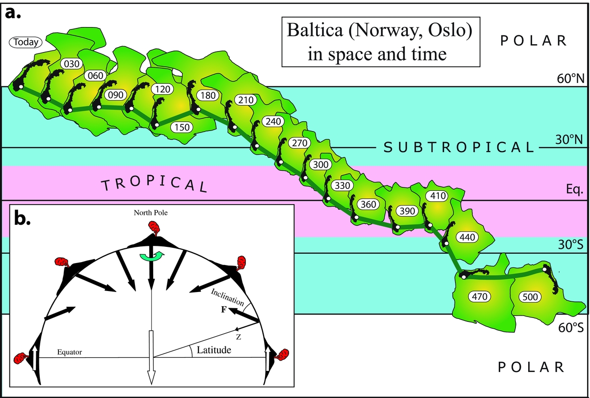
Figure 1. (a) The drift history for Baltica (Oslo) at 30 Ma intervals based on palaeomagnetic data listed in Torsvik et al. (Reference Torsvik, van der Voo and Preeden2012). (b) Magnetic field lines at the Earth's surface averaged over a sufficient time are equivalent to that expected from a geocentric axial dipole (GAD) aligned parallel to the Earth's rotation axis. At the Equator, the inclination is horizontal (zero) and at the North Pole the inclination is vertical (+90°). The remanent inclination recorded in rocks formed on the Earth's surface is dependent on the latitude [tan (Inclination) = 2×tan (Latitude)]. Volcanoes (caricatured) erupted in the northern hemisphere will acquire a thermoremanent magnetization upon cooling below a certain temperature (Curie temperature); the remanent inclination in the volcanoes will parallel the inclination of the Earth's field. Declinations in a normal polarity field, such as today's, should point to the north (GAD model). Longitude cannot be determined because volcanoes erupted at different longitudes will always have the same inclination and declination. F, total field intensity; Z, vertical field component.
The Early Palaeozoic is exceptional because practically all the continents were located in the southern hemisphere. Gondwana dominated the Early Palaeozoic Earth, but other important and separate continents, in addition to Baltica, included Laurentia (North America, Greenland, Scotland and NW Ireland) and Avalonia (including southern England) which were separated by wide oceans such as the Iapetus in the Early Ordovician. In Figure 2a we have reconstructed their location with palaeomagnetic data at 480 Ma, but at face value the relative longitudes between Baltica and the neighbouring continents of Laurentia, Gondwana and Avalonia are subjective, and commonly based on the rock record (opening and closure of oceans, orogenic events, zircon province, and more), and/or the distributions of fauna and flora: the latter indicating if continents or smaller terranes with similar biota were close to one another or were some way away (Torsvik & Cocks, Reference Torsvik and Cocks2017).
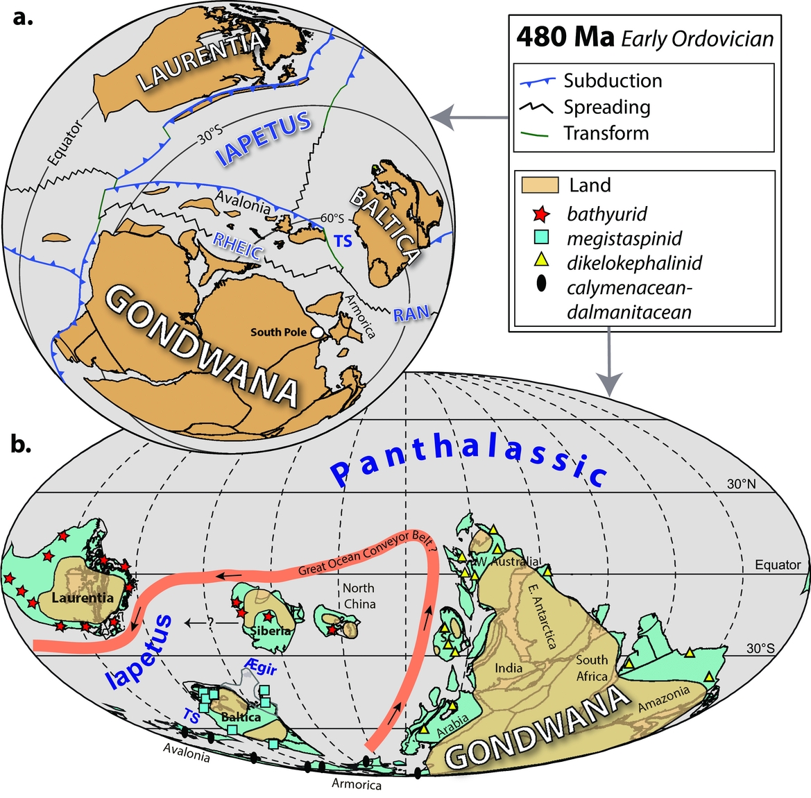
Figure 2. (a) Early Ordovician (480 Ma: Tremadocian) palaeomagnetic reconstruction of Baltica, Avalonia, Gondwana and Laurentia. Spreading centres, subduction zones, transform faults and some arc terranes are also shown (Domeier, Reference Domeier2015). (b) Early Ordovician (480 Ma) palaeomagnetic reconstruction as in (a) but on a global scale and also showing the emergent lands and the surrounding shallow shelf seas (coloured blue) preserved on today's continental lithosphere. Some of the principal sites of the four trilobite provinces are shown. The thick red line (with smaller black arrows) is a hypothetical ocean conveyor belt circulation scenario for the late Cambrian (Rasmussen et al. Reference Rasmussen, Ullmann and Jakobsen2016) but here adapted to our Early Ordovician reconstruction. SC, South China; TS, Tornquist Sea.
3. Faunal provinces and their distribution
The changing distributions of animals and plants through time have become better understood from the work of many generations of palaeontologists over more than 200 years. The factors which progressively separate those faunas and floras, giving them ecological space in which to evolve separately, are now well known. Some of the biota, particularly those plants whose seeds are transported widely by the wind, and plankton such as graptolites which were dispersed for long distances by ocean currents, are divided into provinces, which are of little help in establishing the distribution of old lands and seas. However, other biological groups are limited in their distributions within and between various continents, perhaps because they are or were shallow-marine benthos with short larval lives which cannot disperse quickly; perhaps because they have limited temperature ranges for successful breeding; and there is a variety of other factors which causes groups of genera, families and even orders to be identifiable as faunal or floral provinces relatively isolated from one another. Those provinces can help to identify separate land masses and continental shelf areas, and are particularly useful in deciphering the Palaeozoic, since they can often reflect differing palaeolongitudes, in contrast to palaeomagnetic studies, which only identify different palaeolatitudes. Of course the migration of those differing marine benthos was impeded either by land barriers or by seas and oceans too wide for their larvae to cross.
Depending on a variety of factors, such as the differences in temperatures between the poles and the Equator at different times, and the distances between the major continents, at some times faunal provinces were much more distinctive than at others. For example, in the Early Ordovician, four very distinctive provinces can be recognized in the shallow-shelf benthos (Fortey & Cocks, Reference Fortey and Cocks2003), including most trilobites and nearly all brachiopods. The first is the Mediterranean Province (often termed the Neseuretus or calymenacean–dalmanitacean Province by trilobite workers), which occupied the continental shelves around the higher latitudes of the massive continent of Gondwana (Fig. 2b). The second is the Baltic (or megistaspinid) Province, largely known from NW Europe (Baltica), which was at temperate southerly latitudes. The oceans in the lowest Equatorial latitudes hosted two distinct and separate faunal provinces: the bathyurid Province, which inhabited Laurentia, Siberia and North China, and a separate dikelokephalinid Province which colonized the seas surrounding the margins of the lower-latitude parts of Gondwana (which straddled the Equator). The presence of two different provinces at the same palaeolatitude indicates that the oceans separating Laurentia Siberia and North China (on the one hand) and that large sector of Gondwana (on the other hand) must have been large enough to have prevented the trilobite larvae from successfully crossing them, which enables us to conclude that those two continental masses must have been widely separated.
Our Early Ordovician reconstruction is well constrained in latitude due to the abundance of palaeomagnetic data; the width of the Iapetus Ocean varies between 4100 km (Laurentia–Avalonia) and 3700 km (Laurentia–Baltica), and c. 5000 km between Laurentia and Siberia. Because the bathyurid Province inhabited both Laurentia and Siberia, a narrower Iapetus Ocean (<1000 km) has been portrayed in many previous reconstructions (e.g. Torsvik et al. Reference Torsvik, Smethurst and Meert1996), often with Siberia located more westward and closer to Laurentia (black arrow with a question mark in Fig. 2b). But the distribution of that low-latitude warm fauna may also have been influenced by strong and persistent ocean currents (Fig. 2b). However, as we review below, there are other ways to calibrate potential continental longitudes in the Palaeozoic (the plume generation zone method, Section 7), but the Ordovician is not an ideal time for using that, due to limited occurrences of kimberlites. At c. 480 Ma, only North China is directly calibrated in longitude with kimberlites (485–474 Ma). Before (≥499 Ma) and after (≤462 Ma) that time, Laurentia and Gondwana were longitude-calibrated with kimberlites. Abundant kimberlites and a few large igneous provinces (LIPs) in Siberia only occur in the Late Ordovician and onwards (≤450 Ma).
After a period during the later parts of the Ordovician and nearly all the Silurian, significant faunal provincialization did not take place again until the Early Devonian (Emsian). By that time, the trilobites were less diverse, but in contrast the brachiopods had greatly radiated, so that the separate Emsian provinces are characterized by the brachiopods. During another greenhouse period in the Middle Permian, various brachiopod provinces were again well differentiated (Shi, Reference Shi2006), as shown in Figure 3. The Cimmerian Province was restricted to the more temperate latitudes up to 40°S in Sibumasu and NW India; and the Westralean Province to higher temperate latitudes above 50° in West Australia. In the northern hemisphere, the Sino-Mongolian–Japanese Province was restricted to a broader band of temperate palaeolatitudes in North China, some of the Mongolian terranes which made up the continent of Amuria, and only the northernmost of the island arcs now in Japan but then off South China (Fig. 3). The European Province was restricted to latitudes higher than 35°N, which extended over the Urals into the seaway which partly flooded the old Siberian Craton. But the Cathaysian Province, although named after the old word for China, is found in peri-Equatorial latitudes extending a very great distance from today's southern Europe across to many sites in Asia.
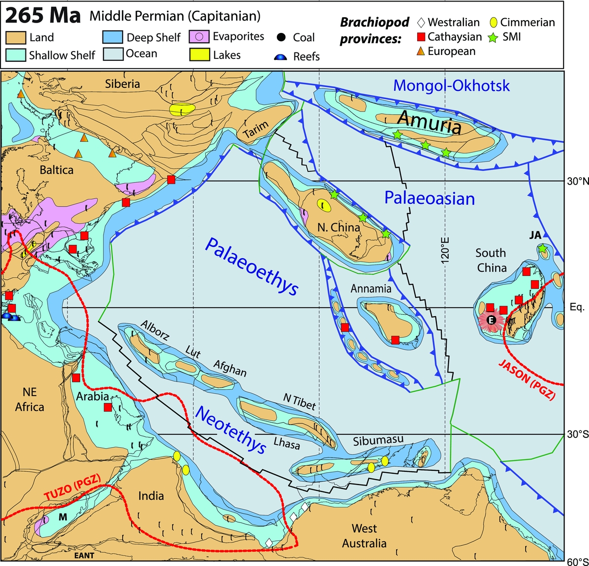
Figure 3. Permian palaeogeography of eastern Asia and adjacent areas (palaeomagnetic reconstruction), showing the extent of the dwindling Palaeotethys, the opening Neotethys, and the Palaeoasian and Mongol–Okhotsk oceans to the east of Pangaea and their surrounding continents, including South China (into which the Emeishan LIP was subsequently intruded at Equatorial latitudes at 260 Ma). As well as some of the sedimentary facies in the area, sites of some of the differing brachiopod faunal provinces are also plotted in the shallow shelf seas fringing the continents. Note also the flooded centre of the Siberian Craton and the first marine penetration into the area of Gondwana between NE Africa and India. Spreading centres (black), subduction zones (blue) and transform faults (green) are also shown (after Domeier & Torsvik, Reference Domeier and Torsvik2014; Torsvik & Cocks, Reference Torsvik and Cocks2017). JA, Japanese Arcs; SMI, Sino-Mongolian–Japanese Province.
4. Facies and glacial features
The distribution of latitude-sensitive and climate-dependent rock types (e.g. Scotese & Barrett in McKerrow & Scotese, Reference McKerrow and Scotese1990; Boucot, Xu & Scotese, Reference Boucot, Xu and Scotese2013) has proved useful in plate reconstructions, and, like fossils, can also have the advantage of being derived from rocks which have suffered tectonic activity, in contrast to palaeomagnetism where the original remanent magnetism is often overprinted (reset) by subsequent tectono-thermal events.
Glacial tillites are in general laid down in higher latitudes and are therefore useful in checking palaeomagnetic reconstructions during icehouse conditions with continental-scale glaciations, which occurred in the Late Ordovician, the Permo-Carboniferous (Fig. 4a) and the Plio-Pleistocene. However, dropstones deposited by icebergs must be treated with some caution since icebergs can be carried well down into temperate latitudes by ocean currents before they melt and drop their contained debris.
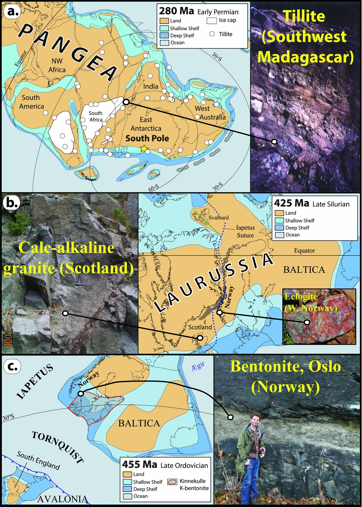
Figure 4. Examples of rocks useful in identifying local plate tectonic histories and thus assisting in palaeogeographical reconstructions or demonstrating latitudinal links between some major sediment types. (a) The Gondwana sector of Pangaea showing the contemporary pattern of lands and seas and higher-latitude glaciations during icehouse conditions in the Early Permian, with (right) glaciogenic Permian tillite in Madagascar. (b) Calc-alkaline granite (425 Ma) in Scotland (left) related to subduction and closure of the Iapetus Ocean (British Caledonide sector) which united Avalonia–Baltica and Laurentia in the Silurian to form Laurussia. The pattern of land and seas is also shown. Picture inset to the right is a Caledonian eclogite from western Norway. (c) Parts of Baltica and the approaching Avalonia (closure of the Tornquist Sea) at c. 455 Ma (Late Ordovician) showing the lands and seas but also the distribution of the extensive Kinnekulle Bentonite (right-hand picture) in SW Baltica (boundary with red lines). These came from volcanoes in England as the Tornquist Sea closed by subduction beneath Avalonia.
Carbonates are widespread throughout Phanerozoic rocks: they were largely laid down within tropical to subtropical latitudes, and thus their distribution can also be a useful check on the signals derived from palaeomagnetic and palaeontological analysis. Evaporites are most usually found in belts on either side of the Equator (the subtropics), and so their presence questions the reality of reconstructions which show them at high latitudes. Evaporites are distributed throughout the Phanerozoic, reconstructed evaporite sites average to subtropical latitudes of c. 31° (North or South) for the Cenozoic (Torsvik & Cocks, Reference Torsvik and Cocks2017), but mean evaporite latitudes became slightly lower backwards with time. That was caused by several arid periods with evaporites found at or near the Equator (e.g. in Central Pangaea in the Middle Permian, Fig. 3) but may partly also reflect the progressive slowing of Earth's rotation. A faster-spinning Earth displaces the subtropics equatorward and Christiansen & Stouge (Reference Christiansen and Stouge1999) have estimated that the subtropical high was displaced 5° towards the Equator in Ordovician times.
Coals can also help in the identification of old latitudes, since they are commonly confined to the Equator (wet conditions) or the northerly or southerly wet-belts at intermediate to high palaeolatitudes, as well demonstrated for the Middle Permian (Fig. 3). Coals indicate a prolonged excess of precipitation over evaporation, and occurrences show a pronounced peak (forest collapse) in the Late Carboniferous (~310 Ma), and smaller peaks in Late Permian, Mid Jurassic and Cenozoic times.
5. The rock record
Plate motions continuously reshape the surface of the Earth: mountains rise where plates converge and rifts open up where they move apart. Thus understanding and application of plate tectonic theory, integrated with Tuzo Wilson's (Reference Wilson1966) principles of its effect on rifting, crustal subsidence and ocean opening, subduction initiation and ocean closure, and finally continent–continent collision (the Wilson Cycle) are essential when modelling past geographies.
The waning stages of a Wilson Cycle involve oceanic subduction, closure and continental collisions which are recorded in the geological record, unless the rocks have been heavily reworked in younger events. For example, Avalonia rifted off the margin of Gondwana in the Early Ordovician (Fig. 2), and the later Avalonia–Baltica convergence history and Tornquist Sea closure are seen in faunal mixing and increased resemblance in palaeomagnetically determined palaeolatitudes for Avalonia and Baltica during Mid–Late Ordovician times (Torsvik & Rehnström, Reference Torsvik and Rehnström2003). By the Late Ordovician, Avalonia had drifted to palaeolatitudes comparable to those of Baltica (Fig. 4c, left-hand diagram), with subduction beneath Avalonia. That is clearly reflected in the geological record by Andean-type calc-alkaline magmatism in Avalonia (southern England), and explosive vents associated with that subduction were the source for gigantic Late Ordovician ash falls in Baltica (the Kinnekulle bentonite). The bentonite (Fig. 4c, right-hand picture) has a thickness of up to 2 m and extends for >1000 km in an E–W direction towards St Petersburg (Russia). Although the relative longitude (distance) between Baltica and Avalonia is not known in the Late Ordovician, they must have been relatively close, and Avalonia was also located south of the subtropical high and thus was in an ideal palaeo-position to supply Baltica with the large ash falls governed by westerly winds (Torsvik & Rehnström, Reference Torsvik and Rehnström2003).
The Caledonian Orogeny is a prime example of the final stage of a Wilson Cycle. Avalonia docked ‘softly’ with Baltica in the Late Ordovician but the combined land masses shortly thereafter collided much more powerfully with Laurentia during Silurian times (Fig. 4b, right-hand diagram). Subduction and continent–continent collision caused the calc-alkaline magmatism (Fig. 4b, left-hand picture) in Scotland / East Greenland and the ultra-high-pressure terranes in western Norway, which demonstrate subduction of Baltic continental crust beneath East Greenland to depths of 100 km or more (e.g. Andersen et al. Reference Andersen, Jamtveit, Dewey and Swensson1991). Those ultra-high-pressure terranes were subsequently exhumed rapidly during the Early Devonian.
Zircon forms the archive of continental crust since it is more stable than most other minerals, and U/Pb zircon ages most commonly reflect the crystallization age of the rock. U/Pb ages of detrital zircons can therefore be used to identify the provenance of the sedimentary particles, by comparing detrital zircon ages with crystallization ages of possible source rocks from the same, or another potential area for their origin. But perhaps the most serious challenge of using this method is the recurrent recycling of detrital zircons, which can homogenize material from diverse sources over a long period of time and great distances (Andersen, Kristoffersen & Elburg, Reference Andersen, Kristoffersen and Elburg2016). Thus the distribution of, for example, Mesoproterozoic South American zircon grains in European Ordovician rocks today does not unequivocally indicate how far apart the two original zircon sites were in the Palaeozoic.
6. Longitude calibration: the ‘zero-longitude’ Africa method
The relative positions of continents can be determined from ocean-floor magnetic anomalies and fracture-zone geometries since the Jurassic. The continents can subsequently be reconstructed objectively to their ancient positions on the globe in both latitude and longitude using the geometry and ages of hotspot volcanoes. But such reconstructions are only available since the Cretaceous (Fig. 5a). Conversely, palaeomagnetic reconstructions, which can be used for most of Earth's history, only constrain ancient latitudes (and rotations) and not continental longitudes. Such information, however, can be provided by choosing a global reference continent that has remained stable or quasi-stationary with respect to longitude (Burke & Torsvik, Reference Burke and Torsvik2004). Africa best meets that criterion, and other continents partnered in the same plate circuit will then occupy their own palaeolongitudinal positions. This is known as the ‘zero-longitude’ Africa method (Torsvik et al. Reference Torsvik, Müller, Van der Voo, Steinberger and Gaina2008a, Reference Torsvik, van der Voo and Preeden2012). Since the supercontinent of Pangaea began to form, the relative positions between many continents are reasonably well known, and palaeopoles from those continents are combined to a global apparent polar wander path (GAPWaP) in southern Africa coordinates. From the GAPWaP we first calculate Euler rotation poles for southern Africa, and the rotations for the remaining plates are then calculated by adding the relative plate motions to the ‘absolute’ rotations of southern Africa (Torsvik & Cocks, Reference Torsvik and Cocks2017). This reconstruction procedure originally led to the significant discovery that most reconstructed LIPs, and later also kimberlites (Torsvik et al. Reference Torsvik, Burke and Steinberger2010), were probably sourced from plumes near the edges of two Large Low Shear-wave Velocity Provinces in the lowermost mantle. These antipodal and near-Equatorial-centred provinces were named LLSVPs (Garnero, Lay & McNamara, Reference Garnero, Lay, McNamara, Foulger and Jordy2007) or more simply TUZO (beneath Africa) and JASON (beneath the Pacific) by Burke (Reference Burke2011).
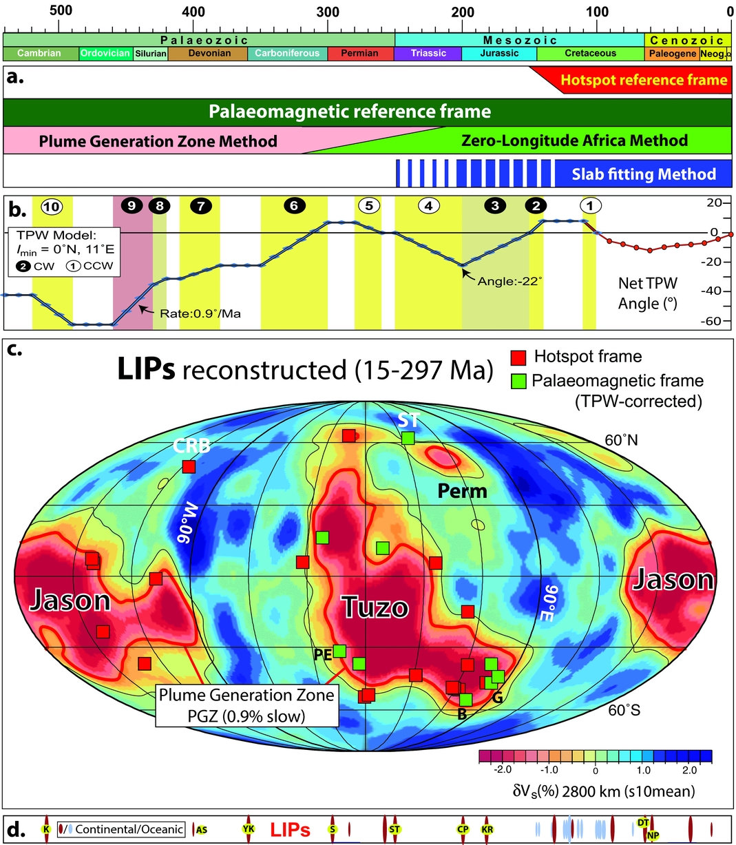
Figure 5. (a) Phanerozoic timescale and the various reconstruction frames/methods discussed in the text. A global moving hotspot is here used for the past 120 Ma, but the Pacific plate is reconstructed with a fixed hotspot frame back to 150 Ma (Doubrovine, Steinberger & Torsvik, Reference Doubrovine, Steinberger and Torsvik2012). The palaeomagnetic reference frame can be used for the entire Phanerozoic (and older times), the zero-longitude Africa method to calibrate palaeomagnetic longitudes is useful back to Pangaea formation (320 Ma), whilst the plume generation zone method to calibrate longitude is essential before 320 Ma but can also be used for younger times (Torsvik et al. Reference Torsvik, van der Voo and Doubrovine2014; Torsvik & Cocks, Reference Torsvik and Cocks2017). The slab-fitting method can be used back to the Early Mesozoic (depending on slab sinking times) but is perhaps most reliable after 130 Ma. (b) Net true polar wander (TPW) angle for the Phanerozoic (Torsvik et al. Reference Torsvik, van der Voo and Doubrovine2014). Net angle (deviation from the spin axis) is more than 60° in the Early Palaeozoic, but 22° maximum for Mesozoic–Cenozoic times. Ten phases of clockwise (CW) and counterclockwise (CCW) TPW rotations are identified from palaeomagnetic data between 540 and 100 Ma. TPW for the past 100 Ma calculated from a comparison of palaeomagnetic and hotspot reference frames (Doubrovine, Steinberger & Torsvik, Reference Doubrovine, Steinberger and Torsvik2012). (c) Reconstructed LIPs (15–297 Ma; table 1 in Doubrovine, Steinberger & Torsvik, Reference Doubrovine, Steinberger and Torsvik2016) draped on the s10mean tomography model where the plume generation zones (PGZs correspond to the 0.9% slow contour (Doubrovine, Steinberger & Torsvik, Reference Doubrovine, Steinberger and Torsvik2016). Most LIPs overlie the PGZs but the Columbia River Basalt (CRB) is anomalous because it is above a region of faster-than-average anomalies whilst the Siberian Traps (ST) overlie the smaller-anomaly PERM (Lekic et al. Reference Lekic, Cottar, Dziewonski and Romanowicz2012), which may be separate from JASON. Reconstructed LIPs which are also shown in Figure 7a are the 135–134 Ma Paraná–Etendeka (PE), the 132 Ma Bunbury LIP (B) and the 136 Ma Gascoyne LIP (G). (d) The ages of continental (red) and oceanic (blue) large igneous provinces (LIPs). Those LIPs younger than 300 Ma are reconstructed in (c), right-hand diagram. Note the larger number of oceanic LIPs after the Jurassic because the ocean floors have only been preserved from then on. LIP abbreviations are AS, Altai–Sayan; CP, Central Atlantic Magmatic Province (CAMP); DT, Deccan Traps; K, Kalkarindji; KR, Karroo; NP, North Atlantic Igneous Province; S, Skagerrak-centred LIP; ST, Siberian traps; YK, Yakutsk.
The ‘zero-longitude’ Africa method has also proved important for developing hybrid mantle frames Torsvik et al. Reference Torsvik, Müller, Van der Voo, Steinberger and Gaina(2008a) by combining hotspot and palaeomagnetic reconstruction frames. The first use of the ‘zero-longitude’ Africa method kept Africa fixed in longitude since Pangaea formed, but it is known from hotspot reference frames that Africa did move somewhat in longitude during and after the Late Cretaceous (black line in Fig. 6a). The workflow to build a hybrid reference frame back to Pangaea assembly is illustrated in Figure 6a, b. The palaeomagnetic section of the reference frame was calibrated in longitude (known movement in longitude of Africa) by the global mantle hotspot reference frame of Doubrovine, Steinberger & Torsvik (Reference Doubrovine, Steinberger and Torsvik2012). The palaeomagnetic reconstruction (Fig. 6b, PM) is remarkably similar to the global mantle hotspot reference frame reconstruction for Africa, apart from a c. 11° shift in longitude; that value is then used to correct all palaeomagnetic reconstructions before 120 Ma assuming zero-longitude motion of Africa. This is known as a global hybrid mantle reference frame, but the palaeomagnetic reconstructions before 120 Ma must also be corrected for true polar wander (TPW) because the palaeomagnetic reconstructions reference the continents to the Earth's spin axis and not the mantle.
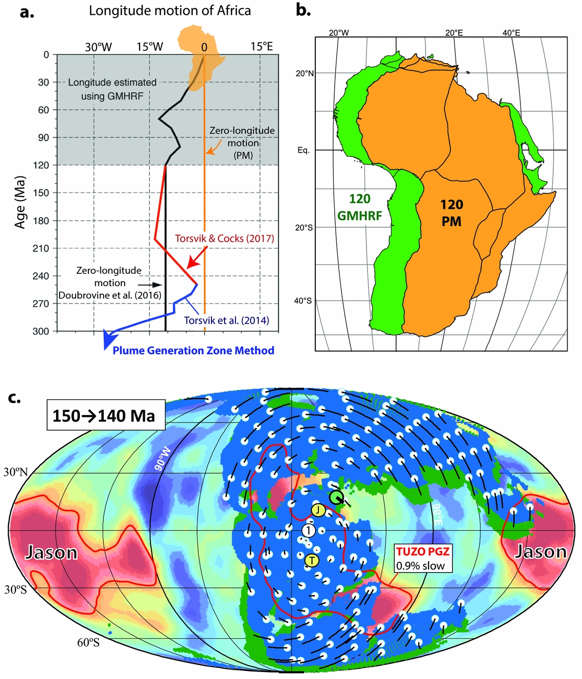
Figure 6. (a) Longitudinal motion of the African plate over the past 300 Ma used in Dubrovine et al. (2016; solid black line), Torsvik et al. (Reference Torsvik, van der Voo and Doubrovine2014; blue line for 250 Ma and older times), and Torsvik & Cocks (Reference Torsvik and Cocks2017; red line for between 250 and 120 Ma). (b) Example of reconstructing Africa at 120 Ma using the palaeomagnetic (PM) reference frame assuming zero longitudinal motion of Africa (Torsvik et al. Reference Torsvik, van der Voo and Preeden2012) and the global moving hotspot reference frame (GMHRF) of Doubrovine, Steinberger & Torsvik (Reference Doubrovine, Steinberger and Torsvik2012). The palaeomagnetic reconstruction is similar to the GMHRF reconstruction for Africa except for a ~11° shift in longitude that is used to correct all palaeomagnetic reconstructions before 120 Ma (assumed zero-longitude motion of Africa before that time). (c) TPW is determined by extracting the coherent (mean) rotation of all the continents in the palaeomagnetic reference frame, and such rotation around 11° at the Equator is recognized between 150 and 140 Ma (Torsvik et al. Reference Torsvik, van der Voo and Preeden2012). Total motions shown as black lines, connected to white dots (locations at the beginning of the time interval). Large green dot with thick black line indicates location and motion of the centre of mass of ‘all’ continents. Yellow dots (T and J) are the centre of mass for TUZO and the near-antipodal JASON LLSVPs. The red line is the 0.9% slow contour (plume generation zone, PGZ) in the s10mean tomography model (Doubrovine, Steinberger & Torsvik, Reference Doubrovine, Steinberger and Torsvik2016). Open white circle (marked 1) is the preferred centre for TPW (0°N, 11°E). Blue and green shading represent reconstruction at the start and at the end of the 150–140 Ma TPW episode.
TPW is determined by extracting the coherent mean rotation of all the continents (Fig. 6c) in the palaeomagnetic reference frame (Steinberger & Torsvik, Reference Steinberger and Torsvik2008; Torsvik et al. Reference Torsvik, van der Voo and Preeden2012). Since the Early Cretaceous, TPW can also be determined from a direct comparison of the palaeomagnetic and hotspot frames (e.g. Doubrovine, Steinberger & Torsvik, Reference Doubrovine, Steinberger and Torsvik2012). The net cumulative effect of TPW over the past 320 Ma (Fig. 5b) is relatively small (4.7±7.4°); the maximum deviation is c. 22° at c. 200 Ma, and is characterized by slow oscillations back and forth around approximately the same axis (0°N, 11°E), which is close to the LLSVP centres. LIPs for the past 300 Ma (Fig. 5c) were reconstructed with a global hybrid mantle reference where all LIPs older than 120 Ma (except those in the Pacific) are reconstructed with a TPW-corrected palaeomagnetic frame assuming zero-longitude motion before 120 Ma (black line in Fig. 6a). This hybrid mantle reference frame produces a remarkable correlation between reconstructed LIPs and the margins of TUZO and JASON (except the 15 Ma Columbia River Basalt), the so-called plume generation zones (PGZs; Burke et al. Reference Burke, Steinberger, Torsvik and Smethurst2008).
As an example of the global hybrid mantle reference frame at work, we show an Early Cretaceous (135 Ma) reconstruction. At that time, seafloor spreading in the Central Atlantic and the West Somali and Mozambique Basins was well under way. The Paraná–Etendeka LIP erupted at southerly subtropical latitudes, and contemporaneous LIPs in West Australia (132–136 Ma) and kimberlite (135±5 Ma) activity (South Africa, Namibia, NW Africa, and North America) appear to be sourced by plumes from the margin of TUZO (Fig. 7a). This is also exemplified in Figure 7b where we envisage that long-lived subduction along the South American margin was the triggering mechanism for a deep plume that eventually rose through the mantle and led to catastrophic upper mantle melting, forming the Paraná–Etendeka LIP (Svensen et al. 2017). In the Early Cretaceous, the Phoenix and Farallon plates bordered the South American margin, but considering the extremely long two-way mantle transit time (i.e. the time for a slab to sink from the surface to the core–mantle boundary plus the time for a plume to make the return trip), the initial subduction along the western margin of South Africa, which probably occurred 285–410 Ma ago, may have led to the plume that sourced the Paraná–Etendeka LIP.
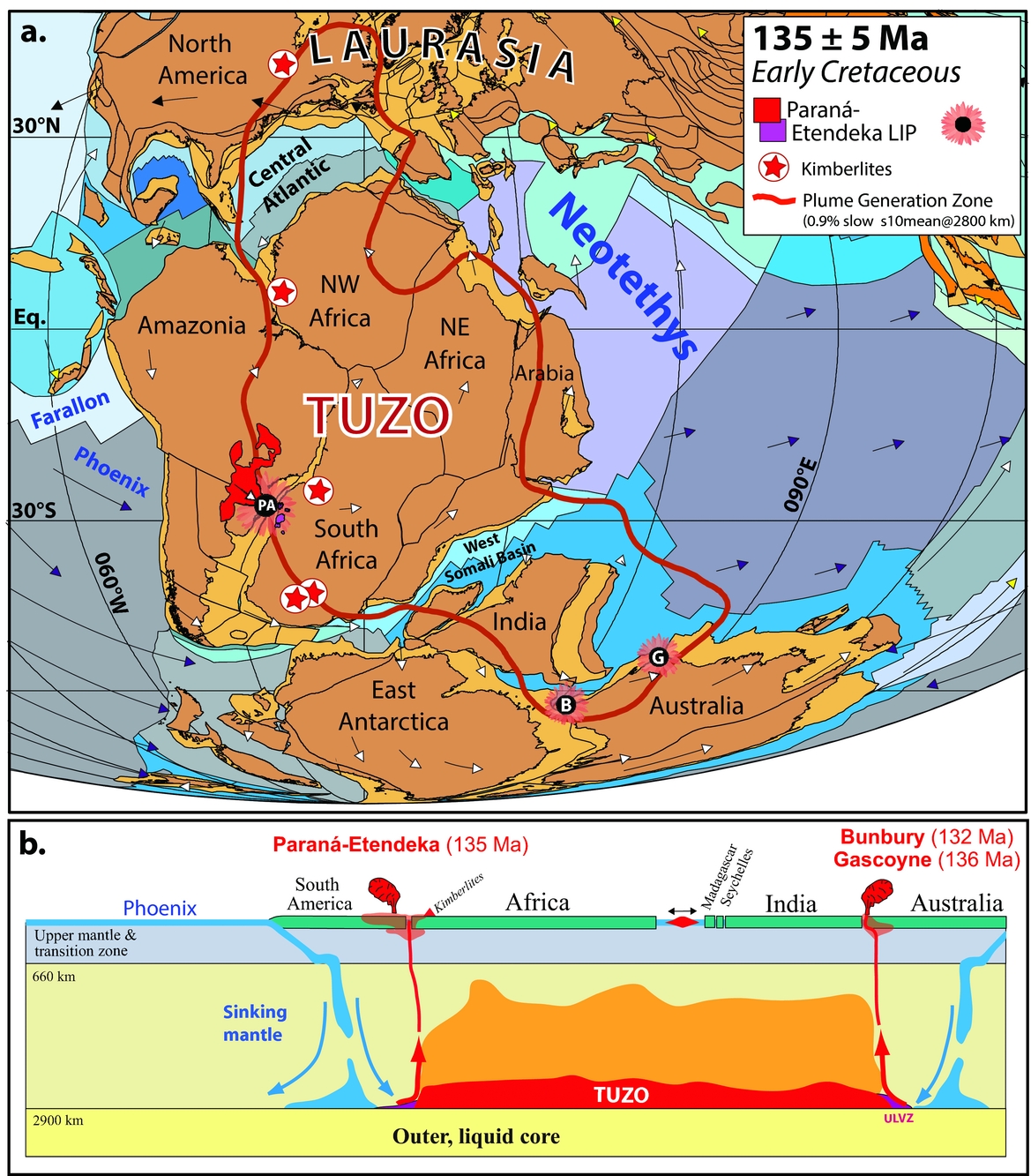
Figure 7. (a) Cretaceous (135 Ma) palaeomagnetic reconstruction and plate velocity vectors with the TUZO plume generation zone (thick red line) counter-rotated to account for TPW in order to relate reconstructed LIPs (135–134 Ma Paraná–Etendeka; 132 Ma Bunbury LIP; 136 Ma Gascoyne LIPs) and kimberlites (within ±5 Ma) to the deep mantle at the PGZ. (b) Subducted lithospheric slabs may interact with the margins of TUZO and JASON, triggering the formation of plumes. Cartoon profile approximately through the reconstructed Paraná–Etendeka LIP, North Madagascar – Seychelles, India and Australia at c. 135 Ma. Earth today is a degree-2 planet dominated by the two antipodal large low-shear-wave velocity provinces in the lower mantle beneath Africa (TUZO) and the Pacific (JASON), which are warmer but probably also denser and stiffer than the ambient mantle in its lowermost few hundred kilometres. Here we only show TUZO, and the orange colour is shown to indicate that the area above TUZO is also warmer than the background mantle. The triggering slabs for plumes sourcing the Paraná–Etendeka LIP and contemporaneous kimberlites in South Africa and Namibia were probably linked to subduction along the western margin of South America. The South Atlantic opened shortly after the Paraná–Etendeka LIP. Conversely, the Gascoyne and Bunbury LIPs were probably linked to old subduction systems along eastern Australia (see text). Oceanic plates (dynamic polygons) shaded in different colours are modified from Matthews et al. (Reference Matthews, Maloney, Zahirovic, Williams, Seton and Müller2016). ULVZ, Ultra Low Velocity Zone.
Paraná–Etendeka plume activity with volcanism started at 135–134 Ma, with large volumes of magma occurring in the first few million years which probably assisted the Cretaceous break-up of South America from Africa (Buiter & Torsvik, Reference Buiter and Torsvik2014) at c. 130 Ma. Comparably, the Gascoyne (136 Ma) and Bunbury (132 Ma) LIPs in West Australia (Fig. 7) may have assisted seafloor spreading between Australia–Antarctica and India. Separation of India from Australia–Antarctica probably started at ~136 Ma NW of Australia, and reached the southern tip of India at 130–126 Ma (Gibbons, Whittaker & Müller, Reference Gibbons, Whittaker and Müller2013).
7. Longitude calibration before Pangaea: the plume generation zone method
The remarkable correlation of reconstructed LIPs and kimberlites (e.g. Figs 5c, 7a) indicates the long-term stability of TUZO and JASON. Using that surface-to-core–mantle boundary correlation to locate continents in longitude, and a novel iterative approach for defining a palaeomagnetic reference frame corrected for TPW, Torsvik et al. (Reference Torsvik, van der Voo and Doubrovine2014) produced a model for absolute Palaeozoic plate motion with geologically plausible scenarios back to the Early Phanerozoic (540 Ma), with LIPs and kimberlites sourced from the margins of TUZO and JASON as in Mesozoic and Cenozoic times. The PGZ reconstruction method uses individual palaeopoles or APWPs from the various continents to reconstruct them in latitude and azimuthal orientation. However, in concert with geological information and the iterative approach for estimating TPW, we can construct realistic Palaeozoic maps by calibrating continental longitudes with their contained LIPs and kimberlites. Our Phanerozoic database now consists of nearly 1800 dated kimberlites, but almost 60% of these erupted in the Cretaceous (peaking at 80–90 Ma) and only 242 kimberlites and six LIPs are available for the Palaeozoic (Fig. 8). Palaeozoic kimberlites are found in six Palaeozoic continents, with notable peak occurrences in South Africa (Cambrian), Laurentia (Late Silurian – Devonian), and Siberia (Devonian–Carboniferous). There are low frequencies in the Ordovician (the only known kimberlite at c. 480 Ma in Fig. 2b is in North China) and in Carboniferous and Permian times.
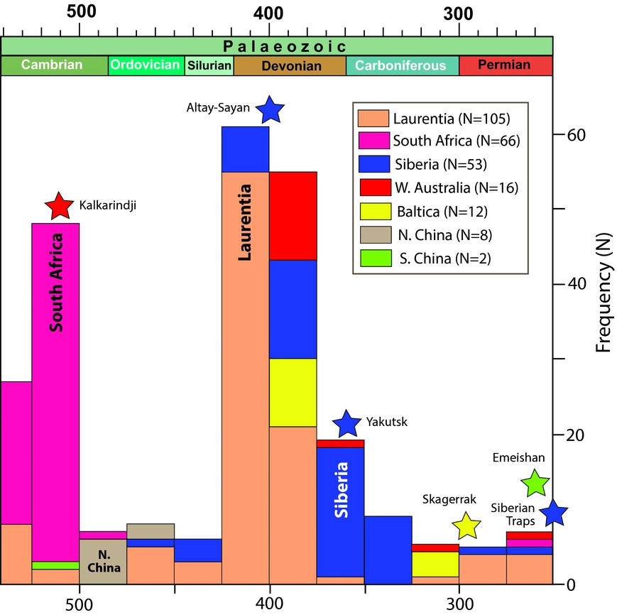
Figure 8. Frequency histogram showing the numbers of available dated kimberlites for the Palaeozoic (N=242) and LIPs that can be used to calibrate Palaeozoic longitudes for a total of six different continents. Laurentia, South Africa and Siberia have the highest frequencies of kimberlites, notably in Early–Mid Cambrian and Late Silurian to Early Carboniferous times (updated from Torsvik et al. Reference Torsvik, Burke and Steinberger2010).
As an example of the PGZ method, we show an Early Devonian reconstruction at 410 Ma, a time when abundant kimberlites are found in Siberia (Fig. 8), linked to TUZO, and in North America linked to JASON. At this time the bulk of the continents were assembled in Gondwana and Laurussia (Laurentia, Baltica and Avalonia), whilst Siberia and North China were separated from these superterranes by the Ægir, Rheic and Palaeotethys oceans. In the PGZ method, kimberlites and LIPs are fitted to the PGZ (thick red line in Fig. 9a) using TPW-corrected palaeomagnetic data. But Figure 9a is actually a palaeomagnetic reconstruction (related to the Earth's spin axis) and the TUZO and JASON PGZs are counter-rotated to account for TPW at this time.
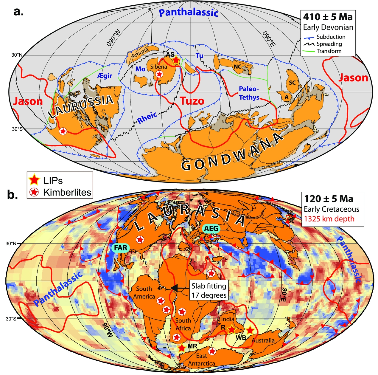
Figure 9. (a) Early Devonian palaeomagnetic plate reconstruction where Laurussian and Siberian kimberlites (410±5 Ma) have been used to calibrate their continental longitudes with the PGZ method. We also show the Altai–Sayan (AS) LIP that erupted 10 Ma later and is used to calibrate Siberia at that time (400 Ma). The PGZs of JASON and TUZU (red thick lines) have been counter-rotated to account for TPW. (b) Example of calibrating a 120 Ma reconstruction in longitude (van der Meer et al. Reference Van der Meer, Spakman and van Hinsbergen2010). A reasonable fit was obtained between a 1325 km tomographic depth-slice and the Farallon, and Tethys Ocean slabs when an absolute plate motion frame (Torsvik et al. Reference Torsvik, Burke and Steinberger2010) was shifted 17° westward. We also show how Indo-Atlantic 120±5 Ma LIPs and kimberlites (120±5 Ma) compare with the PGZ (thick red line). Interpreted subduction zones are shown in red. AEG, Aegean slab; A, Annamia; AS, Altai–Sayan LIP; FAR, Farallon slab; MR, Maud Rise LIP (125 Ma); Mo, Mongol–Okhotsk Ocean; R, Rajhmahal LIP (118 Ma); NC, North China; SC, South China; Tu, Turkestan Ocean; WB, Wallaby Plateau LIP (124 Ma).
A rather simple example of the PGZ reconstruction method is the positioning of South China in the Permian at c. 260 Ma when net TPW was zero. Pangaea did not include South China at any given time, which is therefore without longitudinal constraints, and in older maps has just been put in some arbitrary location east of Pangaea. The Emeishan LIP is on the South China block, and palaeomagnetic data position it at c. 4°S (Fig. 3). If the Emeishan LIP had erupted above a PGZ, there are several possible longitudinal locations where the line of latitude crossed the PGZ at eruption time. Pangaea covered TUZO, leaving only the options related to JASON, and the reconstruction with the Emeishan LIP above the western margin of Jason at ~134°E is the only realistic alternative (Torsvik et al. Reference Torsvik, Steinberger, Cocks and Burke2008b, Reference Torsvik, van der Voo and Doubrovine2014; Torsvik & Domeier, Reference Torsvik and Domeier2017). Since South China was one of the few independent continents at that time (most of the rest had combined to form Pangaea), the longitude-calibrated location of South China enables us to know the width of the intervening Palaeotethys Ocean between Pangaea and South China at 260 Ma, an invaluable data point for continental reconstructions (Fig. 3).
8. Calibrating longitude with subducted slabs (tomography)
Palaeomagnetic and hotspot reconstructions can also be tested or calibrated in longitude with the positions of subducted material (slabs) along convergent margins of the continents, which can be observed in tomographic models, and which van der Meer et al. (Reference Van der Meer, Spakman and van Hinsbergen2010) used to interpret the depth and timing of subduction for a total of 28 slab remnants in the mantle. Through correlation of those slabs with their surface geological record they determined a sinking rate of 12±3 mm a −1, which allowed global correlations of palaeo-subduction zones at the surface with seismic tomography images at depth. Those authors constrained the longitudes of ancient active margins as far back as the Permian by adjusting a global plate motion model based on palaeomagnetic data for improved fits with slab remnants in their tomographic model.
Figure 9b shows an example where all the continents in a global TPW-corrected palaeomagnetic reconstruction at 120 Ma were adjusted 17° westward so as to best fit the Farallon and Aegean Tethys slabs. The slab-fitting procedure in van der Meer et al. (Reference Van der Meer, Spakman and van Hinsbergen2010) is not strictly correct given that the longitude corrections should have been computed with an iterative TPW procedure (Torsvik et al. Reference Torsvik, van der Voo and Doubrovine2014), but this is perhaps trivial in comparison to the other uncertainties when computing a subduction reference frame. At 120 Ma, net TPW is rather small (c. 10°), but because all the continents are shifted westward the excellent correlation of Indo-Atlantic LIPs and kimberlites (120±5 Ma) with the PGZ (thick red line in Fig. 9b), as observed in a global mantle reference frame (hotspot frame), is somewhat poorer.
9. Orthoversion and pre-Pangaean longitudes
The PGZ reconstruction method uses an iterative approach for estimating TPW (Torsvik et al. Reference Torsvik, van der Voo and Doubrovine2014) which assumes that the location of the Earth's axis of minimum moment of inertia (I min) has remained similar in Phanerozoic times. Conversely, the Mitchell, Kilian & Evans (Reference Mitchell, Kilian and Evans2012) approach to determine pre-Pangaean palaeolongitude ─ dubbed the orthoversion model ─ assumes that Pangaea formed in a downwelling subduction belt which was orthogonal to the centroid of its supercontinent predecessor Rodinia (Evans, Reference Evans2003), and relies on TPW oscillations about mantle structures that shift longitude 90° for every supercontinent cycle. Mitchell, Kilian & Evans (Reference Mitchell, Kilian and Evans2012) therefore suggested that the Neoproterozoic (Rodinian) and Early Palaeozoic I min axis was located 90° away from the Pangaean I min axis.
Mitchell, Kilian & Evans (Reference Mitchell, Kilian and Evans2012) fitted great circles to Gondwana palaeomagnetic poles in South Africa coordinates to determine I min (i.e. pole to the great circle) relative to Gondwana, and in Late Ediacaran – Cambrian times (550–490 Ma) they observed that I min (30°S, 75°E) plotted near the West Australian / East Antarctica sectors of Gondwana (white star in Fig. 10a). Using 540–490 Ma mean poles for Gondwana and a slightly different geometry for Gondwana, we estimate I min at 50°S, 64°E (yellow star in Fig. 10a). Mitchell, Kilian & Evans (Reference Mitchell, Kilian and Evans2012) also fitted great circles to global Mesozoic poles in South African coordinates and estimated I min to 10°N, 001°E between 200 and 90 Ma (black star in Fig. 10a). The angular distance between their I min locations from 550–490 Ma and 200–90 Ma ─ in a South African (Gondwana) frame ─ is c. 81°, and they argued that the Pangaean I min was c. 90° different from the Gondwana (Rodinia) I min axis. Because Steinberger & Torsvik (Reference Steinberger and Torsvik2008) had argued for a mean I min of 10°E over the past 300 Ma, they suggested that the pre-Pangaean I min was located at 100°E (Fig. 10d). Episodes of TPW are assumed with the orthoversion method, but for the past 320 Ma we have only identified one long-lived episode where the GAPWaP in South African coordinates (Torsvik et al. Reference Torsvik, van der Voo and Preeden2012) is exclusively dominated by TPW, i.e. from 200 to 140 Ma (white boxes in Fig. 10a). Fitting a great circle to 200–140 Ma GAPWaP mean poles yields an I min (light brown star in Fig. 10a) of 8°N, 359°E (MAD=19°). Correcting the GAPWaP for TPW yield clustered mean poles (Fig. 10b) that confirm that the 200–140 Ma segment is indeed dominated by TPW (phases 3 and 2 with clockwise rotations in Fig. 5b; phase 2 in Fig. 6c).
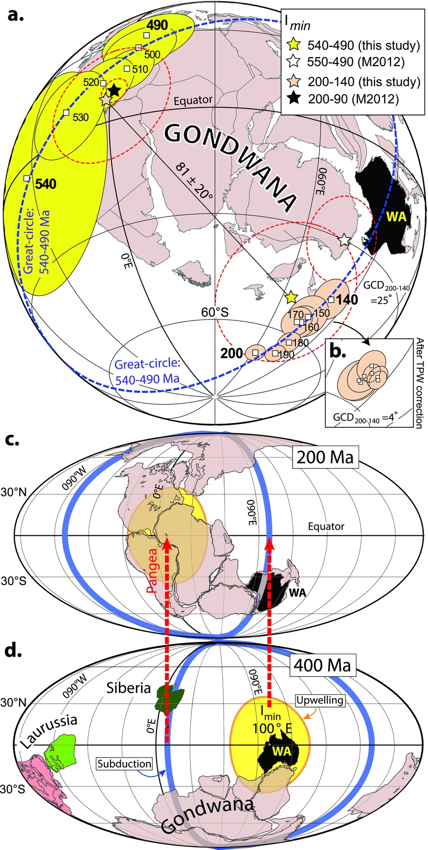
Figure 10. (a) Gondwana 540–490 Ma running mean poles in South African coordinates (Torsvik et al. Reference Torsvik, van der Voo and Preeden2012) shown with yellow A95 cones; I min (yellow star) with red stippled maximum angular deviation (MAD) angle is calculated as the pole to the great-circle (thick blue stippled line) fit of the mean-poles. This procedure (Mitchell, Kilian & Evans, Reference Mitchell, Kilian and Evans2012) assumes that the apparent polar motion between 540 and 490 Ma is exclusively a result of TPW. Similarly, Mesozoic GAPWaP running mean poles (200–140 Ma; Torsvik et al. Reference Torsvik, van der Voo and Preeden2012) are shown with light brown A95 cones (South African coordinates), the pole to the great-circle fit as thick blue stippled line, and I min is shown as a light brown star with red stippled MAD angle. The original I min estimated by Mitchell, Kilian & Evans (Reference Mitchell, Kilian and Evans2012, MReference Mitchell, Kilian and Evans2012) for 550–490 Ma (white star) and 200–90 Ma (black star) is shown for comparison. (b) GAPWaP running mean poles (200–140 Ma) shown after TPW correction (Torsvik et al. Reference Torsvik, van der Voo and Preeden2012, Reference Torsvik, van der Voo and Doubrovine2014). The great-circle distance is reduced from 25° to 4° and essentially all the mean poles statistically overlap, demonstrating that the 200–140 Ma segment of the GAPWaP (in the South African frame) is caused by TPW. (c, d) Palaeomagnetic reconstructions of Mitchell, Kilian & Evans (Reference Mitchell, Kilian and Evans2012) at 200 Ma and 400 Ma. Mitchell, Kilian & Evans (Reference Mitchell, Kilian and Evans2012) argue that for the past 260 Ma the I min was located at 0°, 10°E (Steinberger & Torsvik, Reference Steinberger and Torsvik2008), but, before that time, continents were calibrated in palaeolongitude such that the Rodinian/Gondwanan I min is ‘orthoverted’ at 0°N, 100°E. Yellow Equatorial circles represent ‘TUZO’, and the orthogonal thick blue great-circle swaths represent subduction girdles. In their 400 Ma reconstruction (d), Siberia is placed above the subduction girdle (downwelling) whilst we locate Siberia above the northwestern margin of TUZO (upwelling) due to abundant occurrence of kimberlites and one LIP at around this time (Figs 9a, 11f).
It is important to stress that Mitchell, Kilian & Evans (Reference Mitchell, Kilian and Evans2012) argue that I min has shifted c. 90° relative to Gondwana during the Palaeozoic whilst we move the continents relative to a fixed I min (Torsvik et al. Reference Torsvik, van der Voo and Doubrovine2014). The timing of this proposed migration occurred between 370 and 260 Ma (Mitchell, Kilian & Evans, Reference Mitchell, Kilian and Evans2012); this is portrayed with two of their reconstructions, one at 200 Ma (Fig. 10c, I min at 0°, 10°E) and another at 400 Ma (Fig. 10d) with I min at 100°E. Their global palaeomagnetic reconstructions, essentially ‘locking’ West Australia (controlling Gondwana) near 110°E (assumed I min longitude) from 500 to 370 Ma (Fig. 11b), can at times show similarities with ours, but Lower Palaeozoic longitudes differ markedly. As an example (Fig. 11a), Gondwana (West Australia) and Siberia differs by ~90° from our model (Fig. 11d) at c. 500 Ma whilst Laurentia has comparable longitudes.
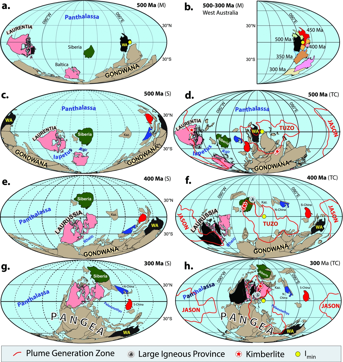
Figure 11. (a) 500 Ma (‘M’) reconstruction (Mitchell, Kilian & Evans, Reference Evans2013) for Gondwana, Baltica, Siberia and Laurentia. I min in this palaeomagnetic model is assumed to be at 0°, 100°E and Western Australia is essentially pinned in longitude to I min. (b) West Australia reconstructed in the Mitchell, Kilian & Evans (Reference Evans2013) model in 50 Ma steps from 500 to 300 Ma. (c–h) Palaeogeographic model comparisons at 500 Ma (Cambrian), 400 Ma (Devonian) and 300 Ma (Carboniferous–Permian boundary time). Left column (‘S’): palaeogeographical model of Scotese (Reference Scotese1997) and the dashed longitude meridians represent undetermined longitude. Right-hand column (‘TC’): palaeogeographical model of Torsvik et al. (Reference Torsvik, van der Voo and Doubrovine2014) and Torsvik & Cocks (Reference Torsvik and Cocks2017) (palaeomagnetic reference frame). Longitude is determined for those plates which host kimberlites or LIPs sourced from the plume generation zones (PGZ, thick red line) surrounding the TUZO and JASON LLSVP margins. The plotted kimberlites and LIPs are within ± 5 Ma for each reconstruction time, and we have counter-rotated the PGZs to account for TPW in order to relate the palaeomagnetic ‘surface’ reconstruction to the deep mantle. A, Altai–Sayan LIP (400 Ma); Kaz, Kazakhstania; S, Skagerrak Central LIP (297 Ma); WA, West Australia (shaded black). Those continents that eventually formed Laurussia in the Silurian are shaded pink (Laurentia, Baltica and Avalonia), Siberia is shaded green, whilst South and North China are shaded red and blue, respectively.
As with the other reconstruction methods, the orthoversion method has some clear shortcomings. First, determination of the I min axis by fitting great-circle segments to APWPs assumes that the apparent polar motion results exclusively from TPW. However, APWPs reflect the combined signal from both TPW and continental drift (plate motion), and for the past 300 Ma (Steinberger & Torsvik, Reference Steinberger and Torsvik2008; Torsvik et al. Reference Torsvik, van der Voo and Preeden2012) we only find one long-lived episode where TPW clearly dominates the APWP, i.e. between 200 and 140 Ma (Fig. 10a, b) Hence, the orthoversion method assumes TPW episodes (i.e. the dominance of TPW signal) to estimate I min, in contrast with estimating I min by kinematic inversion techniques (Steinberger & Torsvik, Reference Steinberger and Torsvik2008; Torsvik et al. Reference Torsvik, van der Voo and Preeden2012). Second, the orthoversion method only determines I min relative to a continent (e.g. South Africa in Fig. 10a) which is subsequently displaced by younger plate motions and TPW episodes. Thus I min cannot be recovered to its original location in the absolute palaeogeographic sense and its longitude has to be postulated a priori based on the conceptual orthoversion model (90° shifts between successive supercontinent cycles) and considerations of absolute plate velocities.
10. Discussion and future challenges
Palaeomagnetism is undoubtedly the most useful pre-Cretaceous tool in placing the previous positions of now detached portions of the Earth's lithosphere. At face value, longitudes are unknown in palaeomagnetic reconstructions, but with the ‘zero-longitude’ Africa motion approach we can derive semi-absolute reconstructions. This approach probably works best after Pangaea break-up from 200 Ma, but can theoretically be used back to Pangaea assembly (320 Ma), and can be combined with hotspot reconstructions to produce a hybrid mantle frame, which can be tested or calibrated with the slab-fitting method. With all the reconstruction methods, there are also many sources of potential error in developing subduction reference frames, and since the first pioneering global model of van der Meer et al. (Reference Van der Meer, Spakman and van Hinsbergen2010) the age of several slabs has been reinterpreted (e.g., van der Meer, van Hinsbergen & Spakman, Reference Van der Meer, van Hinsbergen and Spakman2017), there has been major revision of ocean closures, e.g. Mongol–Okhotsk Ocean (Van der Voo et al. Reference Van der Voo, van Hinsbergen, Domeier, Spakman, Torsvik, Anderson, Didenko, Johnson, Khanchuk and MacDonald2015), and also development of more complex subduction models, e.g. along the western margin of North America (Sigloch & Mihalynuk, Reference Sigloch and Mihalynuk2013) and in the north Pacific (Domeier et al. Reference Domeier, Shephard, Jakob, Gaina, Doubrovine and Torsvik2017). Future subduction reference frames must also be computed using an iterative TPW scheme.
Before Pangaea, we can use the PGZ reconstruction method, but there are rather few LIPs and kimberlites, and pre-Pangaean geographies must be constructed in close concert with known geological and tectonic constraints (Sections 3–5). A highly multidisciplinary approach is required, and using full-plate models, which define the entire system of lithospheric plates (including the largely synthetic oceanic lithosphere), ensures kinematic continuity. Such models are now routinely constructed in GPlates (Boyden et al. Reference Boyden, Müller, Gurnis, Torsvik, Clark, Keller and Baru2011) using dynamic polygons (e.g. Figs 2a, 3, 7a and 9a) which self-close at any arbitrary spatial or temporal scale (Gurnis et al. Reference Gurnis, Turner and Zahirovic2012), making the models functionally seamless in time and space.
The PGZ reconstruction method assumes TUZO/ JASON stability, a degree-2 Earth and TPW must be estimated in an iterative manner. The method clearly depends on how the PGZs are defined, which correspond to the areas with the largest lateral gradients of the shear-wave velocity directly above the core–mantle boundary (Torsvik et al. Reference Torsvik, Smethurst, Burke and Steinberger2006), and thus depend on the choice of seismic tomography model. The differences between most tomography models of the deepest mantle, however, are typically small. We have extensively used the 1% slow-velocity contour (thick red lines in Figs 9 and 11) in the lowermost layer of the mean shear-wave tomographic model SMEAN (Becker & Boschi, Reference Becker and Boschi2002) to define the PGZ. More recently we have used the s10mean model (Doubrovine, Steinberger & Torsvik, Reference Doubrovine, Steinberger and Torsvik2016) which is similar to SMEAN, but the PGZ in this model is approximated by the 0.9% slow contour (thick red line in Figs 6c, 7a).
Mitchell, Kilian & Evans (Reference Mitchell, Kilian and Evans2012) argue that pre-Pangaean ‘absolute’ longitudes can be estimated with the orthoversion method. But their reconstructions are reported in a palaeomagnetic reference frame, i.e. determined with respect to the spin-axis rather than the mantle. They did not estimate TPW ─ only estimated the location of the I min axis ─ and it is thus not possible from that paper to put their reconstructions into a mantle reference frame to compare the fits of LIPs and kimberlites.
We have extensively used the PGZ method to identify absolute plate motions before Pangaea in a quantitative manner. But if TUZO and JASON were highly mobile ─ or Earth alternated between degree-2 and degree-1 modes (e.g. Zhong et al. Reference Zhong, Zhang, Li and Roberts2007; Li & Zhong, Reference Li and Zhong2009; Zhang et al. Reference Zhang, Zhong, Leng and Li2010) ─ then this method is invalidated and we have no means for calibrating longitude and to derive absolute reconstructions before Pangaea (a geodynamic dead end). The latest default rotation engine in GPlates (Matthews et al. Reference Matthews, Maloney, Zahirovic, Williams, Seton and Müller2016) and ours use the PGZ reconstruction method for the Palaeozoic (Torsvik et al. Reference Torsvik, van der Voo and Doubrovine2014; Torsvik & Cocks, Reference Torsvik and Cocks2017) but should be used with caution if the assumptions for the PGZ method are found to be unsound. Our digital plate rotation model is available in both mantle (combination of global moving hotspot and TPW-corrected palaeomagnetic reference frames) and palaeomagnetic frames, but we stress that the mantle reference frame is only to be used when attempting to relate surface and deep mantle processes (e.g. Fig. 5c). Conversely, climate modelling or reconstructions of climatically sensitive sedimentary data or fauna demands a palaeomagnetic reference frame as input. In order to also relate deep mantle processes to surface processes in the palaeomagnetic reference frame, one can simply counter-rotate the PGZs to account for TPW (red lines in Figs 2, 7a, 9a, 11d, f, h). This way, one can perceive how the surface distribution of, for example, LIPs and kimberlites relates to the deep mantle, and at the same time plot climatically sensitive sedimentary data that should not be corrected for TPW. Global plate reconstructions and continental outlines in GPlates (Boyden et al. Reference Boyden, Müller, Gurnis, Torsvik, Clark, Keller and Baru2011) format (www.gplates.org) can be downloaded at www.earthdynamics.org/EarthHistory/.
Maps showing the distribution of old lands and seas have been constructed for over 100 years; their sophistication has constantly evolved and hopefully for the better. In more recent times, Christopher Scotese and his associate authors have constructed highly cited global maps of all periods throughout the Phanerozoic based on palaeomagnetic, palaeontological and sedimentary data (e.g. Scotese, Reference Scotese1997). It is instructive to compare some of those reconstructions (Fig. 11c–h) with those we have made using the added longitude information through the PGZ reconstruction method. The two sets have much in common, but the contrast between them is particularly vivid for the Palaeozoic. As an example, at 500 Ma we position Laurentia c. 80° west of the Scotese model, West Australia (part of Gondwana) differs 165° in longitude, whilst we locate Siberia 80° west of the Scotese model (Fig. 11c, d). Both reconstructions also differ substantially from that of Mitchell, Kilian & Evans (Reference Mitchell, Kilian and Evans2012) and notably their location of West Australia / Gondwana (Fig. 11a; see Section 9). At 400 Ma, the longitudes for Laurentia and West Australia (Gondwana) differ by 85° and 30°, respectively (Fig. 11e, f). Conversely, the 300 Ma reconstructions are much more similar in longitude (Fig. 11g, h).
We are well aware of the shortcomings of the Phanerozoic maps which have been published, many by ourselves, and it is also perhaps unrealistic today to construct truly meaningful palaeogeographical maps for the Precambrian. That is partly because there are no Precambrian floral or faunal provinces: even though the Late Precambrian Ediacara Fauna shallow marine faunas (which include several different animal phyla) are widespread, they show no sign of any provincialization (McCall, Reference McCall2006). However, this is chiefly because a progressively larger proportion of older rocks have been subsequently tectonized, not only obliterating primary magnetic signatures, but also making realistic reconstruction of the original margins and overall sizes of all the original terranes progressively more difficult in those older rocks. The supercontinent Rodinia, which probably existed over most of the Neoproterozoic from ~1000 to 700 Ma, has been recognized by many palaeogeographers (e.g. Li et al. Reference Li, Bogdanova and Collins2008; Li, Evans & Murphy, Reference Li, Evans and Murphy2016; Evans, Reference Evans2013; Meert, Reference Meert2014), but the details of its continental make-up are debated. Reconstructing Rodinia with confidence and the subsequent transition to the great Gondwana terrane is particularly challenging because palaeomagnetic data, notably from the Ediacaran (635–541 Ma) and the Early Cambrian, are sparse, unreliable and sometimes outright contradictory!
Acknowledgements
The Research Council of Norway, through its Centres of Excellence funding scheme, project number 223272 (CEED), is acknowledged for financial support. We thank Mat Domeier, Pavel Doubrovine and Bernhard Steinberger for helpful comments, and David Evans and Conall Mac Niocaill for constructive reviews.


