


Introduction
The planktonic larvae of benthic marine invertebrates and fish, collectively the meroplankton, are the only dispersing life-history stage for the colonization of new habitats for many species and are of critical importance in determining the level of population connectivity and gene-flow (e.g. Allcock & Strugnell Reference Allcock and Strugnell2012). In general, the Antarctic meroplankton community has been poorly studied; in part due to the remote location and its associated logistic challenges, as well as the general acceptance of Thorson's Rule that pelagic larval stages were less common in polar environments where low temperatures and scarcity of food would favour species with different developmental strategies (Mileikovsky Reference Mileikovsky1971). Thorson's Rule has been increasingly questioned and its full validity has been limited to some taxa, regions or geological times (Poulin et al. Reference Poulin, Palma and Féral2002, Laptikhovsky Reference Laptikhovsky2006).
Despite the number of Antarctic species with a planktonic life stage being smaller than in other environments (Poulin et al. Reference Poulin, Palma and Féral2002), it is noticeable that the most conspicuous and abundant taxa in many Antarctic benthic assemblages, such as the sea urchin Sterechinus neumayeri (Meissner), the starfish Odontaster validus (Koehler), the ophiuroid Ophionotus victoriae Bell and the scallop Adamussium colbecki (Smith), have a planktonic dispersal stage (Poulin et al. Reference Poulin, Palma and Féral2002 and references therein). Further, there is now considerable evidence that larvae are abundant in Antarctic coastal environments, both on the Antarctic Peninsula and in the Ross Sea (Stanwell-Smith et al. Reference Stanwell-Smith, Peck, Clarke, Murray and Todd1999, Absher et al. Reference Absher, Boehs, Feijó and da Cruz2003, Freire et al. Reference Freire, Absher, Cruz-Kaled, Kern and Elbers2006, Sewell Reference Sewell2006, Thornhill et al. Reference Thornhill, Mahon, Norenburg and Halanych2008, Bowden et al. Reference Bowden, Clarke and Peck2009, Sewell & Jury Reference Sewell and Jury2009, Reference Sewell and Jury2011).
However, few studies have examined the meroplankton community of Antarctic oceanic waters, with only three studies in the Antarctic Peninsula region (Shreeve & Peck Reference Shreeve and Peck1995, Vázquez et al. Reference Vázquez, Ameneiro, Putzeys, Gordo and Sangrà2007, Ameneiro et al. Reference Ameneiro, Mouriño-Carballido, Parapar and Vázquez2012). Recent genetic studies have shown a high degree of connectivity in some marine invertebrates, with populations from the Antarctic Peninsula and the coastal waters of the Ross Sea shelf (more than 5000 km apart) sharing the same mitochondrial haplotypes (e.g. Wilson et al. Reference Wilson, Schrödl and Halanych2009). This pattern is shown in species with one or two dominant haplotypes and a circum-Antarctic distribution, likely to have found refugia during the Last Glacial Maximum (LGM) within shelf habitats (e.g. the sea urchin S. neumayeri, the decapod Chorismus antarcticus (Pfeffer) and the nemertean Parborlasia corrugatus (McIntosh)) or in deeper waters (e.g. the decapod Nematocarcinus lanceopes Bate and the echinoderms Astrotoma agassizii Lyman and Odontaster validus) (see review in Allcock & Strugnell Reference Allcock and Strugnell2012). If this broad-scale population connectivity is occurring as a result of larval dispersal (Allcock & Strugnell Reference Allcock and Strugnell2012), we might hypothesize that larvae are dispersed between the Antarctic Peninsula and the Ross Sea via the clockwise Antarctic circumpolar current (ACC), and might be present in the oceanic waters beyond the Ross Sea shelf.
As part of the New Zealand International Polar Year - Census of Antarctic Marine Life (IPY-CAML) voyage to the Ross Sea (Hanchet et al. Reference Hanchet, Mitchell, Bowden, Clark, Hall and O'Driscoll2008, Pakhomov et al. Reference Pakhomov, Hall, Williams, Hunt and Stevens2011, Safi et al. Reference Safi, Robinson, Hall, Schwarz and Maas2012), meroplankton samples were collected in three different oceanic waters: above the Ross Sea shelf, the Ross Sea slope and in the oceanic offshore waters to the north of the Ross Sea near Scott Island and the Admiralty Seamount. Using a combined morphological/molecular approach (Heimeier et al. Reference Heimeier, Lavery and Sewell2010), we describe the diversity and abundance of these meroplankton communities during the late summer, with three aims: i) to identify how meroplankton diversity, abundance and species composition varies across regions, depth ranges and water masses (with distinct physical and chemical characteristics), ii) to obtain a better understanding of the influence of environmental variables on the meroplankton distribution in oceanic waters, and iii) to examine relationships between meroplankton and the benthic species composition (from the literature and online databases), looking for putative benthic sources for the larvae found in the water column.
Methods
Sample collection
Samples were collected during the IPY-CAML voyage to the Ross Sea by the RV Tangaroa between 12 February and 11 March 2008. Meroplankton tows were performed at 13 stations (Fig. 1, Table I) with a Multi Opening/Closing Net and Environment Sensing System (MOCNESS-1), equipped with a 1 m2 rectangular frame and 200 μm mesh, as described in detail in Pakhomov et al. (Reference Pakhomov, Hall, Williams, Hunt and Stevens2011). Three regions of the Ross Sea were sampled: i) the Ross Sea shelf, ii) the Ross Sea slope, and iii) the offshore Antarctic waters to the north of the Ross Sea, adjacent to the Admiralty Seamount and Scott Island, and under the influence of the ACC (see Fig. 1). MOCNESS-1 allows samples from different depth ranges to be collected on each tow, and between four and five different depth strata (from nearly bottom to surface) were sampled at each station (total of 53 samples). Two whole water column samples (from bottom to surface) were also collected at stations 156 and 158. After collection, each plankton sample was divided using a Folsom splitter. A representative subsample was fixed in 4% buffered formaldehyde and kept as a reference sample, while an equivalent subsample (25–6.25% of the original sample) was preserved in 70% ethanol and used in our meroplankton studies. Depth profiles of temperature, salinity and chlorophyll a were estimated using CTD casts (described in Pakhomov et al. Reference Pakhomov, Hall, Williams, Hunt and Stevens2011) and/or the sensors equipped in the MOCNESS gear at all stations (except for station 168 where data from the nearest station (143) from Hanchet et al. (Reference Hanchet, Mitchell, Bowden, Clark, Hall and O'Driscoll2008, p. 166) has been used). Water samples were collected at all stations at different depths using Niskin bottles to assess levels of dissolved nutrients, particulate carbon and nitrogen, dissolved reactive phosphorus and pigments, including size fractioned chlorophyll a and phaeopigments (Safi et al. Reference Safi, Robinson, Hall, Schwarz and Maas2012, Chang et al. Reference Chang, Williams, Schwarz, Hall, Maas and Stewart2013).

Fig. 1 Position of the MOCNESS sampling stations covered in the IPY-CAML voyage to the Ross Sea. Stations 42, 57 and 95 were located over the Ross Sea shelf, stations 122, 156, 158, 168 and 170 over the slope and stations 194, 232, 238, 261 and 283 on the offshore Antarctic. Continuous line represents the Ross Sea shelf break at a depth of 750 m.
Table I Meroplankton samples collected in the Ross Sea and adjacent waters during the IPY-CAML voyage of February–March 2008.

No MOCNESS samples were collected at station 42 from 0–200 m or at station 283 from 2370 m to the sea floor. MOCNESS sampled strata in which no larvae were found are shown in bold. Samples from which a flow measurement was not obtained are shown in italics.
Water masses were defined as in Pakhomov et al. (Reference Pakhomov, Hall, Williams, Hunt and Stevens2011).
ASW = Antarctic Surface Water, BW = Antarctic Bottom Water, CDW = Circumpolar Deep Water, SW = shelf water.
In the laboratory, meroplankton samples were sorted in a standard Bogorov tray under a dissecting microscope and the samples were assigned to morphological operational taxonomic units (OTUs) following the methods previously used in coastal Ross Sea research (Sewell Reference Sewell2006, Sewell & Jury Reference Sewell and Jury2011). Each larva was then rinsed and stored in 70% ethanol in a single well of 96-well PCR plates for further DNA-based analysis, as described in Heimeier et al. (Reference Heimeier, Lavery and Sewell2010).
Genetic analysis
DNA identification was attempted on representative specimens from each morphological OTU from each sample. DNA extraction was performed on these larvae using a Proteinase K-Chelex protocol as described in Heimeier et al. (Reference Heimeier, Lavery and Sewell2010), and between 0.5–2 μl of the resulting solution was used as template in Polymerase Chain Reaction (PCR) amplification of up to three loci (partial fragments of the 16S rRNA and cytochrome c oxidase subunit I (COI) genes from the mitochondrial genome and the 18S rRNA gene from the nuclear genome). PCR master mixes were magnesium chloride (MgCl2) 2.5 mM, PCR Buffer 1X, 0.25 μM of each primer, 0.2 mM of each dNTP and included 0.25 Units of Taq Polymerase (Invitrogen) in a 20 μl reaction volume. The complete set of primers and slight variations in the PCR annealing temperatures are described in Supplementary Table 1 (which will be found at http://dx.doi.org/10.1017/S0954102013000795). Primers were tailed at the 5’ end with M13 sequences (M13F 5’-TGTAAAACGACGGCCAGT-3’ and M13R 5’-CAGGAAACAGCTATGAC-3’) for ease of sequencing. PCR profiles consisted of an initial denaturation at 94°C for 3 minutes, followed by 35–40 cycles of 30 seconds of denaturation, 60 seconds of annealing and 60 seconds of 72°C extension, and a final extension of 3 minutes at 72°C. PCR amplifications of fragments of the desired length were checked on 1.6% agarose gels. Purified PCR products were sequenced using either M13F or M13R primers with the BigDye®Terminator kit and analysed on an ABI 3130 automated capillary sequencer (ABI 3130; Applied Biosystems).
Sequences were trimmed by removing PCR primers and bases with an error probability higher than 0.05, analysed and compared using Geneious (downloadable from www.geneious.com), and a molecular identification of the sequences was obtained following the methods described in Heimeier et al. (Reference Heimeier, Lavery and Sewell2010). Sequences from each locus were analysed separately, and one alignment per phylum or class was constructed for each locus. Each alignment consisted of query sequences, homologous sequences downloaded from the National Center for Biotechnology Information (NCBI) database and reference sequences obtained in this study from specimens identified by taxonomists from New Zealand's National Institute for Water and Atmospheric Research (NIWA) invertebrate collection. Alignments were constructed using MAFFT (multiple alignment using fast Fourier transform; Katoh et al. Reference Katoh, Misawa, Kuma and Miyata2002) within Geneious and edited by eye, and the best model of nucleotide substitution was chosen with modelgenerator (Keane et al. Reference Keane, Creevey, Pentony, Naughton and McInerney2006) using the Akaike information criteria. Maximum likelihood trees were then generated using PHYML (Guindon & Gascuel Reference Guindon and Gascuel2003) as implemented in Geneious with the specifications suggested by modelgenerator. The resulting trees were edited using FigTree v1.3.1 (http://tree.bio.ed.ac.uk/software/figtree/) and resolved independently. For each tree, an identification label was given to a cluster of query sequences based on the bootstrap support of this cluster and on the presence of reference sequences within it. COI sequences were also identified using the Barcode of Life identification tool (http://v3.boldsystems.org/) which can provide a match using sequences that are not yet publicly available. A final identification was given to a sample by combining the information from the three trees (when available) using the criteria specified in Heimeier et al. (Reference Heimeier, Lavery and Sewell2010). Sequences obtained from larval specimens identifying OTUs and from the NIWA invertebrate collection have been uploaded to Genbank with accession numbers KF713373–KF713484. Reference sequences used in the identification process can be found in the supplementary material.
A new occurrence table for each sample was generated using the molecular OTUs (mOTUs) obtained (summarized in Table II). Alpha diversity was estimated for each sample using the Shannon-Wiener diversity index. No correlation was found between larval abundance or Shannon-Wiener diversity index and the volume of water filtered in each sample (-0.059 and -0.375, respectively), suggesting that water volume was not a confounding factor in our univariate analyses (for detailed information on water volumes filtered per sample see Supplementary Table 2, http://dx.doi.org/10.1017/S0954102013000795).
Table II Summary of the molecular operational taxonomical units (mOTUs) found in the Ross Sea during the IPY-CAML voyage.

mOTUs that were only represented by one or two specimens have been excluded (see text for details).
N = number of specimens, Ab = abundance of each mOTU in each region expressed as mean ± standard error per 100 m3, < 200 = percentage of specimens from each mOTU in each region found above the 200 m mark.
Average (mean ± standard error) abundance per water mass for each mOTU was calculated for Antarctic Bottom Water (BW), Antarctic Surface Water (ASW), Circumpolar Deep Water (CDW) and shelf water (SW).
Statistical analysis
Three factors that might influence the distribution and abundance of the meroplankton in the oceanic Ross Sea were examined in our univariate and multivariate analyses:
-
i) Region = shelf, slope, offshore Antarctic waters.
-
ii) Depth = samples collected above and below 200 m depth (samples that crossed the 200 m boundary were not included).
-
iii) Water masses as defined by Pakhomov et al. (Reference Pakhomov, Hall, Williams, Hunt and Stevens2011) = shelf water (SW), Antarctic Surface Water (ASW), Circumpolar Deep Water (CDW) and Antarctic Bottom Water (BW) (samples that traversed water mass boundaries were labelled as mixed (Table I) and were not included).
The latter factor is obviously confounded with both region and depth, as not all water masses occurred at each sampling station and the water masses are restricted to certain depth ranges in the Ross Sea (e.g. SW occurs only on the Ross Sea shelf, and ASW and BW occur only at the surface and bottom depths, respectively).
Our approach, therefore, in analysing the diversity, abundance and species composition of the meroplankton was a conservative one. For the univariate analyses (larval abundance and Shannon-Wiener index), we first performed a linear mixed regression model with the restricted maximum likelihood (REML) method for an unbalanced design with the factors region and depth using the R software environment (http://www.r-project.org/) with the functions lm and ANOVA from the statistics package (v2.15.2) and pairwise Tukey's honestly significance difference tests from the agricolae package (v1.1-3). We then explored the influence of water masses on the unexplained variation by including this as an additional factor in the analysis. Due to the confounding factors discussed above, we conducted two linear regression analyses: the first with region and depth as the first-tested terms, and the second with water mass being the factor accounted for first.
Multivariate analysis of the mOTUs identified in the meroplankton community was performed using PRIMER-E 6.1.11 (Plymouth Marine Laboratory) software with the PERMANOVA+ add-on. Meroplankton abundances (specimens per 100 m3) were transformed (square root) before the calculation of a Bray–Curtis similarity matrix between samples. This transformation was chosen to lessen the impact of high abundance taxa but after checking the Spearman correlation values between original and transformed matrices. Stations lacking flow measurements (station 158 and the uppermost samples from stations 232 and 283) were not included in this analysis.
Changes in the meroplankton community were visualized using a non-metric multidimensional scaling (MDS) plot. A Euclidean distance matrix between samples was constructed using 14 normalized environmental variables (the full list can be seen in Supplementary Table 2, http://dx.doi.org/10.1017/S0954102013000795) and the BIO-ENV procedure in PRIMER-E was used to estimate the combination of environmental variables best explaining the biological matrix. We allowed up to five environmental variables to be combined in order to get the highest correlation between environmental and biological matrices. The global test under the BIO-ENV procedure looked for the significance of that correlation by performing 9999 permutations of the sample labels and calculating the number of cases in which a higher correlation was found.
Permutational analysis of variance (three-way PERMANOVA) was used to test for differences between samples from different regions, depths and water masses. As with the univariate analyses, we conducted two PERMANOVA tests: the first with region and depth as the first-tested terms, and the second with water mass being the factor accounted for first. This approach allowed us to test for any effect of the water masses that cannot be attributed to differences in region or depth. The PERMANOVA used 99 999 permutations of residuals under a reduced model and Type I sum of squares. Pairwise PERMANOVA tests were performed between levels of those factors identified as a significant source of variation by the main test using 99 999 permutations of raw data and Type I sum of squares. The PERMDISP test was run to assess differences in the dispersal of the samples from their group centroid (levels of region, depth or water mass), using 99 999 permutations of least-squares residuals. To further discriminate between groups of samples found to be significantly different in the PERMANOVA procedure, a canonical analysis of principal coordinates (CAP) was performed, producing a constrained ordination for each factor (region, depth and water mass). Furthermore, CAP provided a permutation test to examine differences between levels of each factor, and a cross-validation test in which the success of the allocation of a sample in the correct group can be used as a proxy of the distinctiveness of the meroplankton community in that group. To distinguish which mOTUs were contributing to the multivariate patterns, the similarity percentages (SIMPER) procedure was performed within PRIMER-E.
Results
Morphological sorting of 55 samples from the 13 stations resulted in over 21 000 individuals initially identified as larvae. This figure does not include copepod nauplii or euphasiid larvae, as these were morphologically identified as holoplankton during the sorting process. DNA sequences revealed, however, that the majority of initially-identified larvae were actually holoplanktonic species and these were removed from further analyses. Examples included the pelagic polychaete Pelagobia longicirrata Greeff (180 specimens), early developmental stages of the pteropods Limacina helicina (Phipps) (15 193 specimens) and Clione limacina (Phipps) (84 specimens) or small ostracods (130 specimens). A total of 408 sequences from three loci helped us identify 36 meroplankton mOTUs comprising 825 specimens; no larvae were found in 11 of the 55 samples (20%).
Meroplankton diversity
A total of 36 mOTUs from eight phyla were identified in the meroplankton community from the oceanic Ross Sea (Table II):
Phylum Annelida (13 mOTUs) - annelids were represented by early stages (trochophore, metatrochophore) and nectochaetes from at least seven families of polychaetes (Spionidae, Orbinidae, Chaetopteridae, Polynoidae, Amphinomidae, Nephtidae and Phyllodocidae). Three mOTUs were represented by only a single specimen: Aurospio sp. (station 158, 480–300 m), Amphinomidae sp. (station 42, 400–200 m) and Nephtidae sp. (station 95, 210–105 m), and the only two specimens of the Orbinidae mOTU were collected in the same sample (station 156, 600–780 m).
The taxonomy of Antarctic polyonids has recently been under revision, and it has been noted that ‘it was currently not possible to definitely identify specimens which had been pre-identified as Polynoe thouarellicola Hartmann-Schröder, Polyeunoa laevis McIntosh or Polynoe antarctica Kinberg due to the confused situation in the literature’ (Barnich et al. Reference Barnich, Gambi and Fiege2012). For statistical analysis, we considered two mOTUs within this family: Polyeunoa-Antarctinoe spp. and Polynoidae sp. Analysis of the 18S locus supported these two clades, although the mtDNA analysis showed that one of these clades, the Polyeunoa-Antarctinoe mOTU, could include representatives of up to five different species from at least two genera. Reference sequences obtained from positively identified specimens of Polyeunoa laevis, along with a positive match from Antarctinoe ferox (Baird) on the BOLD identification engine were used to match sequences from this clade and therefore name this multi-genera mOTU.
Phylum Echinodermata (seven mOTUs) - echinoderms from three classes were found in the oceanic waters of the Ross Sea: Asteriodea (five specimens of Odontasteridae sp.) and Holothuroidea (three mOTUs) larvae were only found on the Ross Sea shelf, whereas the Ophiuroidea (three different species) appeared in both shelf and slope samples. Two of the Holothurian mOTUs, Elasipodida sp. and Synaptidae sp., were only found once, at stations 42 (750–600 m) and 95 (210–105 m).
Phylum Mollusca (four mOTUs) - four gastropods molluscs were distinguished using molecular markers, including three different Littorinimorpha mOTUs and the nudibranch Tergipes antarcticus Pelseneer. Gastropods were present in all three regions, but only T. antarcticus veligers were found in the offshore Antarctic waters (stations 261 and 283, near Scott Island, Fig. 1). Three of the mOTUs were present only in samples above 200 m depth, and only the Littorinimorpha spp. mOTU was found in samples between 200 and 400 m depth from the Ross Sea shelf.
Phylum Arthropoda (four mOTUs) - crustaceans were represented by barnacle nauplii from two different species (the Antarctic acorn barnacle Bathylasma corolliforme (Hoek) and an unknown Verrucidae, found only once at station 158) and the pelagic stages of two species of benthic shrimps (N. lanceopes and a Pasiphaeoidea species). Greater taxonomic resolution could not be determined in the latter case due to the low resolution of the 18S locus and the lack of reference sequences from the only known Pasiphaeoidea from the Southern Ocean, Pasiphaea scotiae (Stebbing).
Phylum Chordata (four mOTUs) - larvae from four fish species were found in the oceanic Ross Sea. Pleuragramma antarctica Boulenger was only found in shelf waters, Bathylagus antarcticus Günther on the slope, and Electrona antarctica Günther and Magnisudis cf. prionosa (Rofen) were restricted to the offshore Antarctic waters. Identification of M. cf. prionosa is partially tentative, molecular markers place them as a close relative of M. atlantica (Krøyer) the only representative of that genus with sequences available, and M. cf. prionosa is the only species of this genus present in Antarctica (data from www.iobis.org and the Australian Antarctic Division data centre https:/data.aad.gov.au/).
Phylum Cnidaria (two mOTUs) - although six mOTUs were identified, these were collapsed into two different OTUs (Hexacorallia spp. and Hydrozoa spp.) due to the low resolution of the 18S locus.
Other phyla (two mOTUs) - a single specimen of a Bdelloid Rotifer (we were unable to identify it to a species level due to the poor coverage in public databases for this phylum) was found at station 261. A single OTU included all Palaeonemertea spp. (Phylum Nemertea) specimens, which shared the same 18S sequence but formed two 16S clusters. No COI sequences were obtained from these mOTUs.
Meroplankton distribution in the Ross Sea
Meroplankton samples collected on the Ross Sea shelf were dominated by annelids, gastropods and echinoderms, with more than 90% of all echinoderms found in shelf waters (Fig. 2). The Ross Sea slope was dominated by crustacean larvae, primarily barnacle nauplii, and annelids that accounted for nearly 30% of the slope meroplankton. The dominant phyla in the samples from the offshore Antarctic waters were molluscs and nemerteans (Fig. 2), which were concentrated in the upper layers of the water column, with 100% of the molluscs (T. antarcticus) and 93% of the nemertean larvae found above 200 m depth (Table II). Polychaete diversity in the offshore Antarctic was the lowest of all regions, with only three mOTUs present in these samples.
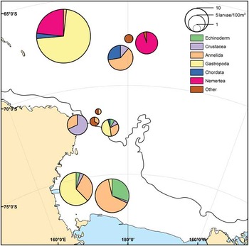
Fig. 2 Meroplankton composition in the Ross Sea, showing the contribution of each major taxa per sample. Pie radius represents overall larval abundance, expressed in specimens per 100 m3. Stations not fully sampled (42) or lacking flow measurements (156 and 283) were not represented. Continuous line represents the Ross Sea shelf break at a depth of 750 m.
Overall, meroplankton density was 5.19 larvae per 100 m3 and the median abundance of larvae in a sample was 3.35 larvae per 100 m3. The maximum value recorded was 246.15 larvae per 100 m3 in the uppermost (surface to 100 m depth) sample from the offshore station 261 (Fig. 1). Whereas no larvae were found in 11 samples, eight of those samples were in the offshore region (Table I). A linear mixed regression model using REML showed that overall meroplankton density was significantly higher (between 3 times and 33 times depending on the region) in the upper 200 m of the water column (P = 0.012) but showed no significant differences between the three regions (P = 0.37) (Table III). Difference in larval abundance between water masses were non-significant (P = 0.061) after accounting for all the variation attributed to region and depth (Table III). These differences between water masses became significant when this factor was the first term tested (P < 0.001), but the Tukey's test found significant differences only between ASW (limited to the first 100 m of the water column) and both SW and CDW (usually below 200 m depth); revealing the confounding effect of water mass and depth (ASW–SW difference = 49.21, P = 0.043 and ASW–CDW difference = 58.78, P = 0.005).
Table III Larval abundance (specimens per 100 m3) and Shannon-Wiener diversity index of the meroplankton community in different regions, depths and water masses.

In a & b number of samples in each category is shown in parentheses.
Probabilities shown in bold represent significant values P < 0.05.
ASW = Antarctic Surface Water, BW = Bottom Water, CDW = Circumpolar Deep Water, df = degrees of freedom, SW = shelf water.
Meroplankton samples containing just one mOTU (11 samples from slope and offshore Antarctic regions) had a value of zero for the Shannon-Wiener index. Maximum values of this index were found in samples from the shelf (station 42, 200–400 m, H’ = 1.61 and station 95, 210–315 m, H’ = 1.63) and offshore Antarctic waters (station 283, 200–800 m, H’ = 1.56). A linear mixed regression model using REML showed significant differences in Shannon-Wiener index between regions (P < 0.001), but not between depths above and below the 200 m mark (P = 0.15) (Table III). The pairwise Tukey's test showed a significantly higher Shannon-Wiener index on the shelf than on both slope (difference = 0.69, P = 0.001) and offshore (difference = 0.723, P = 0.002), but not between slope and offshore (difference = 0.032, P = 0.978). We could not detect a significant (P = 0.6) influence of the different water masses on meroplankton diversity that was not accounted for by region and depth (Table III). The linear mixed regression model showed significance of water masses when this factor was tested for first, revealing the confounding effect between water mass and region.
Overall, the influence of the confounding factors changes between univariate measures of larval abundance and diversity. For larval abundance, the water masses that are significantly different are those that are restricted to certain depths (ASW vs SW, CDW), perhaps due to differences in physical and chemical factors (e.g. temperature, salinity, pressure). In contrast, for larval diversity, the water masses that are significantly different (Tukey < 0.05) are those that are restricted to certain regions, between SW (which is restricted to the Ross Sea shelf) and CDW (absent from the shelf) a similar pattern to that observed in the regional analysis (SW–CDW difference = 0.74, P = 0.0018). Based on this study, we suggest that larval abundance in the oceanic Ross Sea is strongly linked with depth, regardless of water mass, and that, similarly, larval diversity is linked to region, likely due to the diversity of the underlying benthos.
Multivariate analysis
The dataset used in the multivariate analysis consisted of 586 larvae from 36 mOTUs found at those stations from which a flow measurement was obtained (39 samples, Table I). A highly dissimilar meroplankton community was found in the oceanic waters of the Ross Sea, with PERMANOVA analyses showing significant differences with both region and depth. Confounding effects of these factors and the different water masses present in the Ross Sea made it impossible to detect any influence of the water masses that was not accounted for by the other two factors. Comparison of the meroplankton community (Bray–Curtis similarity matrix) with the environmental variables (Euclidean distance matrix) using the BIO-ENV procedure revealed a low correlation between both matrices. The highest Spearman correlation value was obtained with a combination of median temperature, depth and latitude (0.456) and those results were shown to be significant in a permutation test (P < 0.0001). (Full results are shown in Supplementary Table 2, http://dx.doi.org/10.1017/S0954102013000795).
Multivariate analysis supported the differences revealed with the Shannon-Wiener index and the larval abundance. The MDS plot showed regional clustering (Fig. 3a), with shelf and offshore samples comprising two clusters and samples from the Ross Sea slope occupying an apparently broader space in the plot; although the PERMDISP procedure did not reveal any difference in the dispersion from the group centroid between regions (P = 0.5715). Differences between samples from different depth ranges (above and below 200 m depth) were not obvious in the MDS plot (Fig. 3a), with only a central cluster formed by samples from above 200 m depth, and a non-significant PERMDISP test (P = 0.188).

Fig. 3 Multidimensional scaling (MDS) plots for meroplankton samples, based on a square root transformed Bray-Curtis similarity matrix. Samples are labelled according to the a. coastal to oceanic gradient and depth or b. water mass affecting them. ASW = Antarctic Surface Water, BW = Antarctic Bottom Water, CDW = Circumpolar Deep Water, SW = shelf water.
Differences in the meroplankton community between water masses were also shown on the MDS plot (Fig. 3b), with CDW and SW samples constituting two distinct clusters. PERMDISP showed a significant (P = 0.0017) difference in the dispersion from the centroid between groups; although significant pairwise differences were not found between ASW, SW and CDW (P > 0.1), only between BW and the other three water masses (ASW: P = 0.035, SW: P = 0.014 and CDW: P < 0.01).
The PERMANOVA test found significant differences between samples from different regions and depth ranges but not between water masses (Table IV). The interaction term between region and depth was also significant, which is evidence for a different effect of depth in each region, where a different pool of species is present. Differences between water masses became significant when the order of terms in the PERMANOVA test was altered, supporting the confounding effect between water mass and the other two terms shown previously in the univariate analysis. Pairwise PERMANOVA tests returned significant differences between all three regions studied and between depth ranges, but only differences between SW and CDW and between ASW and CDW were found to be significant (Monte Carlo p values did not find differences between the pairs with few unique permutations) (Table IV).
Table IV a. Main permutational analysis of variance (three-way PERMANOVA) of meroplankton samples from different regions, depth ranges and affected by different water masses. b. Pairwise PERMANOVA tests between samples from different regions, depths and water masses. For those water mass pairs for which only a small number of unique permutations were possible, Monte Carlo p values were calculated.

Statistically significant differences are noted in bold.
df = degrees of freedom, SS = sum of squares, MS = mean sum of squares, P(perm) = p value calculated through permutation, Unique perms = number of unique permutations, P(MC) = p value calculated using Monte Carlo sampling.
ASW = Antarctic Surface Water, BW = Antarctic Bottom Water, CDW = Circumpolar Deep Water, SW = shelf water.
Canonical ordination analysis showed a clear discrimination of samples according to the three factors studied (Fig. 4). Permutation analysis in the CAP procedure gave support to all three sources of variation (region, depth and water masses), which were accounted for independently (Table V). Cross-validation tests performed gave depth the highest overall allocation success with 88.24%. Allocation success in the regional analysis had an overall 79.41% rate and all allocation errors were between adjacent regions, which gave additional support to the regional and depth influence. Although the differences between water masses were found significant by the CAP permutation test, their cross validation showed a lower allocation success (67.64%), and all ASW samples (the only water mass present in all three regions) were incorrectly assigned to different water masses, showing the lack of group distinctiveness of the meroplankton community within this water mass.

Fig. 4 Constrained ordination (canonical analysis of principal coordinates, CAP) plots for meroplankton samples, based on a square root transformed Bray–Curtis similarity matrix. a. Analysis using eight principal coordinates analysis (PCO) axes to maximize the percentage of correct cross-validation test for the region factor. b. Depth factor analysis using 21 PCO axes. c. Water mass factor analysis using 22 PCO axes. δ = correlations for CAP axes, ASW = Antarctic Surface Water, BW = Antarctic Bottom Water, CDW = Circumpolar Deep Water, SW = shelf water.
Table V Summary of the canonical analysis of principal coordinates (CAP) for factors region, depth and water mass. Rows indicate original (true) sample groups and columns the identity assigned by the allocation procedure.
m = number of principal coordinates analysis (PCO) axes selected by maximizing the allocation success, CAP1–3 = correlation enclosed on the CAP axis, misclassification = percentage of the samples allocated in a different group in the cross-validation procedure with the errors disclosed below.
ASW = Antarctic Surface Water, BW = Antarctic Bottom Water, CDW = Circumpolar Deep Water, SW = shelf water.
SIMPER analysis showed low average similarities between samples from the same region, depth range or water mass. Within group similarities were particularly low for the offshore Antarctic (10.19%, Supplementary Table 3 http://dx.doi.org/10.1017/S0954102013000795), which might be a result of the larger geographical distances between sampling stations (Scott Island stations 194, 232 and 238, and Admiralty Seamount stations 261 and 283 are more than 400 km apart) and/or the extremes in bathymetry between stations, with bottom depths ranging from c. 400 m (stations 194, 238 and 261) to > 3000 m (stations 232 and 283).
Similarities between samples from the shelf were also low (15.8%), and potential drivers of this lack of similarity can be found in the distance between stations (between c. 120 km and 300 km). Low similarities between slope samples (15.3%) are likely to be due to the different oceanographic and sediment characteristics found in this region, with stations 122, 156 and 158 located over the shelf break and stations 168 and 170 having an oceanographic profile similar to the offshore stations (Supplementary Table 3 http://dx.doi.org/10.1017/S0954102013000795). Shelf meroplankton similarities were mainly driven by the two polynoid mOTUs, the cucumarid holothurian and Littorinimorpha gastropods. The slope meroplankton was best characterized by the Hexacorallia OTUs, the Antarctic acorn barnacle B. corolliforme and a Laonice sp. polychaete. The Phyllodocinae sp. mOTU, the myctophid fish E. antarctica and nemertean larvae (Palaeonemertea spp.) accounted for most of the similarity within offshore samples (Table VI, full results in Supplementary Table 3 http://dx.doi.org/10.1017/S0954102013000795).
Table VI Summary of the SIMPER analysis between samples from different Ross Sea regions, showing the species contributing most to the similarities within regions and dissimilarities between them. Stars denote the contribution of each species: **** = more than 20%, *** = between 10–20%, ** = between 5–10%, * = less than 5%. Full results can be found in Supplementary Table 3.

Dissimilarities between the two most geographically distant regions (Ross Sea shelf and offshore Antarctic) reached almost 100% with only two mOTUs (Polychaetes Spiophanes sp. and Phyllodocidae sp.) occurring in both areas. These two are the only mOTUs occurring in samples from all three sampling regions. Dissimilarities between adjacent regions were generally smaller but above 90% (Table VI). Dissimilarity between shelf and slope samples were mainly driven by three mOTUs: the acorn barnacle B. corolliforme, Littorinimorpha spp. and Polyeunoa-Antarctinoe spp. The B. corolliforme larvae were more abundant on the slope, whereas the polynoids and gastropods were found in greater numbers in the shelf samples. Two other species contributing to the differences between these two regions were the two Laonice clades: Laonice sp. B was only found in shelf samples, whereas Laonice sp. A appeared in both slope and offshore Antarctic regions (Table VI).
Dissimilarities between the offshore Antarctic and the Ross Sea slope were driven mainly by B. corolliforme, Hexacorallia and Phyllodocinae sp. mOTUs. Species dominating the offshore Antarctic meroplankton community (Palaeonemertea spp. and T. antarcticus) also contributed to the dissimilarities between these two regions (Table VI).
A SIMPER analysis between samples from different depth ranges showed even smaller within group similarities, 8.37% between samples from below 200 m depth and 11.88% between samples from above 200 m. They were driven mainly by the Hexacorallia spp. mOTU between deeper samples, while the acorn barnacle B. corolliforme and the Laonice sp. A mOTU were more important between the samples from above 200 m depth (Table VII, Supplementary Table 4 http://dx.doi.org/10.1017/S0954102013000795).
Table VII Summary of the SIMPER analysis between samples from above and below 200 m depth, showing the species contributing most to similarities within depth group and dissimilarities between above and below 200 m depth. Stars denote the contribution of each species: **** = more than 20%, *** = between 10–20%, ** = between 5–10%, * = less than 5%. Full results can be found in Supplementary Table 4.

The pattern observed with the SIMPER analysis between water masses reflected that of the regional and depth analysis. Water masses restricted to a particular region (SW) reflected the similarities shown in the regional analysis (c. 15% within group similarity driven by Polyeunoa-Antarctinoe spp., Littorinimorpha spp. and Cucumariidae sp. mOTUs), whereas those water masses restricted to a particular depth range (ASW and CDW) showed the low similarities seen in the depth analysis, due to the same mOTUs (ASW was 7.7% mainly due to the presence of B. corolliforme as in the upper 200 m group and CDW was 12.38% driven by the Hexacorallia spp. Phyllodocinae sp. and Laonice sp. A mOTUs). A summary of this SIMPER analysis is shown in Table VIII, and a comprehensive table showing the percentage contribution can be found in the Supplementary Table 5 http://dx.doi.org/10.1017/S0954102013000795.
Table VIII Summary of the SIMPER analysis between samples from different water masses, showing the species contributing most to similarities within water masses and dissimilarities between significantly different groups. Stars note the contribution of each species: **** = more than 20%, *** = between 10–20%, ** = between 5–10%, * = less than 5%. Full results can be found in Supplementary Table 5.

ASW = Antarctic Surface Water, BW = Antarctic Bottom Water, CDW = Circumpolar Deep Water, SW = shelf water.
Discussion
Oceanic samples collected during the IPY-CAML voyage to the Ross Sea have revealed a diverse meroplankton community, which shows significant differences between different regions (shelf, slope and offshore Antarctic) and depth ranges, and a weak, although significant, correlation with the measured environmental variables (latitude, median water temperature and depth). Differences in the meroplankton communities between sampling locations were due to not only the presence or absence of certain taxa, but also a result of changes in OTU abundance.
Abundance of meroplankton is undoubtedly linked to depth. The uppermost samples, from the first 200 m of the water column, contained nearly twice the specimens than samples from below that mark (332 larvae vs 176) in one-tenth of the water volume (762 m3 filtered vs 6400 m3). Our statistical analyses revealed that depth was the main source of variation explaining changes in larval abundance, and this pattern was seen across all three regions.
Many factors can affect larval abundance in the water column, including predation by other planktonic species or variation in spawning time driven by temperature changes (see Richardson Reference Richardson2008). One possible explanation for higher larval abundances in shallow waters is the presence of phytoplankton food for planktotrophic larvae in the euphotic zone. The epipelagic zone at the IPY-CAML sampling sites was very shallow, always in the top 100 m of the water column except for station 283, and chlorophyll a concentrations were close to 0 below 200 m (Safi et al. Reference Safi, Robinson, Hall, Schwarz and Maas2012, table II). Differences in chlorophyll a values between regions (shelf > slope ≈ offshore) (Safi et al. Reference Safi, Robinson, Hall, Schwarz and Maas2012, fig. 2) were not reflected in similar differences in larval abundance (Table III). However, in the offshore region, where water stratification was less pronounced and chlorophyll a was detected even to depths of 300 m (Safi et al. Reference Safi, Robinson, Hall, Schwarz and Maas2012), the difference in larval abundance between above and below 200 m was more pronounced (Table III). This greater abundance in the uppermost layers of the water column is a well-known phenomenon, which has been reported in previous Antarctic studies (e.g. Shreeve & Peck Reference Shreeve and Peck1995, Vázquez et al. Reference Vázquez, Ameneiro, Putzeys, Gordo and Sangrà2007). Explanations for the low larval abundance in the oceanic Ross Sea compared to previous meroplankton studies (summarized in Table IX) are likely due to both regional and seasonal variations. It has been hypothesized that there is a decrease in larval abundance with distance from shallow shelf habitats (Shreeve & Peck Reference Shreeve and Peck1995), where most of the source benthic populations are located. A similar effect may be occurring in the Ross Sea, with most of the larvae identified to species appearing in areas near putative benthic sources close to the Ross Sea shelf (polynoid and ophiuroid mOTUs) and the slope (B. corolliforme). Alternatively, year-round studies in Antarctica have found large seasonal variations in the number of larvae on the water column, with the lowest numbers between February and April (Stanwell-Smith et al. Reference Stanwell-Smith, Peck, Clarke, Murray and Todd1999, Bowden et al. Reference Bowden, Clarke and Peck2009). If release of larvae in Antarctica is linked to phytoplankton blooms (Bowden et al. Reference Bowden, Clarke and Peck2009), which usually occur in December in the Ross Sea (e.g. Rivkin Reference Rivkin1991), the low larval numbers seen in the IPY-CAML sampling in the late summer may be a result of a mismatch between the timing of the phytoplankton bloom and sampling and/or the fact that larval stages had already settled to the benthos.
Table IX Summary of Antarctic meroplankton studies, showing the overall and maximum larval densities, the number of operational taxonomical units (OTUs) found and maximum depth sampled

There was significantly higher larval diversity above the shelf, but with no significant difference between depths or water masses. This situation is in accordance with a strong influence of local benthic assemblages, where a higher diversity can be found on the continental shelf than in that of the Antarctic deep sea (see review in Clarke Reference Clarke2008). Previous studies in the oceanic Antarctic classified larvae into a small number of morphological OTUs (16 OTU in 7 phyla in Shreeve & Peck (Reference Shreeve and Peck1995), 13 OTU from 8 phyla in Ameneiro et al. (Reference Ameneiro, Mouriño-Carballido, Parapar and Vázquez2012)) and might have been less sensitive to diversity changes at lower taxonomic levels, yet showed a decline in the larval diversity with distance from the shore/shelf environment (Shreeve & Peck Reference Shreeve and Peck1995).
The multivariate analysis gave further support to the influence of region and depth in the meroplankton community shown in the univariate analysis. Influence of water masses on the meroplankton community could not be detected in this study, as most of the variation was accounted for by regional and depth changes, and a strong confounding effect between water masses and these two factors stopped us from discriminating its effect. This influence has previously been shown in the Bransfield Strait (Vázquez et al. Reference Vázquez, Ameneiro, Putzeys, Gordo and Sangrà2007), where regional (60 x 60 nautical miles) and depth variation was not as pronounced as in the present study.
Differences between shelf and slope meroplankton samples were driven mainly by the Antarctic acorn barnacle B. corolliforme, which showed greater abundances on the slope, and the Polyeunoa-Antarctinoe spp. and Littorinimorpha spp. mOTUs, which were more abundant in shelf samples. Benthic populations of B. corolliforme are known from the Cape Hallett and Pennell Bank vicinities (Bullivant & Dearborn Reference Bullivant and Dearborn1967), less than 100 km away from the furthest location on the slope where larvae were found, which may be a larval source. None of the B. corolliforme larvae were at the cyprid stage, which suggests that the nauplii found at greater depths (in BW and CDW) may have been recently released and closer to the benthic source, whereas the more abundant nauplii in the ASW might be feeding in shallower waters.
Polynoids such as Polyeunea laevis are known to co-occur with octocorals and gorgonians (Barnich et al. Reference Barnich, Gambi and Fiege2012), which are abundant on the muddy and sandy bottoms of the Ross Sea shelf (Bullivant & Dearborn Reference Bullivant and Dearborn1967). Gorgonians and adult polynoids were also collected during the IPY-CAML voyage to the Ross Sea, and were both more abundant in the shelf samples than on the slope or offshore Antarctic (Hanchet et al. Reference Hanchet, Mitchell, Bowden, Clark, Hall and O'Driscoll2008 appendix table 4). Two mOTUs also contributing to the differences between shelf and slope meroplankton communities were the two Laonice clades. Although a species level identification was not possible due to the lack of reference sequences, there are only three known species of that genus in the Southern Ocean. Laonice vieitezi López, of recent description, has only been recorded in the Bellingshausen Sea (López Reference López2011) and the other two species (L. weddellia Hartman and L. antarcticae Hartman) have a circum-Antarctic distribution. However, these two species show different bathymetric preferences, with L. weddellia recorded from a mean depth of 445 m while L. antarcticae has been recorded from 1629 m (data from www.iobis.org). In a similar fashion, each Laonice sp. larval mOTU was found in regions with different bathymetry, with Laonice sp. A on waters over the slope and the offshore Antarctic with a maximum depth of 2150 m and Laonice sp. B over the shallower Ross Sea shelf. We can hypothesize that Laonice sp. A and B are L. antarcticae and L. weddellia, respectively, but a positive identification must wait until homologous sequences are obtained from positively identified adult forms.
The primary mOTUs driving differences between the slope and offshore Antarctic were the barnacle B. corolliforme populations which were absent from the offshore samples, although adult populations are known from the seamounts (Hanchet et al. Reference Hanchet, Mitchell, Bowden, Clark, Hall and O'Driscoll2008, p. 190) and two mOTUs with higher average abundances in the offshore Antarctic (Palaeonemertean spp. and T. antarcticus). Palaeonemerteans typically lack a pilidium larvae and direct development is the prevalent method of reproduction. However, a planuliform larva, which is thought to be fully planktotrophic, is common in the Cephalothrix genus (Norenburg & Stricker Reference Norenburg and Stricker2001), the most closely related genus to the Palaeonemertea spp. larvae according to the sequences obtained. This genus has never been reported from Antarctic waters, which gives further support to the findings of Mahon et al. (Reference Mahon, Thornhill, Norenburg and Halanych2010) for underestimated Antarctic nemertean diversity. The presence of palaeonemertean larvae in the open waters under the influence of the ACC has the potential for a widespread distribution around Antarctic waters and also for genetic homogeneity across its range, as it has been shown for the most abundant ribbon worm in the Southern Ocean, Parborlasia corrugatus (Thornhill et al. Reference Thornhill, Mahon, Norenburg and Halanych2008).
The life cycle of T. antarcticus is spent mostly within the sea ice, with adults laying egg masses in the sea ice which hatch to a pelagic larval and juvenile stage (Kiko et al. Reference Kiko, Kramer, Spindler and Wägele2008). The high abundance of T. antarcticus in the offshore Antarctic at station 261 is likely a result of the presence of adult Tergipes in sea ice in the surrounding waters. Station 261 was ice-free at the time of sampling but sea ice cover was present nearby (data from the National Snow & Ice Data Center, www.nsidc.org). The absence of this larva on shelf and slope samples could be linked to the extension of the Ross Sea polynya during the 2008 summer (Hanchet et al. Reference Hanchet, Mitchell, Bowden, Clark, Hall and O'Driscoll2008), which did not expand at the same rate as in previous years, but nevertheless had large ice-free areas when sampling took place.
The meroplankton community of the oceanic Ross Sea in the late summer was dominated by annelids, with polychaetes representing more than a third of the identified mOTUs. A dominance of polychaetes in terms of abundance has also been noted in previous Antarctic sampling in both coastal (Stanwell-Smith et al. Reference Stanwell-Smith, Peck, Clarke, Murray and Todd1999, Freire et al. Reference Freire, Absher, Cruz-Kaled, Kern and Elbers2006, Sewell Reference Sewell2006, Heimeier et al. Reference Heimeier, Lavery and Sewell2010, Sewell & Jury Reference Sewell and Jury2011) and oceanic studies (Shreeve & Peck Reference Shreeve and Peck1995, Scheltema et al. Reference Scheltema, Blake and Williams1997, Vázquez et al. Reference Vázquez, Ameneiro, Putzeys, Gordo and Sangrà2007). Caution is needed when comparing previously published work with the present study, as there is great potential for the early stages of Pelagobia longicirrata, a highly abundant pelagic polychaete, to be mistaken for the nectochaete stage from a benthic species (Freire et al. Reference Freire, Absher, Cruz-Kaled, Kern and Elbers2006, Sewell & Jury Reference Sewell and Jury2009). Bhaud et al. (Reference Bhaud, Koubbi, Razouls, Tachon and Accornero1999) described 18 types of polychaete larvae from Antarctica with particularly high biodiversity among the family Spionidae, which is also the most diverse group found in our samples, comprising five mOTUs. Polynoids were also a highly diverse group in our samples, comprising two mOTUs but potentially up to six different species from three genera.
Echinoderm larvae were rarely found during the IPY-CAML voyage, with only 32 specimens collected. In Ross Sea coastal waters, however, early stage echinoderm larvae are one of the most abundant groups of the meroplankton in the early summer (Sewell Reference Sewell2006, Sewell & Jury Reference Sewell and Jury2011), and sea star and brittle stars dominate benthic assemblages in many parts of the Ross Sea (Cummings et al. Reference Cummings, Thrush, Chiantore, Hewitt and Cattaneo-Vietti2010). The three species of ophiuroids identified in this study (Ophiocten megaloplax Koehler, Ophiacantha antarctica Koehler and Ophiolimna antarctica (Lyman)) have a circum-Antarctic distribution but showed a preference for shelf and shelf break areas (records obtained from www.iobis.org and during the IPY-CAML benthic sampling) which overlap with the locations where the larvae were found. Ophiuroid larvae have been collected in high numbers in the open waters of the Bellingshausen Sea (Shreeve & Peck Reference Shreeve and Peck1995, Ameneiro et al. Reference Ameneiro, Mouriño-Carballido, Parapar and Vázquez2012) during early summer but were not abundant or diverse in close to shore sampling (Stanwell-Smith et al. Reference Stanwell-Smith, Peck, Clarke, Murray and Todd1999, Freire et al. Reference Freire, Absher, Cruz-Kaled, Kern and Elbers2006, Bowden et al. Reference Bowden, Clarke and Peck2009), where they showed abundance peaks in December. Bowden et al. (Reference Bowden, Clarke and Peck2009) identified the ophiuroid larvae as Ophionotus victoriae, which was an abundant and conspicuous component of the benthic assemblages in the Ross Sea offshore region, near the Admiralty and Scott seamounts (Hanchet et al. Reference Hanchet, Mitchell, Bowden, Clark, Hall and O'Driscoll2008, p. 192). Therefore, absence of larvae from this species in our samples is most likely linked to seasonality, as samples from near the Admiralty and Scott seamounts were collected between 2 and 11 March, three months after the December peak shown by Bowden et al. (Reference Bowden, Clarke and Peck2009). The absence of echinoid larvae in the late summer Ross Sea meroplankton is also likely due to a combination of sampling season and distance from coastal environments. Echinoplutei have been reported from both coastal (Sewell Reference Sewell2006, Bowden et al. Reference Bowden, Clarke and Peck2009) and open water samples (Shreeve & Peck Reference Shreeve and Peck1995) but with abundance peaks in early summer (Bowden et al. Reference Bowden, Clarke and Peck2009) and low densities in offshore environments.
Mollusc larvae are described as one of the main members of the Antarctic meroplankton community, in both shallow and deep environments (Shreeve & Peck Reference Shreeve and Peck1995, Stanwell-Smith et al. Reference Stanwell-Smith, Peck, Clarke, Murray and Todd1999, Absher et al. Reference Absher, Boehs, Feijó and da Cruz2003, Freire et al. Reference Freire, Absher, Cruz-Kaled, Kern and Elbers2006, Sewell Reference Sewell2006, Sewell & Jury Reference Sewell and Jury2011). Gastropod larvae found in the present study (no bivalve veligers were found) were more diverse and abundant in shelf and slope waters, which follows the pattern of the molluscan benthic diversity, greater on the continental shelf at depths less than 1000 m (Linse et al. Reference Linse, Griffiths, Barnes and Clarke2006). The most abundant mollusc mOTU found during the IPY-CAML voyage could only be identified to an order level (Littorinimorpha spp.). Most of the species from this order found in the Ross Sea prefer waters above 200 m except from the Family Naticidae (Schiaparelli et al. Reference Schiaparelli, Lörz and Cattaneo-Vietti2006).
Gastropod veligers in general (Shreeve & Peck Reference Shreeve and Peck1995) and echinospira and nudibranch veligers (Ameneiro et al. Reference Ameneiro, Mouriño-Carballido, Parapar and Vázquez2012) were among the most abundant larvae in the Bellingshausen Sea during summer. Tergipes antarcticus is an obvious candidate for these nudibranch larvae, which appeared in similar numbers in the present study (reaching up to 189 larvae per 100 m3). An explanation for the vast number of other veligers found in open waters is the potential misidentification with holoplanktonic species, such as Limacina helicina. This species appeared at 12 of 13 stations on the IPY-CAML voyage, was initially counted as meroplankton and reached extreme abundances (> 30 000 specimens per 100 m3) at station 57 on the Ross Sea shelf. Such extreme abundances were also described for gastropod veligers in some of the samples from the Bellingshausen Sea (6495 larvae per 100 m3 in Ameneiro et al. (Reference Ameneiro, Mouriño-Carballido, Parapar and Vázquez2012)). High veliger abundances described in previous Antarctic coastal sampling (Absher et al. Reference Absher, Boehs, Feijó and da Cruz2003, Freire et al. Reference Freire, Absher, Cruz-Kaled, Kern and Elbers2006) were suggested to belong to benthic taxa as Nacella concinna (Strebel) or Neobuccinum eatoni (Smith), highly abundant in the area. The presence of Limacina helicina amongst these veligers cannot be dismissed, as Admiralty Bay has a great influx from oceanic waters (Pruszak Reference Pruszak1980) and other holoplanktonic species (Pelagobia longicirrata) were very abundant in the bay (Freire et al. Reference Freire, Absher, Cruz-Kaled, Kern and Elbers2006).
The initial morphological misidentification of the Limacina specimens as meroplankton exemplifies the advantage of a combined morphological and DNA-based approach in larval studies. In a similar fashion, we were able to exclude a large number of polychaete nectochaetes, which were identified as early developmental stages of the holoplanktonic Pelagobia longicirrata. Misidentification of holoplankton as meroplankton is more likely to occur when plankton samples are fixed (in formalin or ethanol) prior to analysis, a common occurrence in Antarctic plankton studies. Fixation can hamper identification due to loss of key features (e.g. the swimming wings of Limacina helicina).
Utilization of molecular markers for meroplankton identification ensures an accurate discrimination between holoplankton and meroplankton, and produces a more accurate dataset, in which similarly looking larvae can be discriminated and subsequent larval stages from the same species can be pooled together. More importantly, when a species level identification is achieved, we can further investigate the influence of environmental factors and primary productivity on larval abundance and diversity, and relate patterns in the meroplankton with benthic species records, an association suggested by Mileikovsky (Reference Mileikovsky1968) which has been successfully used in the current study.
Acknowledgements
We would like to thank all the crew of the RV Tangaroa during the IPY-CAML voyage and especially Dr Julie Hall and Lisa Bryant for collection of the samples. We also want to thank Dr Dorothea Heimeier for advice and help on molecular identification, Michael Hudson for help in sample sorting, and Dr Brian McArdle for statistical advice. This research was partially funded by the New Zealand Government under the New Zealand International Polar Year–Census of Antarctic Marine Life project (Phase 1: So001IPY; Phase 2: IPY2007-01). We gratefully acknowledge project governance by the Ministry of Fisheries Science Team and the Ocean Survey 20/20 CAML Advisory Group (Land Information New Zealand, Ministry of Fisheries, Antarctica New Zealand, Ministry of Foreign Affairs and Trade, and National Institute of Water and Atmosphere Ltd). DNA sequencing was funded by the Antarctic Science Bursary, Antarctic Science Ltd and the University of Auckland. We thank two anonymous reviewers for their insightful comments that greatly improved the quality of the final manuscript.


