


1. Introduction
Various repetitive therapies have been developed to improve function and quality of life in stroke patients with a movement disorder. However, prolonged treatment and high healthcare expenses prevent effective recovery. Rehabilitation robotics has become an efficient approach to decline motor dysfunction owing to their benefits in terms of precision, reliability, and ease of use [Reference Van der Loos, Reinkensmeyer and Guglielmelli1, Reference Aggogeri, Mikolajczyk and O’Kane2].
Among all rehabilitation robots, soft robotic actuators are recommended for hands and fingers rehabilitation instead of conventional rigid robotic systems with high complexity and cost. Soft robotic approaches provide better physical interactions with biological hand joints and more degree of freedom (DOF) due to their intrinsic compliance [Reference Banerjee, Tse and Ren3, Reference Zhang and Lu4]. With this in mind, combining an appropriate sensing system with this flexible structure has led to the advent of wearable rehabilitation devices. The primary objective of these devices is to capture hand motion trajectories to assess patients’ recovery status by analyzing their fingers’ ROM and joint angles. Hence, diverse sensing systems tracking has been developed for hand motion tracking based on visual or non-visual sensors, including resistive flex sensors, Hall-effect sensors, and inertial measurement unit (IMU) [Reference Rashid and Hasan5].
Several soft robotic exoskeletons have been developed for hand rehabilitation [Reference Carbone, Gerding, Corves, Cafolla, Russo and Ceccarelli6, Reference Meng, Xiang and Yu7], but limited numbers have focused on applying a precise sensing mechanism, which is crucial for designing control algorithms. For example, Harvard Wyss has presented a hand rehabilitation glove comprised of elastomeric fluidic actuators (PneuNet) [Reference Polygerinos, Lyne, Wang, Nicolini, Mosadegh, Whitesides and Walsh8]. Motion tracking for assessing the performance of PneuNet is based on the vision method. However, this tracking method is not portable and requires a location with specific background color and adequate light. Indeed, vision-based sensing is employed to evaluate other sensing methods due to their high accuracy and difficulty of implementation. Thus, they are not suitable for home-based rehabilitation.
Flex sensors are extensively employed in wearable hand rehabilitation devices because of their lightness and ease of positioning [Reference Kim, Lee and Park9]. Therefore, a wearable hand rehabilitation system has been designed, utilizing flex and force sensors for measuring the bending angle of the finger joint and gripping force with the aim of motion detection [Reference Chen, Gong, Wei, Yeh, Da Xu, Zheng and Zou10]. Nevertheless, nonlinear behavior for small angles and unrepeatable response are the main drawbacks of flex sensors that made their calibration difficult [Reference Saggio, Riillo, Sbernini and Quitadamo11].
Wearable devices based on Hall-effect sensors are utilized to capture hand and finger orientations. For instance, a pneumatic muscle for the position control of the finger is presented in ref. [Reference Oliver-Salazar, Szwedowicz-Wasik, Blanco-Ortega, Aguilar-Acevedo and Ruiz-González12]. This system is embedded with Hall-effect sensors to measure the angular displacement of joints. These sensors rely on the magnetic field, so they are prone to interfering with other external magnetic fields that affect the sensor’s output. This problem, in turn, decreases the precision of the sensor [Reference Paun, Sallese and Kayal13].
It is worth mentioning that all the sensors discussed above cannot detect a finger’s curvature and orientation. In contrast, the capabilities of an IMU sensor make it feasible to discern the acceleration and rotation along with the bending of the finger. IMUs have been used extensively to determine acceleration, angular velocity, and rotation because of their compact structure, low cost, and low processing power. Since IMU data fusion is essential for reliable orientation estimation in real-time applications, several fusion algorithms have been introduced.
Among all fusion algorithms, Kalman filter (KF) [Reference Mohamed, Ren, El-Gindy, Lang and Ouda14] and Complementary filter [Reference Noordin, Basri and Mohamed15] are the most extensively used algorithms for IMU data fusion. Each algorithm has its particular advantages and disadvantages. To elucidate, the values provided by the complementary filter are not as accurate as those of the Kalman filter. However, this filter is straightforward to implement and perceive, compared to the KF. Therefore, since the accuracy is a significant concern, the KF could be an appropriate choice for the data fusion purposes [Reference Islam, Islam, Shajid-Ul-Mahmud and Hossam-E-Haider16]. An IMU-based wearable device is proposed in ref. [Reference Lin, Lee, Chiang, Huang and Peng17] with a complementary filter algorithm to assess hand kinematics during the rehabilitation process. However, the finger ROM error is only calculated in the static state, and the dynamic state is evaluated based on stability and repeatability.
A pneumatically actuated soft robotic digit is presented in ref. [Reference Haghshenas-Jaryani, Pande and Wijesundara18] for hand rehabilitation in post-stroke patients based on the bilateral therapy system. In comparison with previous similar systems, the structure of the soft actuator has not provided continuous bending. However, its implemented sensing system can measure the end position of the actuator, resulting in lacking controllability on the angle at any given joint along digit lengths.
A modular data glove with 9-axis IMU sensors is designed in ref. [Reference Lin, Lee, Yang, Lo, Lee and Chen19] for hand function evaluation in the medical field. In this design, a 3-axis magnetometer is utilized for drift correction made by the gyroscope. Although this method works well for outdoor locations where the earth’s magnetic field is homogeneous and dominant, it cannot be considered as a reliable reference inside buildings because of heavy disturbance in the earth’s magnetic field [Reference Fan, Li and Liu20].
In ref. [Reference Hazman, Nordin, Noh, Khamis, Razif, Faudzi and Hanif21], a sensor-based data glove is developed to assess the rehabilitation process. This data glove consists of IMUs and flexible bend sensors to measure the ROM of an index finger. Nevertheless, there is a rate of error within the sensor testing system as a reference for validating the accuracy of the designed sensing system in the evaluation of dynamic joint ROM. Also, the attachment of bend sensor accompanying IMUs tends to restrict finger motion. Thus, the glove is not able to measure the attitude of the fingers meticulously.
It is well-established that the high nonlinearity between elastic deformation and fluidic pressure is characteristic of soft actuators making their modeling challenging. In essence, uncertainties and time-varying, stemming from modulus variation phenomena and back relaxation are parameters affecting the bending and actuation performances of soft actuators [Reference Zolfagharian, Kaynak, Yang Khoo, Zhang, Nahavandi and Kouzani22].
Several analytical models are developed to describe the deformation of the soft actuators responding to the fluidic input pressure in static and dynamic states. In refs. [Reference Shapiro, Gabor and Wolf23, Reference de Payrebrune and O’Reilly24], the shape
 $\backslash$
kinematic models of soft actuators are derived using Euler–Bernoulli beam theory. A computationally dynamical model based on the constant curvature assumption and Lagrangian approach is presented in ref. [Reference Wang, Zhang, Chen and Zhu25] for fluidic soft actuators. Ultimately, experimental verification is conducted to verify the designed model. However, there is a need for accurate material models and relevant hyperelastic material coefficients to describe the nonlinear behavior in these models. This becomes more difficult when soft actuators are made of combinations of several materials. Thus, these models are intricate and unsuitable for real-time control applications.
$\backslash$
kinematic models of soft actuators are derived using Euler–Bernoulli beam theory. A computationally dynamical model based on the constant curvature assumption and Lagrangian approach is presented in ref. [Reference Wang, Zhang, Chen and Zhu25] for fluidic soft actuators. Ultimately, experimental verification is conducted to verify the designed model. However, there is a need for accurate material models and relevant hyperelastic material coefficients to describe the nonlinear behavior in these models. This becomes more difficult when soft actuators are made of combinations of several materials. Thus, these models are intricate and unsuitable for real-time control applications.
Furthermore, a least-squares identification algorithm is developed to estimate the system parameters of soft pneumatic actuators to design the sliding mode controllers in ref. [Reference Zolfagharian, Kaynak, Noshadi and Kouzani26]. Indeed, the actuator’s initial transfer function model of the actuator is identified via the system’s frequency response to input chirp signals. However, using a chirp signal is not practical for identifying all types of soft actuators since it increases the noise of sensing systems in high frequencies. In ref. [Reference Demenkov27], regression analysis and neural networks are employed to predict the bending angle of a soft actuator during actuation. Resistive flex sensors are used to generate dataset. However, the hysteresis-like behavior of a flex sensor which is typical for viscoelastic materials, is not considered [Reference Elgeneidy, Lohse and Jackson28]. Therefore, the proposed models are not accurate enough.
This study aims to design, model, and test a sensorized and pneumatically actuated soft robotic for the rehabilitation of the index finger. The physical traits and position of the sensing system need to be considered so as to overcome the effect of sensors on the measurement and the overall system performance. For this reason, a sensing system containing 6-DOF IMUs is designed to capture the finger kinematic data. In fact, this system is based on the data collected from an accelerometer and gyroscope fused using the Kalman filter to determine the pose estimation of the index finger joint. The accuracy of the proposed method will be estimated with the assistance of experiments, and root mean square error (RMSE) models will be presented. The RMSEs show that the implemented KF has low error values in static and dynamic states. Therefore, this approach can be implemented for practical applications used in rehabilitation.
In order to predict the actuator’s behavior, experimental models are developed for free and constraint actuator. These models are designed based on parametric system identification methods and artificial neural network (ANN) approaches. According to the evaluation, ANN models are a more effective method because these ANN models can capture highly nonlinear relationships in data and reach high accuracy. This novel approach in modeling soft actuators provides an optimized and straightforward model for soft actuators and paves the way for designing controllers.
2. System layout
The overall pneumatic diagram, as shown in Fig. 1, is comprised of a pump supplying air pressure, a valve unit including a solenoid valve to control the amount of airflow, a pressure sensor to monitor the actuation pressure, and the soft actuator equipped with a sensing system to record ROM.

Figure 1. The pneumatic diagram of the overall system, depicting essential components. The system is comprised of four major components: a soft bending actuator, a pressure sensor, a solenoid valve, and an air pressure source.
3. Sensing system configuration
The primary aim of the sensing system is to gather movement parameters, namely angular velocity, acceleration, and fusion of these values with a filter named KF to compute the ROM of the index finger. Additionally, the convenient attachment of sensors to an impaired finger should be considered. This sensing system is composed of four 6-DOF IMU sensors (InvenSense, MPU6050, USA), containing a 3-DOF gyroscope and 3-DOF accelerometer, an I2C connection multiplexer (Texas Instruments, TCA9548A, USA), and a microcontroller unit (ST Microelectronics, STM32F407, Switzerland). This configuration is depicted in Fig. 2.

Figure 2. Configuration and hardware design of the sensing system. This diagram shows the connection of sensors through the I2C multiplexer to the microcontroller. The sensing system is connected to the PC to capture real-time movement.
3.1. Investigation of IMU error sources
The fusion of accelerometer and gyroscope data is essential to identify angles’ change by an IMU-based sensing system. Although it is possible to obtain the angular position utilizing the accelerometer and gyroscope outputs separately, each of these sensors has drawbacks, making their data invalid without applying appropriate filters and data fusion algorithms. In an accelerometer, in addition to the gravitational force, other forces are measured. Consequently, applying a force even on a small scale leads to noise and error in the output, so an accelerometer’s data are reliable in the long run. The accelerometer’s angles (Euler angles) can be computed by employing a filter merely at statistic states according to trigonometric functions and gravitational acceleration components on the accelerometer’s axes. In contrast, thanks to the effect of other accelerations besides gravitational acceleration, the angular displacement cannot be measured in dynamic states. Figure 3 depicts the raw data of an accelerometer in the static state.

Figure 3. Noise interference in accelerometer raw data. The result illustrates the vulnerability of an accelerometer to noise even in the static state.
In a gyroscope, the angular velocity is changed by applying any rotation, and these changes will be added to their initial values. As a result, the angle of a new orientation is the aggregation of its initial angle and applied changes. Due to the frequent increment of changes, a small error causes a significant error over time. Indeed, the drift of the MEMS gyroscope is a phenomenon degrading measurement precision, repeatability, and stability in the long run. Thus, the gyroscope’s output is authentic in a short period. The effect of the gyroscope drift around the z-axis is shown in Fig. 4. The output of the gyroscope deviates from its desired value and gradually increases in a negative direction.

Figure 4. Drift effect on raw gyroscope data calculated by the gyroscope integration around the z-axis.
3.2. Data fusion using KF approach
A state estimator named KF is employed to fuse the gyroscope and accelerometer data in this study. It is widely acknowledged that the implementation of the KF requires enough knowledge about the physical attributes of a system. Furthermore, the KF undergoes a random disturbance (process noise) following the equation of motion (system equation). Regarding this topic, the main goal is to derive the best estimation of the system’s state from calculating Euler angles given a sequence of rotations around the principal axes, including Pitch around the x-axis, Roll around the y-axis, and Yaw around the z-axis, respectively. In this case, the yaw angle is ignored as the z-axis, parallel to the yaw axis of reference, is not influenced by the gravitational force.
The equations of the standard KF include two sections namely update and prediction section. The KF estimates the current state of variables in the prediction section under uncertainty, and the previous estimations will be combined with the recent observation in the update step to upgrade the current state.
The model assumed for a 6-axis IMU sensor is based on outputs of the gyroscope, namely output angle and bias. Hence, the current state is estimated by (1) following the gyroscope measurement and initial state.
 \begin{equation}\begin{aligned}\hat{x}_{k \mid k-1}&=\hat{x}_{k-1 \mid k-1}-\Delta t \hat{x}_{k-1 \mid k-1}+\Delta t \dot{\theta}_{k}\\\hat{x}_{b_{k \mid k-1}}&=\hat{x}_{b_{k-1 \mid k-1}} \end{aligned}\end{equation}
Here,
 $\hat{x}_{k \mid z-1}$
is the angle that the model of system estimates at time k (
$\hat{x}_{k \mid z-1}$
is the angle that the model of system estimates at time k (
 $\hat{x}_{k \mid k-1}$
) based on the angle at time
$\hat{x}_{k \mid k-1}$
) based on the angle at time
 $k-1$
. The bias value of the gyroscope is predicted based on its value at time
$k-1$
. The bias value of the gyroscope is predicted based on its value at time
 $k-1$
(
$k-1$
(
 $\hat{x}_{k-1 \mid k-1}$
) because of the difficulty to extract the bias value directly from the gyroscope. The error covariance matrix (
$\hat{x}_{k-1 \mid k-1}$
) because of the difficulty to extract the bias value directly from the gyroscope. The error covariance matrix (
 $P_{k \mid k-1}$
), showing the accuracy of the estimated values, needs to be specified at this step based on the previous error covariance matrix (
$P_{k \mid k-1}$
), showing the accuracy of the estimated values, needs to be specified at this step based on the previous error covariance matrix (
 $P_{k-1 \mid k-1}$
) as follow:
$P_{k-1 \mid k-1}$
) as follow:
 \begin{equation}\begin{aligned}P_{k \mid k-1}=F P_{k-1 \mid k-1} F^{T}+Q \end{aligned}\end{equation}
The KF updates the predicted values and computes the difference between the measurement model
 $z_{k}$
and the initial state
$z_{k}$
and the initial state
 $\hat{x}_{k \mid k-1}$
in the update section to specify the innovation sequence (3). Indeed, the innovation sequence allows controlling the sensor’s raw data and the KF’s performance. Accordingly, if the KF operates effectively, the innovation sequence will be a Gaussian white noise with the zero average [Reference Mohamed, Ren, El-Gindy, Lang and Ouda14].
$\hat{x}_{k \mid k-1}$
in the update section to specify the innovation sequence (3). Indeed, the innovation sequence allows controlling the sensor’s raw data and the KF’s performance. Accordingly, if the KF operates effectively, the innovation sequence will be a Gaussian white noise with the zero average [Reference Mohamed, Ren, El-Gindy, Lang and Ouda14].
 \begin{equation}\begin{aligned}y_{k}=z_{k}-H \hat{x}_{k \mid k-1} \end{aligned}\end{equation}

Figure 5. KF static test. AccPitch and AccRoll correspond to the sensor’s output around the x-axis and y-axis, respectively, before applying the filter.

Figure 6. KF dynamic test (a) Rotation around y-axis (Pitch) (b) Rotation around x-axis (Roll) (c) Rotation around x-axis and y-axis. AccPitch and AccRoll correspond to the sensor’s output before applying the filter.
The Euler angles generated from the accelerometer for Pitch and Roll are computed in (4) and (5), respectively in this step.
 \begin{equation}\operatorname{Pitch}(\theta)=\operatorname{atan}\left(\frac{A C C_{x}}{\sqrt{A C C_{z}^{2}+A C C_{z}^{2}}}\right) \times\left(\frac{180}{\pi}\right) \end{equation}
 \begin{equation}\operatorname{Roll}(\phi)=\operatorname{atan}\left(\frac{A C C_{y}}{\sqrt{A C C_{x}^{2}+A C C_{z}^{2}}}\right) \times\left(\frac{180}{\pi}\right) \end{equation}
Ultimately, the KF computes the Kalman gain (6) in order to update the error covariance (7).
 \begin{equation}K_{k}= H^{T}\left(R_{k}+ H P_{k \mid k-1} H^{T}\right)^{-1} P_{k \mid k-1} \end{equation}
 \begin{equation}P_{k \mid k}= P_{k \mid k-1} \left(I-K_{k} H\right)\end{equation}
4. Performance analysis of implemented KF
4.1. Performance analysis regarding noise reduction
The performance of the implemented Kalman algorithm in terms of noise reduction is evaluated in static and dynamic states. The sensor’s output is demonstrated in the static and dynamic states in Figs. 5 and 6, respectively. In these figures, the accelerometer output angle (Acc) is compared to the signal filtered by the KF (KalAcc). Besides, the AccPitch and AccRoll, which are unfiltered signals, are considered as references.
As depicted in Fig. 5, in the static test, the signal derived from the accelerometer is unstable, and its amplitude is continuously fluctuating compared to the filtered signal.
To evaluate the filter’s performance regarding noise reduction in the dynamic state, the rotation around axes of the IMU coordination system is considered. Rotation around one axis and simultaneous rotation around two axes in different orientations are shown in Fig. 6(a), (b), and (c) respectively. As demonstrated, the applied filter can follow the rotation around each axis smoothly and relatively accurately, without fluctuation and coupling on the other axis even by applying some vibrations.
4.2. Static angle analysis
A mechanism comprised of a Dynamixel servo motor (DXL, Dynamixel RX-64, ROBOTIS) with position control, a 360
 $^\circ$
conveyor, and a plate attached to the shaft of the motor for sensor placement is utilized to evaluate the accuracy of the sensor (Fig. 7). Concerning the ROM of index finger joints, including only flexion and extension movements, bending angles of 0
$^\circ$
conveyor, and a plate attached to the shaft of the motor for sensor placement is utilized to evaluate the accuracy of the sensor (Fig. 7). Concerning the ROM of index finger joints, including only flexion and extension movements, bending angles of 0
 $^\circ$
, 30
$^\circ$
, 30
 $^\circ$
, 60
$^\circ$
, 60
 $^\circ$
, 90
$^\circ$
, 90
 $^\circ$
, and 110
$^\circ$
, and 110
 $^\circ$
are considered as reference angles. Ultimately, to assess the function of implemented fusion algorithm, the sensor output values are compared with the reference values. The measured angles and RMSE, attained by comparing the measured angles with the reference angles, are shown in Table I. Results demonstrate that it achieves a total RMSE of fewer than 2
$^\circ$
are considered as reference angles. Ultimately, to assess the function of implemented fusion algorithm, the sensor output values are compared with the reference values. The measured angles and RMSE, attained by comparing the measured angles with the reference angles, are shown in Table I. Results demonstrate that it achieves a total RMSE of fewer than 2
 $^\circ$
in the static states. Therefore, this error can be considered appropriate as it is entirely within the acceptable error (
$^\circ$
in the static states. Therefore, this error can be considered appropriate as it is entirely within the acceptable error (
 $\pm 4^{\circ}$
) given in the design requirements for the rehabilitation devices [Reference Carbone, Gerding, Corves, Cafolla, Russo and Ceccarelli6]. Thus, the fusion algorithm to calculate static angles is consistent and attains an appropriate standard for rehabilitation applications.
$\pm 4^{\circ}$
) given in the design requirements for the rehabilitation devices [Reference Carbone, Gerding, Corves, Cafolla, Russo and Ceccarelli6]. Thus, the fusion algorithm to calculate static angles is consistent and attains an appropriate standard for rehabilitation applications.

Figure 7. The mechanism employed for static and dynamic experiments, including a 360
 $^\circ$
conveyor, a servo motor, and a plate fixed to the motor’s shaft for sensor placement.
$^\circ$
conveyor, a servo motor, and a plate fixed to the motor’s shaft for sensor placement.
4.3. Dynamic angle analysis
A verification process is arranged to assess the stability and precision of the sensor’s output during the motion in diverse domains. In this vein, tree test ranges are considered, including 0–30
 $^\circ$
, 0–60
$^\circ$
, 0–60
 $^\circ$
, and 0–90
$^\circ$
, and 0–90
 $^\circ$
. The angle changes ten times at an equal rate, so the ROM changes intermittently and the sensor’s data is captured. The comparison between reference angles and captured angles, attained by the servo motor, shows that the RMSE values for the dynamic angle ranges of 0–30
$^\circ$
. The angle changes ten times at an equal rate, so the ROM changes intermittently and the sensor’s data is captured. The comparison between reference angles and captured angles, attained by the servo motor, shows that the RMSE values for the dynamic angle ranges of 0–30
 $^\circ$
, 0–60
$^\circ$
, 0–60
 $^\circ$
and 0–90
$^\circ$
and 0–90
 $^\circ$
are 2.51
$^\circ$
are 2.51
 $^\circ$
, 1.71
$^\circ$
, 1.71
 $^\circ$
and 1.34
$^\circ$
and 1.34
 $^\circ$
respectively (Table II). Therefore, the designed sensing system can reach precision appropriate for rehabilitation purposes [Reference Carbone, Gerding, Corves, Cafolla, Russo and Ceccarelli6]. Figure 8 shows the output of the bending angle along with the servo motor output and reference angle.
$^\circ$
respectively (Table II). Therefore, the designed sensing system can reach precision appropriate for rehabilitation purposes [Reference Carbone, Gerding, Corves, Cafolla, Russo and Ceccarelli6]. Figure 8 shows the output of the bending angle along with the servo motor output and reference angle.
Table I. Validation results of the fusion algorithm in the static angles.

Table II. Validation results of the fusion algorithm in the dynamic state.


Figure 8. Validation results of the fusion algorithm for static angles (a) Interval 0–30
 $^\circ$
(b) Interval 0–60
$^\circ$
(b) Interval 0–60
 $^\circ$
(c) Interval 0–90
$^\circ$
(c) Interval 0–90
 $^\circ$
.
$^\circ$
.

Figure 9. The index finger’s sagittal view with locations of sensors and their assigned frames to calculate finger ROM.

Figure 10. Assembled sensing system’s prototype attached to an artificial hand with a total of four IMU sensors connected to the control board.
5. Finger ROM computation algorithm
The main purpose of the sensing system is to model a soft pneumatic actuator supposing to be utilized for index finger rehabilitation. Hence, to specify the amount of finger’s disability and the motion characteristics during the rehabilitation process, It is vital to measure the ROM of the finger joints. However, calibration is a critical challenge before the computation of ROM. Accordingly, a 0
 $^\circ$
is defined as the reference angle for each sensor in a state that the finger is flat, and the same reference frames are assigned to the finger’s joints. The ROM algorithm is determined according to the location of IMUs and their assigned frames, as depicted in Fig. 9. Thanks to the location of CMC IMU on metacarpal phalanges (Fig. 9), the ROM of interphalangeal joints (PIP, DIP) relies on two IMUs positioned in the phalanges of the finger (8). Also, the ROM for the metacarpophalangeal joint (MCP) depends on the Pitch angle of proximal IMU, described in (9). The assembled sensing system’s prototype is depicted in Fig. 10. As shown, IMUs can be moved in the direction of the finger’s phalanges according to the joints’ location in order to be located in the calibrated state. As a result, this structure can be used for fingers with different anatomies and dimensions.
$^\circ$
is defined as the reference angle for each sensor in a state that the finger is flat, and the same reference frames are assigned to the finger’s joints. The ROM algorithm is determined according to the location of IMUs and their assigned frames, as depicted in Fig. 9. Thanks to the location of CMC IMU on metacarpal phalanges (Fig. 9), the ROM of interphalangeal joints (PIP, DIP) relies on two IMUs positioned in the phalanges of the finger (8). Also, the ROM for the metacarpophalangeal joint (MCP) depends on the Pitch angle of proximal IMU, described in (9). The assembled sensing system’s prototype is depicted in Fig. 10. As shown, IMUs can be moved in the direction of the finger’s phalanges according to the joints’ location in order to be located in the calibrated state. As a result, this structure can be used for fingers with different anatomies and dimensions.
 \begin{equation}\begin{aligned}R O M_{P I P / D I P}=\text { Pitch(proximal/middle IMU) }-\text { Pitch(middle/distal IMU) } \end{aligned}\end{equation}
 \begin{equation}\begin{aligned}R O M_{M C P}=\text { Pitch (proximal IMU) } \end{aligned}\end{equation}
5.1. Repeatability and performance assessment of the algorithm
Two states of the finger are considered, and these states are visualized in a 3D hand model (Fig. 11) to evaluate the repeatability of the implemented sensing system. In this model, State 1 refers to the initial state of the finger (flat state), and State 2 is the final position of the index finger after 30
 $^\circ$
flexion of its joints. This motion is repeated five times in succession. The error value is also computed with the reference state, which is the coordinate system in which the 3D hand model is illustrated. The absolute joint angular error in both hand positions are shown in both hand positions. As shown in Table III, the RMSE value of the joint angles in both cases is less than 1.5
$^\circ$
flexion of its joints. This motion is repeated five times in succession. The error value is also computed with the reference state, which is the coordinate system in which the 3D hand model is illustrated. The absolute joint angular error in both hand positions are shown in both hand positions. As shown in Table III, the RMSE value of the joint angles in both cases is less than 1.5
 $^\circ$
, indicating optimal repeatability of the sensing system.
$^\circ$
, indicating optimal repeatability of the sensing system.
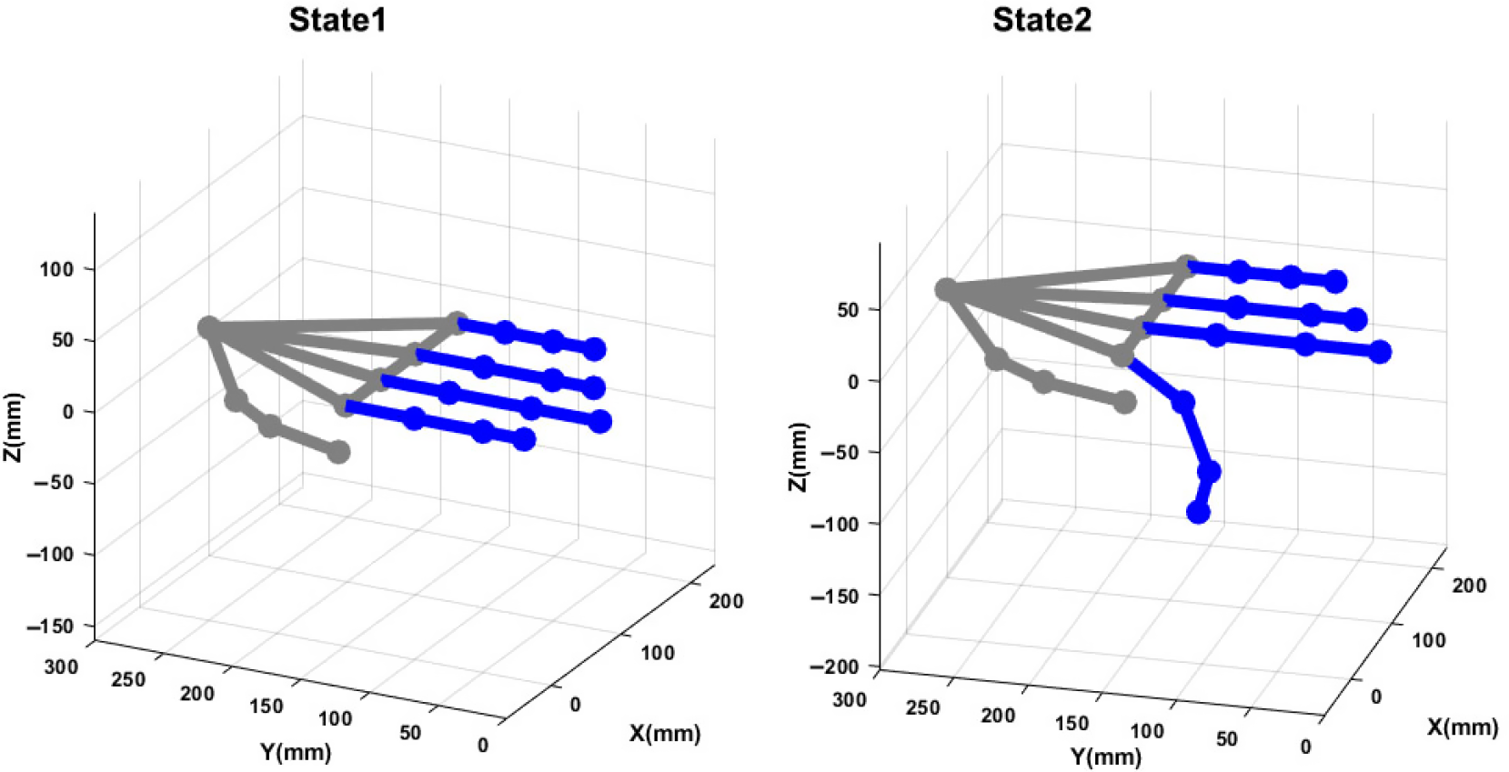
Figure 11. Hand posture reconstruction for flexed and flat states. The finger’s motion is captured with the designed sensing system.
6. Experimental modeling of soft actuator
The primary purpose of experimental modeling is to investigate kinematic compatibility, appropriate performance, and safe interaction of the designed actuator with the human hand’s structure by finger movement parameters such as ROM. Therefore, by considering the actuator as a black box system, empirical models are derived for both free motion and interaction with environment based on the experimental data obtained from the sensing system introduced in the previous sections.
To model, the polynomial model structures and artificial neural networks as standard data-driven techniques are employed, and both methods are endorsed by using external datasets to approximate their prediction accuracy. The experimental setup is shown in Fig. 12 is used to generate sufficient experimental data describing the actuator’s behavior under different operating conditions. This setup is designed according to the schematic diagram illustrated in Fig. 1.
6.1. Free actuator modeling
Regarding that bending with a constant curvature is an intrinsic specification in continuum soft robots, utilizing two IMUs is adequate to capture the final position of the free actuator after applying pressure. As shown in Fig. 13, one of the integrated IMUs is attached to the distal end, and the other one is to the proximal end as a reference.
Tree parameter identifications are considered to assess the actuator’s behavior relative to the applied pressure in the quasi-static state: time vector, angle change vector, and pressure change vector. An example of complementary motion of the bending is shown in Fig. 14. The test includes ramp responses in different amplitudes, each of which starts the initial state from its predecessor’s final state. Thanks to the unstable behavior of the actuator against a step input, ramp inputs are applied for identification purpose. Furthermore, since adding the initial orientation of the actuator to the model enhance the accuracy of prediction, this type of input can be considered an appropriate one [Reference Elgeneidy, Lohse and Jackson29]. It should be noted that the amplitude of applied pressure is determined based on the actuator’s minimum and maximum capacity.
Tree system identification methods as parametric model structures are applied to represent the system. These methods are the autoregressive with exogenous input (ARX) model, autoregressive moving average with exogenous input (ARMAX) model, and output-error (OE) model. In fact, the plant model will be extracted in these identification methods by analyzing the relation between input-output data. However, measured data is subject to measurement noise in real-world applications. Thus, to assess the effects of noise and simulate practical conditions, the identification process in the presence of noise is considered. In other words, white noise is created through a random signal with a standard normal distribution added to the system response signal.
To specify the dynamic order in the mentioned models, parameters such as initial delay time, final input, and output delay time, the order of polynomial in the transfer function model need to be specified. For this reason, several models with different orders are considered, and for evaluating the quality of the model, final prediction error (FPE) and best fit (FIT) measurement criteria, depicting the percentage of actual and simulated data matching, are assessed. The optimal values of the parameters are shown in Table IV. These parameters include model order of the observed state (
 $n_{a}$
), model order of the control signal (
$n_{a}$
), model order of the control signal (
 $n_{b}$
), model order of error (
$n_{b}$
), model order of error (
 $n_{c}$
), and the pure delay model (
$n_{c}$
), and the pure delay model (
 $n_{k}$
).
$n_{k}$
).
Table III. Verification result of repeatability experiment for flat and flexed states of the index finger.


Figure 12. Experimental setup including soft actuator along with the sensing system and pneumatic system used for generating the dataset.

Figure 13. Experimental setup utilized to generate the dataset for the free actuator based on the sensing system output.

Figure 14. Input and output signals for parameter estimation (a) pressure (b) deflection.
The values with the highest curve fitting, lowest FPE, and complexity are chosen among the evaluated parameters. In this line, the results of the parametric system identification method exhibit that a second-order model is an appropriate trade-off between the model’s accuracy and complexity. In essence, the lowest amount of FPE can be obtained through the ARX model, and in this model, FPE values decline up to
 $n=2$
and
$n=2$
and
 $m=2$
, and then it changes on a small scale. Hence, the model orders can be considered as
$m=2$
, and then it changes on a small scale. Hence, the model orders can be considered as
 $n=m=2$
. The output of the estimated and actual systems are compared in Fig. 15.
$n=m=2$
. The output of the estimated and actual systems are compared in Fig. 15.
The mathematical model of the actuator can be estimated according to the (10). The Nyquist stability criterion is employed to analyze the stability and frequency behavior of this transfer function. According to this theory, the number of unstable closed-loop poles must be equal to the number of unstable open-loop poles plus the number of encirclements of the Nyquist diagram around the critical point
 $(\!-\!1,0. j)$
. For this reason, since the Nyquist plot does not encircle the point
$(\!-\!1,0. j)$
. For this reason, since the Nyquist plot does not encircle the point
 $(\!-\!1,0. j)$
as shown in Fig. 16, while there exists an unstable open-loop pole, the overall system is unstable, necessitating the designing of controllers to recuperate the system stability.
$(\!-\!1,0. j)$
as shown in Fig. 16, while there exists an unstable open-loop pole, the overall system is unstable, necessitating the designing of controllers to recuperate the system stability.
 \begin{equation}G(s)=\frac{Y(s)}{U(s)}=\frac{107.8 s^{2}-107.8s}{0.2971 s^{2}+0.7024 s-1} \end{equation}
6.2. Modeling of the free actuator with artificial neural networks
As demonstrated in Section 6.1, the autoregression methods can predict the free actuator’s behavior with an accuracy of around 87%. To cope with uncertainty sources and achieve higher precision, the feed-forward ANN techniques, including multilayer perceptron (MLP) and radial basis function (RBF) neural networks, are employed for both the free and constraint states of the actuator. According to the actuator’s capacity and minimum barometric accuracy, the dataset is collected to train and validate designed networks. These network structures are found to decrease the RMSE while avoiding overfitting. The ANN models’ inputs are the values of the pressure sensor, and the target output is the angular displacement of the end section of the actuator relative to the reference sensor.
Table IV. Comparison of the regression statistics for the three derived models.


Figure 15. Comparison of the estimated polynomial models (ARX, ARMAX, OE) with the actual output.
Several MLP networks with one and two layers and 1–30 neurons are trained and validated for the hidden layer to determine the best structure. Training is conducted using the Bayesian regularization algorithm, which has better performance in comparison with Levenberg Marquardt to reveal complex relationships [Reference Kayri30]. However, the train of the network is time-consuming in this algorithm.

Figure 16. The stability analysis of the estimated ARX model of free actuator with Nyquist diagram.
The results demonstrate that the best MLP configuration contains one input layer and one input variable, two hidden layers with 15 and 12 neurons in each hidden layer, and one output layer with one output variable (Table V). In essence, this model can predict the actuator’s behavior with an RMSE of 0.711, a standard deviation of 0.963.
In the RBF neural network structure, as a single-layer neural network, the output is generated by mapping distances between the center vectors and input vectors to outputs through a nonlinear kernel or radial function [Reference Abiodun, Jantan, Omolara, Dada, Mohamed and Arshad32].
In this study, neuron numbers as the RBF centers in the hidden layer are selected from a series of trial runs of the networks to reach minimum error. Results depict that an RBF network with 48 neurons in the hidden layer can achieve an RMSE of about 0.661 and standard deviation of 0.997 (Table VI).
It is worth mentioning that input–output data for networks training is the same as that used to extract the regression models. Comparison of ANNs with the best performing regression model (ARX) reveals that ANN models, especially the RBF one, obtain a higher best fit and lowest FPE (Table VII). Regarding this, ANN-MLP and ANN-RBF have a better performance than regression models for predicting angels. This is because trained networks can estimate the nonlinear response of the soft actuator with higher precision, for which the linear regression model cannot account. Thus, the better performance of the ANN models can be justified by the capability of capturing highly nonlinear relationships in data, even when the precise nature of such relationships is obscure [Reference Kumar, Aggarwal and Sharma31].
In this step, the bending calculated by the sensing system and the bending predicted by the ANN and autoregressive models is compared. The results demonstrate an accurate fit between the inputs and the target output of the RBF model in comparison with the MLP and regression models (Fig. 17).
6.3. Modeling of the constrained actuator with artificial neural networks
Since the angular motion and stiffness of the finger’s joints affect the actuator’s performance, the estimated models for the free actuator cannot be generalized to the actuator constrained to the finger. Thus, a high-precision model is required when the actuator is in interaction with the finger. The ROM at the three points of the actuator (Fig. 18), which are tied to the three index finger joints, and pressure changes are determined as target outputs and input, respectively. The structure shown in Fig. 19 is utilized to generate a dataset for the network training.
Table V. MLP-ANN error statistics at different numbers of hidden layers and neurons.

Table VI. RBF-ANN error statistics at different numbers of hidden layers and neurons.

Table VII. Comparing prediction accuracy statistics of the trained ANNs, and ARX regression model.


Figure 17. Comparing the prediction accuracy of trained ANNs, ARX regression model, and target angle attained through the sensing system.

Figure 18. Schematic demonstration of the flexed soft actuator and the definition of the relative angle and at MCP, PIP, and DIP joints.
As in Section 6.2, after investigating statistical parameters values for MLP and RBF networks, an MLP network with one input layer and three input variables, two hidden layers with 20 and 25 neurons in each hidden layer, and one output layer with three output variables can predict the actuator’s actuator behavior with an RMSE of 0.981. Besides, an RBF network with 56 neurons in the hidden layer can reach an RMSE of 0.964.
The performance and accuracy of the implemented ANN are evaluated with an external dataset. As presented in Table VIII, the ANN model networks can predict the value of the relative angles between the actuator and joints as defined in Fig. 18 with the error values less than 1
 $^\circ$
for MCP, PIP, and DIP. Also, an appropriate fit between the inputs and the target output is shown in Fig. 20. As shown, the bending amplitude of the actuator is significantly reduced due to the restriction to the finger.
$^\circ$
for MCP, PIP, and DIP. Also, an appropriate fit between the inputs and the target output is shown in Fig. 20. As shown, the bending amplitude of the actuator is significantly reduced due to the restriction to the finger.

Figure 19. Experimental setup for motion analysis of the soft actuator interacting with the index finger. This setup includes the soft actuator accompanying a 3D-printed finger prosthetic and the sensing system.
Table VIII. Error statistics of the trained ANNs for the index finger’s joints.


Figure 20. Comparing prediction output of trained ANN and measured angular motion of the actuator’s sections at MCP, PIP, and DIP joints while interacting with an index finger during flexion and extension.
7. Conclusion
In this study, a pneumatically actuated soft robotic equipped with an IMU-based sensing system is developed for index finger rehabilitation. The KF is employed as an attitude fusion algorithm to eliminate the drift effect on gyroscope data and mechanical and electrical noise of the raw acceleration data. Regarding the importance of kinematic analysis, static and dynamic angle validations are also conducted to assess the accuracy and reliability of the sensor fusion algorithm. The obtained precision in static and dynamic states demonstrates that the sensing system is optimal and reliable in rehabilitation applications (<3
 $^\circ$
). Compared with the other proposed IMU-based sensing systems, this cost-effective system can significantly decline the drift effect without using the magnetometer data, which is highly susceptible to external magnetic fields.
$^\circ$
). Compared with the other proposed IMU-based sensing systems, this cost-effective system can significantly decline the drift effect without using the magnetometer data, which is highly susceptible to external magnetic fields.
Furthermore, an alternative approach is developed to predict the angular displacement of a standard soft pneumatic actuator. This approach is based on data-driven modeling techniques, relying on generated datasets of a sensing system feedback without the need for deriving complicated material and physical models. Basically, parametric system identification methods, artificial multilayer perceptron, and radial basis function neural network algorithms are employed to predict the change of bending angle during the actuation. In order to validate the derived experimental models, a new dataset generated at untrained operating conditions is used. The comparison of the results shows that both techniques successfully predict the bending response of the soft actuator. However, neural networks, notably RBF ones, provide more accurate predictions because of capturing highly non-linear relationships in the data.
The main contribution of this study is in deriving reliable empirical models through data-driven modeling approaches to enable individuals to have effective control over soft actuators in the rehabilitation field. Indeed, the feedback from inexpensive commercially IMU sensors eliminates the need to attain prior knowledge about a soft actuator’s material characteristics and geometry. Another contribution is designing a home-based rehabilitation device using a soft actuator that can continuously record the joint’s motion. Although several soft robotic exoskeletons have been developed for hand rehabilitation, limited numbers have focused on using a precise and constant sensing mechanism. Consequently, this rehabilitation robot is an appropriate tool to capture and model an index finger’s anatomical motion interacting with a soft pneumatic actuator.
Overall, our proposed system can assist the treatment of hand dysfunction in patients with motor disorders in clinical settings and activities of daily living owing to its soft, lightweight, and user-friendliness design [Reference Chu and Patterson33]. In other words, it allows quantitative assessment of the active ROM and functionality of the hand along with providing safe human-robot interaction. Accordingly, it can widely be employed as an assistive robot to improve post-stroke motor dysfunction and spasticity [Reference Ansari, Manti, Falotico, Mollard, Cianchetti and Laschi34, Reference Heung, Tang, Shi, Tong and Li35].
In future research, the developed models will be applied to design a control algorithm using real-time feedback from the sensing system. Moreover, this prototype will be extended to capture the motion of other fingers to evaluate the system’s effectiveness on stroke patients in the clinical setting.


