


1. Introduction
When devising poverty reduction strategies in the face of climate change, the role of environmental risks in the livelihoods of poor people needs to be understood. First, people struggling with multiple environmental risks generally have a lower ability to cope with other shocks and are thus more vulnerable to climate change impacts. Second, climate change will directly exacerbate weather-related environmental risks, such as rainfall and temperature variability and extremes and thereby increase this baseline vulnerability. Accordingly, poor people already exposed to high environmental risks could be most affected by climate change.
The interlinkages between poverty and environmental risks have been reviewed in earlier papers covering the extensive literature on this topic (Reardon and Vosti, Reference Reardon and Vosti1995; Duraiappah, Reference Duraiappah1998; Scherr, Reference Scherr2000; Gray and Moseley, Reference Gray and Moseley2005; Barbier, Reference Barbier2010, Reference Barbier2012; Barrett et al., Reference Barrett, Travis and Dasgupta2011). Environmental risks are unevenly distributed across space – depending on geographic and climatic conditions, as well as socioeconomic factors that condition them. Poor people often live in remote and fragile areas, with high levels of environmental risks, where they overly depend on the use of ecosystems and natural resources, which can increase ecosystem fragility and environmental risks. This downward spiral could result in spatial poverty traps, where pockets of fragility, risks, marginalization and poverty persist (Carter et al., Reference Carter2007; Barbier, Reference Barbier2010; Barrett et al., Reference Barrett, Travis and Dasgupta2011). These poverty traps could be further exacerbated by climate change.
To guide policies to break out of these traps, there is a need for more in-depth, spatial analyses which try to disentangle the relationship between environmental risks and poverty (Barbier, Reference Barbier2012). While there is ample empirical work showing a positive relationship between environmental risks and poverty at the global and regional levels (e.g., Chomitz et al., Reference Chomitz2007; Barbier, Reference Barbier2010, Reference Barbier2015; Sloan and Sayer, Reference Sloan and Sayer2015), the national and sub-national levels (e.g., Dasgupta et al., Reference Dasgupta2005; Bandyopadhyay et al., Reference Bandyopadhyay, Shyamsundar and Baccini2011; Winsemius et al., Reference Winsemius2015) or in specific locations (Khan and Khan, Reference Khan and Khan2009; Watmough et al., Reference Watmough2016), all this work together points to a complex picture, where the relationship depends on the specific types of risks and locations of interest, as well as the channels through which they interact. New, high-resolution spatial data, for example from remote sensing, allows us to analyze the distribution of environmental risks and poverty across space in order to better understand the multifaceted nature of this relationship.
Vietnam provides an interesting case study for such an analysis. Despite a reduction of extreme poverty from around 60 per cent in 1990 to 13.5 per cent as of 2014 (World Bank Group, Reference World2016),Footnote 1 pockets of poverty still exist today: 91 per cent of people in extreme poverty live in rural areas and belong to marginal groups, such as ethnic minorities, who have a poverty rate of about 58 per cent (Kozel, Reference Kozel2014). At the same time Vietnam is facing various environmental challenges. Land is increasingly degraded by human-induced factors (Vu et al., Reference Vu2014a, b). Although total tree cover has increased, certain areas suffer from high rates of forest loss and degradation (Pham et al., Reference Pham2012). Air pollution is an increasing concern (Luong et al., Reference Luong2017). And weather variability and extreme events, such as floods and droughts, severely affect livelihoods (Thomas et al., Reference Thomas2010; Bui et al., Reference Bui2014; Arouri et al., Reference Arouri, Nguyen and Youssef2015; Narloch, Reference Narloch2016). An earlier spatial analysis at the provincial level in Vietnam, however, finds that the relationship between poverty and environmental risks is hard to generalize (Dasgupta et al., Reference Dasgupta2005).
This paper revisits this relationship, taking advantage of more recent and higher-resolution data to examine four research questions: (RQ1) At the district level, is the incidence of poverty higher in high risk areas? (RQ2) At the household level, do poor households face higher environmental risks? (RQ3) Does the relationship between household-level consumption and environmental risks vary between rural and urban areas? (RQ4) Do environmental risks relate to consumption differences between households and consumption changes over time? On their own, many of these questions have been addressed in the existing literature, but they have hardly been brought together to draw a comprehensive picture of the relationship between poverty and multiple environmental risks within a single country context using high-resolution data. We contribute to existing work by assessing how the relationship between poverty and multiple dimensions of environmental risk varies as a function of the channels through which poverty and risk interact, using a set of consistent data and methods while holding constant national context.
In this paper a number of recently-developed high-resolution datasets are used to separately assess eight environmental risks: (i) outdoor air pollution as a proxy for health risks through respiratory diseases (from Brauer et al., Reference Brauer2015); (ii) tree cover loss as a proxy for the loss of forest resources and ecosystem functions (from Hansen et al., Reference Hansen2013); (iii) land degradation as a proxy for productivity decline and agricultural production risks (from Vu et al., Reference Vu, Le and Vlek2014b); (iv) slope as a proxy for areas vulnerable to erosion and landslides (from World Soil Database); (v-vi) long-term rainfall and temperature variability as a proxy for the variation of weather conditions (from the Climate Research Unit (CRU)); (vii) flood hazards as a proxy for rainfall- and coastal-related extreme events (from Bangalore et al., Reference Bangalore, Smith and Veldkamp2016); and (viii) drought hazards as a proxy for drought events (from Winsemius et al., Reference Winsemius2015).
These data are combined with national maps showing the incidence of poverty at the district level in 2010 (Lanjouw et al., Reference Lanjouw, Marra and Nguyen2013). In addition, this study computes environmental risks at the commune levelFootnote 2 to relate it to household information based on the latest Vietnam Household Living Standard Surveys (VHLSS) for 2010, 2012, and 2014 to examine whether environmental risks vary between households. Benefiting from the panel structure of these surveys, we also assess how environmental risks are related to consumption changes over time.
The remainder of this paper is structured as follows. Section 2 starts by deriving four research questions regarding the environmental risk and poverty linkages from existing literature. Section 3 describes the data used for the analysis of these research questions. The following four sections present the results. Section 4 shows the district-level overlay of environmental risks and poverty in 2010 (RQ1). Section 5 compares environmental risks at the commune level across household groups (RQ2). Building on these analyses, section 6 investigates differences in the relationship between household consumption levels and environmental risks between rural and urban areas (RQ3). Section 7 deepens these analyses by presenting results from various regression models explaining consumption differences between households and changes over time by environmental risks at the commune level (RQ4). Section 8 concludes.
2. Conceptual framework
What do we know about the association between environmental risks and poverty? Intuition suggests that the two are positively associated: the higher the level of environmental risk, the higher the incidence of poverty (conversely, the lower the level of consumption). While empirical work lends some support to this claim, the relationship is multifaceted. In this section, we examine dimensions over which poverty and environmental risks might vary: (1) across risk, space, time, and scale, (2) between rural and urban areas, and (3) depending on the channels that determine the relationship. While the framework presented below does not fully address all the different dimensions and causes that underpin this complex relationship and is not supposed to integrate the full set of frameworks existing in this field, it does serve to motivate the empirical approach taken in this paper, which is to examine the multifaceted relationship across many risks in the single context of Vietnam.
2.1 Differences across risk, space, time, and scale
The literature associated with the environmental Kuznets curve (Panayotou, Reference Panayotou1997) argues that the relationship between environmental risks and incomes might be inversely U-shaped, with environmental degradation increasing with income levels up until a threshold is reached, after which degradation rates decrease. While consistent and rigorous evidence for this hypothesis has not been confirmed across a wide range of studies (for a review, see Stern, Reference Stern2004), the framework highlights the fact that the relationship between environmental risks and poverty is not monotonic or straightforward.
Nevertheless, a range of studies in the literature point to a positive relationship between environmental risks and poverty. At the global level, various studies show that environmental risks are higher in poorer countries (Barbier, Reference Barbier2010, Reference Barbier2015; Barrios et al., Reference Barrios, Bertinelli and Strobl2010; Sloan and Sayer, Reference Sloan and Sayer2015). Studies at the sub-national level show that in some high-risk provinces and districts, the incidence of poverty is higher (Dasgupta et al., Reference Dasgupta2005; Winsemius et al., Reference Winsemius2015; Watmough et al., Reference Watmough2016). Similarly, at the household level, poorer households are found to have a higher exposure to some environmental risks than wealthier households (Ranger et al., Reference Ranger2011; Akter and Mallick, Reference Akter and Mallick2013; Wodon et al., Reference Wodon, Liverani and Joseph2014). Yet overall the findings are mixed and very context dependent.
First, the relationship depends on the specific risk being considered. For example, Hallegatte et al. (Reference Hallegatte2016) find that within countries, poorer areas are also more exposed to higher temperatures and drought, but not to floods. In terms of air pollution, poor people tend to be more exposed to both ambient (outdoor) but also indoor air pollution. For outdoor air pollution, studies focused mostly in the developed world find that polluting industries (including coal plants) often locate in lower-income neighborhoods (Braubach and Fairburn, Reference Braubach and Fairburn2010). In terms of indoor air pollution, poorer households in developing countries remain highly reliant on firewood or biomass for cooking, with women and children living in severe poverty having the highest exposure levels (Gordon et al., Reference Gordon2014). One recent study that has looked at different environmental risks in Lao PDR finds strong connections with poverty for indoor air pollution and water quality, weak connections for deforestation and soil erosion and no connection for outdoor air pollution (Pasanen et al., Reference Pasanen2017).
For some environmental risks, even a negative relationship could exist, resulting from economic development that has increased welfare levels but degraded ecosystems, such as agricultural intensification or land expansion into natural areas. For example, rural households in sub-Saharan Africa, many of whom are poor, often rely on charcoal production to support growing demand in urban areas. While this contributes to poverty reduction through income-generation opportunities, it can also undermine soil and ecosystem stability and thereby agricultural production (Zulu and Richardson, Reference Zulu and Richardson2013). Generally, deforestation can deprive rural households of natural resources they depend on, while at the same time providing new income sources (Chomitz et al., Reference Chomitz2007; Laurance et al., Reference Laurance, Sayer and Cassman2014). Where these contrasting effects coexist, it is possible that no significant relationship between degradation and poverty can be found.
More generally, within a country, the relationship between environmental risks and poverty is likely to change over time. For instance, Ebenstein et al. (Reference Ebenstein2015) observe that over the period of 1991–2002, China increased incomes and reduced poverty, as well as increasing air pollution. While high levels of air pollution increased mortality rates, economic growth and poverty reduction have also been associated with other health improvements that likely outweighed air pollution impacts. Also, where ecosystems have already been degraded substantially in the past, further degradation will be limited. Such change over time may explain why areas with low soil erosion rates tend to be poorer (Naipal et al., Reference Naipal2015).
Generally, poverty and environmental risks are unevenly distributed across space so that the relationship also depends on the places considered. The spatial distribution of environmental risks and poverty varies greatly between countries, being shaped by a combination of agro-climatic and socio-economic conditions (Tucker et al., Reference Tucker2015). Even in geographically similar countries, different patterns can be observed, as shown by Dasgupta et al. (Reference Dasgupta2005): while in Lao PDR there is a spatial correlation between poverty and all environmental risks, in Cambodia, poverty is only positively related to household-level risk factors, such as indoor air pollution and lack of access to adequate water and sanitation. For Vietnam, the authors only find a positive relationship with fragile soils and indoor air pollution.
Moreover, the scale of the analysis matters too. For example, Winsemius et al. (Reference Winsemius2015) find mixed evidence for a higher exposure of poor people to climate-related risks, such as floods, when looking at poverty and risk levels at the district level. This finding could emerge because even within a district, poverty and risks may be very unevenly distributed, so more granular data at the local level from household surveys or case studies is needed. Indeed, looking at the same risk within a city – Mumbai, India – Ranger et al. (Reference Ranger2011) find that poorer households in Mumbai are almost twice as exposed to floods.
However, analyses at higher resolution (e.g., household level) do not always show a positive association between environmental risks and poverty. Various studies show that there is no considerable difference between poor and wealthier households in their exposure to natural disaster risks (del Ninno, Reference del Ninno2001; Carter et al., Reference Carter2007; Opondo, Reference Opondo2013). These findings may be explained by the scale of the risk (in some cases, everyone is exposed as in the case of drought), but highlight that the relationship between poverty and exposure to environmental risks is context specific and depends on the type of hazard, local geography, institutions and other mechanisms (Hallegatte et al., Reference Hallegatte2016).
Thus overall the relationship between environmental risks and poverty remains an empirical question that depends on the specific risk types and locations of interest and the scale considered. Accordingly, it needs to be tested whether patterns at the provincial or district level hold at the household level. From this we derive our first and second research questions, (RQ1) and (RQ2), regarding the relationship between risks and poverty at different scales: (RQ1) Is the incidence of poverty (P) at the district level higher in high risk areas than low risk areas? And (RQ2), at the household level is the level of environmental risks (R) higher for poor than for non-poor households?
 $$\eqalign{\hbox{District}-\hbox{level}: P_{{\rm High \ Risk \ Areas}} > P_{{\rm Low \ Risk \ Areas}}}$$
 $$\eqalign{\hbox{Household}-\hbox{level}: R_{{{\rm Poor}}} > R_{{{\rm Non}}-{{\rm Poor}}}}$$
2.2 Differences between rural and urban areas
While various studies address the relationship between environmental risks and poverty in rural or urban areas, so far not many studies have examined differences between rural and urban spaces within the same country. Yet the extent of poverty, as well as the spatial distribution of poor people in the countryside, can differ substantially from cities, so the relationship between environmental risks and poverty could also vary.
First of all, rural and urban areas differ in wealth levels and thus the incidence of poverty. Rural areas have generally lower consumption levels and poverty continues to be mostly a rural problem. In 2012, 78 per cent of the global population in extreme poverty was living in rural areas (Olinto et al., Reference Olinto2013). At the same time, more and more destitute people are moving into cities in search of new opportunities, so inequalities in urban areas may be increasing (Fox, Reference Fox2014). In many countries, rural populations are concentrated in fragile areas with higher levels of environmental risks, including land degradation (Barbier, Reference Barbier2010) and terrain ruggedness (Nunn and Puga, Reference Nunn and Puga2012). While some hotspots where high risks and poverty coincide can be found, environmental risks could also be higher in wealthier areas (Pasanen et al., Reference Pasanen2017). Many case studies show how marginal people in rural areas face environmental risks: for example, precipitation variability in the Peruvian Andes (Sietz et al., Reference Sietz, Choque and Lüdeke2012), floods in Senegal (Tschakert, Reference Tschakert2007), drought in the Sahel (Sissoko et al., Reference Sissoko, van Keulen, Verhagen, Tekken and Battaglini2011) and Northwest China (Li et al., Reference Li2013), and cyclone-related saltwater intrusion in coastal Bangladesh (Rabbani et al., Reference Rabbani, Rahman and Mainuddin2013). However, within rural areas, it is unclear whether poor people are more exposed than non-poor people. For instance, areas of higher forest cover loss might have lower poverty rates due to the income-generation opportunities associated with agricultural expansion or forest products (Chomitz et al., Reference Chomitz2007; Laurance et al., Reference Laurance, Sayer and Cassman2014).
In urban areas, the differences in exposure between poor and urban households could be more pronounced. Land scarcity is more pressing in urban areas, such that poor people (especially migrants) tend to locate in cheaper parts of the city and end up in slums (Fay, Reference Fay2005). Often, these slum areas are characterized by higher environmental risks which are reflected in the price of land (Fay, Reference Fay2005): for instance, Lall and Deichmann (Reference Lall and Deichmann2012) observe that the parts of Bogota which experience the highest earthquake risk are also the cheapest, and are where most of the poor locate. Accordingly, Winsemius et al. (Reference Winsemius2015) find a positive association between flood risk and poverty within urban areas, but do not find the same association at the national level, suggesting land prices to play a key role in determining exposure to environmental risks in cities.
More generally, differences across poverty levels in rural-urban settings may reflect the differing role of natural resources: whether they are primarily an input to production or to environmental quality (Panayotou, Reference Panayotou, Haen, Wilk and Harnish2016). For instance, forests may be used as a production input in rural areas so that they become increasingly degraded with higher wealth levels. In urban areas they may be seen as an environmental quality amenity and hence become more protected with higher wealth levels. While these differing roles of natural resources, such as forests, can help explain findings in previous studies, such a framework cannot be used for all the environmental risks which we explore in this paper.
In this context, it is of interest to understand whether poor people live in riskier places in rural and urban areas alike. Hence our third research question (RQ3) focuses on the difference in the relationship between environmental risks and poverty within rural and urban areas: Is the correlation between environmental risks (R) and poverty (P) positive (or negative for consumption levels) in rural as well as urban areas?
 $$\hbox{corr}\ (R_{{{\rm Rural}}}, P_{{{\rm Rural}}} )>0 \hbox{and corr } (R_{{{\rm Urban}}}, P_{{{\rm Urban}}} ) > 0$$
2.3 Different causes
So far, we have discussed whether there is a positive relationship between environmental risks and poverty, but not the reasons behind this relationship. There can be multiple, interlinked channels that determine this relationship.
First, poor people and fragile areas could have shared vulnerabilities (Barrett et al., Reference Barrett, Travis and Dasgupta2011). For example, adverse hydroclimatic conditions could increase flood and drought hazards as well as ecosystem fragility, while also making livelihood activities, such as agriculture, more difficult, thereby resulting in lower incomes and consumption. For instance, dry climate zones in sub-Saharan Africa are vulnerable to precipitation deficits due to poor soils with low moisture storage capacity and host rural people who remain poor as they are reliant on low-return and high-risk agricultural activities (Zimmerman and Carter, Reference Zimmerman and Carter2003; Barrios et al., Reference Barrios, Bertinelli and Strobl2010).
Second, poverty and environmental risks can be determined by common factors, such as institutional and market failures (Duraiappah, Reference Duraiappah1998; Barbier, Reference Barbier2010; Barrett et al., Reference Barrett, Travis and Dasgupta2011). For example, where property rights for land are missing, it is more likely that environmental resources, such as timber and fish, are overexploited (Baggio and Papyrakis, Reference Baggio and Papyrakis2010). At the same time, powerful actors can oust poor people without land title from land, leaving them without their main asset for wealth accumulation (Grainger and Costello, Reference Grainger and Costello2014). These institutional failures can also be related to market failures, where environmental services, such as water and soil regulation, are not factored into market prices. While this lack of a price signal can lead to an underprovision of these services and hence higher risks, poor people managing ecosystems sustainably are not paid for this service provision.
Third, poverty could increase environmental risks (Duraiappah, Reference Duraiappah1998; Barbier, Reference Barbier2010; Barrett et al., Reference Barrett, Travis and Dasgupta2011). Many poor people – especially those in rural areas – depend on ecosystems for their livelihoods. For example, a systematic analysis of a 28-country data set shows that in (sub-) tropical smallholder systems, the poorest households derive more than half of their income from ecosystems and that this share is higher than for the wealthiest households (Angelsen et al., Reference Angelsen2014; Noack et al., Reference Noack2015). These incomes often play a role in consumption smoothing between seasons or as a coping mechanism when other incomes fail (Locatelli et al., Reference Locatelli, Pramova and Russell2012). Although environmental extraction may not be a primary coping strategy (Wunder et al., Reference Wunder2014), ecosystem-based incomes are a substitute for other incomes and can stabilize total incomes when weather anomalies hit (Noack et al., Reference Noack2015). In addition, where poor people lack other opportunities, they may disproportionally resort to overexploiting natural resources (e.g., timber, fish or grassland) for short-term survival – a strategy that can cause poverty traps (Barbier, Reference Barbier2010; Barrett et al., Reference Barrett, Travis and Dasgupta2011).
Fourth, environmental risks could increase poverty (Duraiappah, Reference Duraiappah1998; Barbier, Reference Barbier2010; Barrett et al., Reference Barrett, Travis and Dasgupta2011). Where people depend on ecosystems as a safety net or for their base income, any environmental risks that undermine these functions will reduce their incomes and consumption. In (sub-)tropical smallholder systems, an additional 13 per cent of households would be in poverty without ecosystem-based incomes (Noack et al., Reference Noack2015). Moreover, the occurrence of natural disasters can have a direct impact on welfare, pushing people back into poverty or making it harder for poor people to escape poverty: for instance, in Bolivia, poverty rates increased by 12 per cent in Trinidad city after the 2006 floods (Perez-De-Rada and Paz, Reference Perez-De-Rada and Paz2008; Hallegatte et al., Reference Hallegatte2017). Households that lack ex-post coping mechanisms often seek to mitigate risks ex-ante, for example through income diversification, thereby lowering average consumption and income (Bandyopadhyay and Skoufias, Reference Bandyopadhyay and Skoufias2015). The extent to which the exposure to risks, without the materialization of an immediate direct impact on consumption and incomes, such as forest or land degradation, can affect poverty has been less explored, and links are difficult to disentangle due to feedback loops and synergistic effects (Gerber et al., Reference Gerber, Nkonya, von Braun, von Braun and Gatzweiler2014). Where the exposure to such risks has a negative effect on consumption and incomes, it is important to not only focus on risk response, but to derive strategies for risk reduction.
Hence it is important to understand whether risk exposure increases poverty or reduces consumption and income growth. While the other channels of the environment-poverty nexus are not less important, our fourth research question (RQ4) focuses on this channelFootnote 3: do environmental risks (R) increase poverty (P) (or reduce consumption)?
 $$P = f(R) \hbox{or } R\to P$$
3. Data
This study combines socioeconomic data from the Living Standard Measurement Surveys (VHLSS) in 2010, 2012, and 2014 measuring household-level consumption, and recent geo-spatial data measuring environmental risks at high resolution. These two data types are merged at the district and commune levels.
3.1 Socioeconomic data
The VHLSS 2010, 2012, and 2014 are nationally and regionally representative and contain detailed information on individuals, households and communes.Footnote 4 In total 9,400 households nationwide are included in each round. A particularity of the VHLSS data is that half of these households were interviewed in two or three of these survey years. These households form a short-term ‘Panel’ dataset to explain consumption changes over time. Other households were only observed in one of the three years. Using these cross-section data, treating all observations as independent observations provides a ‘Pooled’ dataset to explain consumption differences between households. In rural areas, 6,600–6,750 households from about 2,200 communes in each year are included (‘Pooled’ cross section). Of these, 1,400 are observed in all three rounds, 1,600 are observed in 2010 and 2012, and 1,400 are observed in 2012 and 2014 (‘Panel’ dataset). In urban areas, the dataset covers 2,650–2,780 households in each year from 900 communes (‘Pooled’). Of these, 500 are in all three rounds, 575 in 2010 and 2012, and 640 in 2012 and 2014 (‘Panel’).
The VHLSS data provide detailed information to estimate consumption values based on expenditure data. Section 4 uses district-level poverty maps. The ratio and number of people below the national poverty lineFootnote 5 in each district is estimated using the consumption values from the VHLSS 2010 combined with the 15 per cent sample of the 2009 Population and Housing Census as calculated by Lanjouw et al. (Reference Lanjouw, Marra and Nguyen2013). Sections 5 and 6 use consumption values from the VHLSS 2014 and section 7 adds the data from the 2010 and 2012 surveys. All consumption values are calculated in line with the methodology for determining the national poverty line.Footnote 6
This data from Lanjouw et al. (Reference Lanjouw, Marra and Nguyen2013) is used to examine RQ1. Through our own calculations, we use the 2014 VHLSS to examine RQ2 and RQ3, while we use all three rounds (2010, 2012, and 2014) to examine RQ4.
The household and commune surveys in the VHLSS 2010, 2012, and 2014 also include a wide array of data on socioeconomic conditions. Data at the individual level include demographics, education, employment, health and migration. At the household level, data comprise information on durables, assets, production, income and participation in government programs. The commune surveys collect information about the commune characteristics including access to land, infrastructure and services. Based on these data, a number of socioeconomic controls are constructed for the analyses based on household and commune surveys (the summary statistics can be found in the online appendix, table A.1).
3.2 Environmental risk data
Based on geo-spatial datasets, variables are constructed to measure environmental risk at district and commune levels representing eight environmental risks. These variables are based on historical risk profiles measuring the area's exposure to fragile and severe conditions and not the actual environmental conditions at the time of the VHLSS surveys. The following variables are calculated to measure the area-weighted average of each environmental risk at the district and commune level (the summary statistics can be found in table A.1)Footnote 7:
(1) Air pollution is measured by the area-weighted mean of concentration (measured as micrograms per cubic meter) of particulate matter with a diameter of 2.5 micrometers or less (PM2.5) taking the 10 year-average value for 2000–2010. The data is based on satellite imagery using the total column aerosol optical depth from the Moderate Resolution Imaging Spectroradiometer (MODIS) and Multiangle Imaging Spectroradiometer satellite instruments, which is combined with chemical transport model simulations, and ground measurements from 79 countries to produce a global spatial dataset with 0.1 × 0.1 resolution (Brauer et al., Reference Brauer2015). PM2.5 includes dust, dirt, soot, smoke and liquid droplets, which can lodge deeply into the lungs due to their small size. PM2.5 air pollution has been identified as a leading risk factor in diseases globally (Forouzanfar et al., Reference Forouzanfar2015) as well as in Vietnam (Luong et al., Reference Luong2017).
(2) Tree cover loss is calculated as the share of the area under tree cover in 2000 that suffered from a tree cover loss between 2000 and 2010. Tree cover is defined as canopy closure for all vegetation taller than 5 m in height and is calculated from imagery from the Landsat 4, 5, 7, and 8 satellite data used to produce a global forest cover change map (Hansen et al., Reference Hansen2013). Tree cover loss can be associated with a habitat disturbance and ecosystem service disruptions, which can make human landscapes more fragile to other impacts (Sodhi et al., Reference Sodhi2010). It can also undermine the livelihoods of poor people highly dependent on forest timber and other resources (Angelsen et al., Reference Angelsen2014).
(3) Land degradation is measured by the share of land area that experienced a significant biomass decline. This loss is calculated based on the inter-annual mean trend of Normalized Difference Vegetation Index based on data from the Advanced Very High Resolution Radiometer (AVHRR) of the National Oceanic and Atmospheric Administration (NOAA) satellite between 1982 and 2006, which is corrected for climate effects to only measure human-induced degradation (Vu et al., Reference Vu, Le and Vlek2014b). Soil ferti lity, agricultural productivity and ultimately food security of smallholder farmers can be largely compromised on degraded lands (Von Braun et al., Reference Von Braun2013).
(4) Slope is measured by the area-weighted average of slope categories. This variable is calculated based on data from the Harmonized World Soil Database version 1.2 with eight slope classes: 1 for least steep (elevation of 0–0.5 per cent) and 8 for most steep slope (elevation greater than 45 per cent).Footnote 8 Steep slopes are much more prone to surface water runoff and soil erosion – particularly in areas affected by heavy rainfalls and tree cover loss (Sidle et al., Reference Sidle2006; Vezina et al., Reference Vezina, Bonn and Van2006). At the same time, tropical cyclones can cause fatal landslides, which already result in significant loss of life in mountainous areas of South and East Asia (Petley, Reference Petley2010; Reference Petley2012).
(5) Rainfall variability is defined as the 1981–2010 standard deviation of monthly rainfall levels measured in millimeters (mm). The variable is constructed from the global CRU TS3.21 dataset from the University of East Anglia, containing a long-term time series of monthly rainfall levels at 0.5 × 0.5 grid resolution, which was produced using statistical interpolation based on data from 4,000 weather stations (Harris et al., Reference Harris2014). Higher historic rainfall variability indicates higher inter-annual and intra-annual variation of precipitation and a higher incidence of extremely wet and dry conditions. In Vietnam, excessive rainfall can have negative income effects for poor households, while wealthier households are more negatively affected by the lack of rainfall (Narloch, Reference Narloch2016).
(6) Temperature variability is measured by the standard deviation of mean annual temperatures across the time period 1981–2010 in degrees Celsius (C). The underlying data also comes from the global CRU TS3.21 dataset including a long-term time series of monthly mean temperature values at 0.5 × 0.5 grid resolution. Temperature variability indicates varying temperature conditions between seasons and years and a higher incidence of heat waves and cold spells. In Vietnam, hot conditions generally have an income-reducing effect for rural households (Narloch, Reference Narloch2016).
(7) Flood hazards are represented by the share of area at risk of a flood event (inundation depth >0) with a 25-year return period under historical conditions.Footnote 9 The measures are based on the inundation depth, estimated by state-of-the art flood models at a grid cell level of 3 arc-seconds combining coastal surge hazard layers, along with pluvial and fluvial layers (Bangalore et al., Reference Bangalore, Smith and Veldkamp2016). In Vietnam, flood events have been shown to significantly reduce welfare and increase poverty (Thomas et al., Reference Thomas2010; Bui et al., Reference Bui2014; Arouri et al., Reference Arouri, Nguyen and Youssef2015).
(8) Drought hazards are measured by the area-weighted intensity of drought conditions. This intensity is a measure of hydrological droughts and is expressed by the number of months of long-term mean discharge which would be needed to overcome the maximum accumulated deficit volume during dry months (Winsemius et al., Reference Winsemius2015). Drought events in Vietnam are associated with agricultural production losses, negative welfare impacts and poverty (Thomas et al., Reference Thomas2010; Bui et al., Reference Bui2014; Arouri et al., Reference Arouri, Nguyen and Youssef2015).
3.3 Data limitations
There are several limitations in using these datasets for the purpose of this study. Nevertheless, these data allow us to provide some interesting insights into our research questions.
First, while the data is representative of socio-economic conditions of the entire country, its eight regions and rural and urban areas, it is not representative of the different environmental risk profiles across communes. Building the living standard measurement survey (LSMS) methodology, the sampling strategy follows a three-stage stratified cluster design, whereby about one-third of all communes are selected and divided into three areas from which one area is chosen and three households are interviewed from these areas (ISM and SINFONICA, 2015). Due to this strategy, the entire variety of communes is not represented and communes in very remote areas and with extreme risk profiles – for example, those in remote mountainous areas, natural forests or islands – may not be captured at all or may be underrepresented. This sampling bias could lead to an underrepresentation of very high risks areas.
Second, all the environmental risks variables on hand are time-invariant (i.e., they have the same value for all the years with household survey data) as they are based on historic risk profiles. On the one hand, it would be preferable to measure actual conditions during the survey years to control for any changes between the years, which is not possible as such data was not available when this study was prepared. On the other hand, measuring environmental risks based on past conditions minimizes causality problems, whereby consumption and income can determine current environmental conditions. However, the data cannot address any omitted variables bias, which leads to some endogeneity concerns (as will be discussed in section 5).
Third, most of the environmental risks variables are based on global datasets using global models or data, which are not necessarily representative of the specific conditions within the districts and communes in Vietnam. Optimally such variables would be measured based on ground station data, which however is not readily available. Although these are important limitations that require further work, the available data can provide some first insights into the relationships between environmental risks and poverty.
4. Incidence of poverty in low- and high-risk districts
The following spatial analysis addresses the first research question (RQ1) which explores whether the incidence of poverty is higher in high risk districts than in low risk districts. Although the exposure of poor people to environmental conditions depends on their exact location in the district, such a district-level analysis helps to identify spatial hotspots where poverty coincides with high environmental risk levels.
4.1 Methods
National maps are produced that show the extent of environmental risks and poverty at the district level. Based on the 2010 poverty rate maps from Lanjouw et al. (Reference Lanjouw, Marra and Nguyen2013), all districts are classified into high, medium, or low poverty categories with an equal number of districts in each group, using the poverty rate (i.e., relative poverty) and number of poor people (i.e., absolute poverty) in each district. Similarly, all environmental risk variables are separately calculated at the district level to categorize districts into high, medium and low risk districts.Footnote 10
We chose this relative categorization (three terciles for each environmental risk, with equal number of districts in each category), since guidance in creating risk-specific categories was largely unavailable. While thresholds exist for air pollution, based on guidance from the WHO which allows categorization into low, medium, and high (Brauer et al., Reference Brauer2015), the other seven environmental risks do not have clear guidelines on threshold values. Rather than create our own threshold values, we decided on a relative approach to split the districts evenly into three terciles for each risk, consistent with the poverty categorization. We are unaware of published studies creating similar ‘bivariate choropleth’ maps in this field, although a recent paper on poverty and access to healthcare follows the same categorization rule that we choose (Tansley et al., Reference Tansley2017). Given that our RQ1 aims to examine the confluence of poverty and risk (e.g., high poverty and high risk districts), we argue that this categorization is suitable. The environmental risk maps are then overlaid with the relative (figure 1, panel a) and absolute poverty maps (figure 1, panel b). In addition, the poverty rate and number of poor people in each risk category is calculated (table 1 and online appendix, table A.2).

Figure 1. Overlay of poverty in 2010 and environmental risk categories at the district level. (a) Poverty rates, (b) Number of poor people.
Table 1. Poverty rates in 2010 across environmental risk categories at district level
Notes: This table shows the poverty headcount rate across the three environmental risks categories as calculated for figure 1 and statistics from a one-way analysis-of-variance (ANOVA), which assess whether the difference in poverty rates across risk categories is statistically significant.
Source: Authors' calculation based on poverty data from the VHLSS 2010 based on Lanjouw et al., Reference Lanjouw, Marra and Nguyen2013, and environmental data from Hansen et al., Reference Hansen2013; Vu et al., Reference Vu, Le and Vlek2014b; Brauer et al., Reference Brauer2015, Harmonized World Soil Database, Climate Research Unit, Bangalore et al., Reference Bangalore, Smith and Veldkamp2016, and Winsemius et al., Reference Winsemius2015.
4.2 Results
Across Vietnam there is considerable spatial variation in poverty and environmental risks and there are some large hotspots of high environmental risks and poverty. As indicated by the dark districts in the maps (figure 1, panel a), northern districts face a combination of high poverty and high air pollution, tree cover loss, steep slopes, temperature variability and drought hazards. In the Central Highlands, tree cover loss, steep slopes and rainfall variability are higher in poorer districts. And in the Mekong River Delta, there are a few poorer districts that face high land degradation, flood and drought hazards. When looking at absolute poverty numbers, a few shifts in these patterns emerge from sparsely populated districts, as for example, in the Central Highlands, to districts with larger concentrations of poor people (figure 1, panel b).
Generally, in high risk districts the poverty rate is higher than in low risk districts. The difference is most pronounced for tree cover loss and slope, but also significant for all the other environmental risks (table 1). Only for flood hazards, is poverty significantly higher in low risk districts than in high risk districts. This observation can be explained by the higher incidence of flood hazards in prosperous coastal regions and river deltas (figure 1, also see Bangalore et al., Reference Bangalore, Smith and Veldkamp2016).
Similarly, a large number of people below the poverty line are concentrated in high risk areas. Also the number of poor people is significantly higher in high risk than in low risk areas, with an average of about 30,000 people living in districts with high tree cover loss and land degradation, steep slopes and high drought hazards (compared to 20,000 people in low risk districts) (table A.2). And an average of 20,000 people live in districts with high flood hazards, implying that floods can still affect a large number of poor people, even though they affect relatively wealthier districts.
5. Risks among different household groups
This section addresses the second research question (RQ2) which explores whether environmental risks at the commune level are significantly different between household groups. Although there can be considerable variation in environmental conditions within communes, environmental risks measured at the commune level can measure the wider environmental risk households are exposed to.Footnote 11
5.1 Methods
To compare environmental risks across households, the level of environmental risks is calculated for each commune. Whereas the geographical location of communes is known, the household data from the VHLSS is not geo-coded so it is not possible to track the exact location of households within communes. In addition to the commune-level absolute risk value, the standardized value of each environmental risk is calculated.Footnote 12 Such normalization produces a scaled version of the original value which allows comparison between the different risk variables. The absolute values (table A.3) and standardized values (figure 2) are then compared across household groups in 2014, distinguishing between (i) households from ethnic minorities versus non-minorities, (ii) households below (‘poor’) and above the poverty line (‘non-poor’), (iii) households in the bottom two consumption quintiles (‘b40’) and the top three consumption quintiles (‘t60’), and (iv) households in rural (‘rural’) and urban (‘urban’) areas.
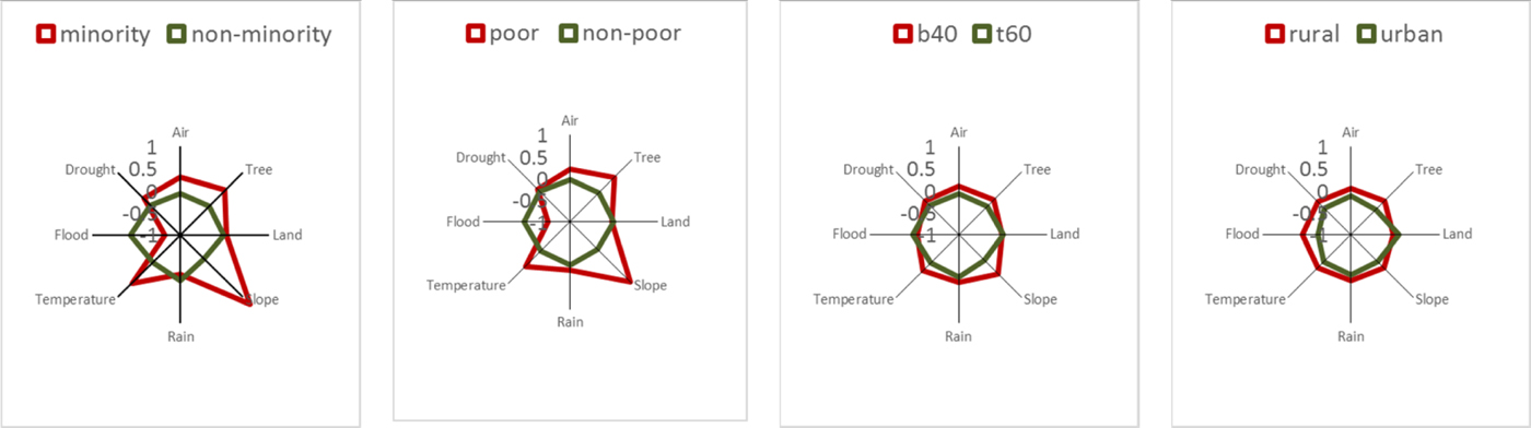
Figure 2. Environmental risk profiles across socio-economic groups in 2014.
5.2 Results
There are considerable differences in risk profiles between different groups. Households from ethnic minorities, those below the poverty line and those in the lowest two consumption quintiles live in much riskier communes (figure 2). It can be seen that the differences are most pronounced for the minority versus non-minority households. Poor households have a similar risk profile also because more than 50 per cent of poor households belong to ethnic minorities. Accordingly, households that face marginalization due to poverty or ethnicity are also disproportionally exposed to multiple, possibly interlinked, environmental risks.
For most environmental risks the differences between groups are significant. Ethnic minorities, poor households and those in the lowest two consumption quintiles face much higher air pollution, tree cover loss, steeper slopes, rainfall and temperature variability and drought hazards compared to their wealthier counterparts (table A.3). They are, however, exposed to lower flood hazards, confirming results from section 3 that flood risks are higher in more prosperous districts. These risk levels are very similar among groups in 2010, 2012 and 2014, suggesting that movement out of high risk zones has remained very limited over time (Narloch and Bangalore, Reference Narloch and Bangalore2016).
Looking at differences between rural and urban households, aside from land degradation, all other risk levels are much higher (table A.3) in rural households. Accordingly, the general risk profile is also more extreme for rural than urban households (figure 2). This finding is expected, as most of the ethnic minorities, poor households and those in the lowest consumption quintiles are rural households. Yet this finding does not imply that within rural or urban areas, poorer households are also more exposed than their wealthier counterparts, which will be further analyzed in the next section.
6. Risks and poverty within rural and urban areas
This section addresses the third research question (RQ3) which touches upon the last section to show whether the relationship between environmental risks at the commune level and household-level consumption levels is different between rural and urban areas.
6.1 Methods
The data is split into a rural and urban subsample to calculate correlation coefficients and run nonparametric analyses. For both sub-samples, the correlation coefficient between household-level consumption based on the expenditure data from the VHLSS 2014 and commune-level risks variables is calculated (table A.4). Households are further divided into consumption percentiles (100 groups) to show the mean level of consumption (x-axis) and of environmental risks (y-axis) for each percentile for the rural and urban sub-sample (figure 3).

Figure 3. Environmental risks across consumption percentiles within rural and urban zones in 2014.
6.2 Results
In both rural and urban areas, poorer households tend to live in communes with higher environmental risks. While for most environmental risks the correlation with per capita consumption is negative within rural as well as urban areas, the degree of correlation varies between rural and urban areas (table A.4). In rural areas, households in the lower percentiles are more exposed to air pollution, tree cover loss, steep slopes, rainfall and temperature variability, but less exposed to flood hazards (figure 3). In urban areas, poorer households are more concentrated in areas with high tree cover loss, slope, flood and drought hazards, while living in places with lower air pollution and temperature variability (figure 3).
Some remarkable differences emerge between rural and urban areas (figure 3 and table A.4). Poorer households seem to be less exposed to flood hazards in rural areas, but more so in urban areas. This finding could reflect the fact that many of the rural poor live in the mountainous areas where flood hazards are generally lower than in low-lying but wealthier river deltas and coastal zones, while many of the urban poor are pushed into high risk areas due to land constraints in the cities. This finding is consistent with a recent global analysis of flood exposure and poverty in 52 countries, which reports ambivalent results for flood exposure at the country level, but shows a strong signal of over-exposure of the poor when only focusing on urban areas (Winsemius et al., Reference Winsemius2015). Also poorer households are more exposed to air pollution and temperature variability in rural areas, but less in urban areas. Possibly, wealthier households live in rapidly developing urban areas with heavy traffic and industrial congestion, thereby being more exposed to air pollution.
7. Environmental risks and consumption differences and changes
To address the fourth research question (RQ4), this section investigates how environmental risks relate to consumption differences between households and consumption changes over time, applying a set of regression models. Notwithstanding several limitations, these analyses help provide first insights into the causal relationship between environmental risks and poverty.
7.1 Methods
Two sets of regression models are fitted to estimate the effect of environmental risks on consumption differences between households in the ‘Pooled’ cross-section and on consumption changes over time for the ‘Panel’ dataset. Using Ordinary Least Squares (OLS) estimators the following equation is fitted in the Pooled and Panel models:
 $$ {\bi Y}{_{i_{j_t}}} = {\bi \alpha} + {\bi \beta} {\bi R}_{{\bi j}} + {\bi \delta} {\bi Z}_{{\bi j}} + {\bi \omega} \ {\bi W}{_{j_t}} +{\bi \gamma} \ {\bi X}{_{i_{j_t}}} + {\bi \lambda} {\bi T}_{t} + {\bi u}{_{i_{j_t}}}, $$
where Y denotes per capita consumption observed for household i in commune j in year t (i.e., 2010, 2012, 2014) in the Pooled model and the change in per capita consumption for household i between years t (i.e., 2010–2012 and 2012–2014) in the Panel model. R measures the environmental risk profile in commune j, which is time-invariant, as described in section 2.2. β is the parameter of interest that indicates the consumption effect of environmental risks. Z includes commune-specific geo-spatial controls that do not change over time, such as proximity to cities and roads and the long-term average of rainfall and temperature. W includes a set of time-variant commune variables measured by rainfall and temperature levels in the survey years 2010, 2012 and 2014 for the Pooled model and by the change for 2010–12 and 2012–14 for the Panel model. X is a set of household-specific controls that vary over time, such as the levels of education, labor and land endowments in survey years for the Pooled model and the difference between years for the Panel model. X also includes time-invariant demographic characteristics, such ethnicity and gender.Footnote 13 T measures time-fixed effects to neutralize common trends over time. U is a random, idiosyncratic error term. The descriptive statistics of these variables are provided in table A.1.
A main concern when fitting models to estimate weather impacts on economic outcomes is endogeneity bias. Problems of reverse causation (e.g., high consumption growth in one place leading to environmental depletion) are minimized by taking the historic risk profile and not measuring actual environmental conditions in the survey years. Yet the model is likely to suffer from omitted variable bias caused by the potential correlation of risk variables with other commune characteristics that determine living standards.Footnote 14 To minimize omitted variable bias in this study, a set of observable commune characteristics is included that are likely to influence risk profiles and living standards, such as average rainfall and temperature conditions and distance from cities and roads. Nonetheless, to the extent that other, non-observable commune characteristics also determine risks and consumption, the estimates of β are biased. For instance, some communes may differ on the level of trust, which is likely to be associated with higher living standards and better environmental outcomes. In this case, our estimates would be biased upwards.
These regression models are estimated for various sub-samples to disentangle varying effects between groups, zones and years. For both the Pooled and Panel models, we first estimate the consumption effect one-by-one and then include all risk variables altogether. While only the results of the latter are presented, most of the results hold in the models with only one risk variable. Robust standard errors are estimated by clustering at the commune level in order to account for spatial correlation. For the Pooled model, the natural logarithm of per capita consumption is used in the regression to normalize the skewed distribution of consumption (i.e., many observations of low consumption levels and a few observations of very high consumption levels).Footnote 15
7.2 Results
Environmental risks are related to consumption differences between households. The results for environmental risks are presented in table 2, with the full results (including for all controls) shown in table A.5. Across all households from the Pooled cross-section, those households that live in communes with steeper slope, higher rainfall and temperature variability and flood and drought hazards have significantly lower consumption (table 2, column ‘All’). Only for land degradation does there seem to be a positive relationship, which may indicate communes of intensive agricultural expansion and growth, which could be positively associated to wealth in the short term. This finding points to possible estimation biases from unobservable factors, which do not allow us to establish clear, causal relationships with these data.
Table 2. The effect of environmental risks on consumption differences between ‘Pooled’ households in 2010, 2012 and 2014

Notes: This table indicates coefficients estimated from lsquo;Pooled' Cross-section model using Ordinary Least Squares. *0.10, **0.05, ***0.01 significance level. Values in parentheses indicate standard errors corrected for cluster correlation at the commune level. B40 denotes households in the bottom two consumption quintiles. Controls include current rainfall, current temperature, long-term rainfall, long-term temperature, distance city, distance road, area agriculture, area forest, area water surface, workforce, education, age head, female head, minority, year 2012, and year 2014. Full results (including for controls) presented in table A.5.
Source: Authors' calculation based on socio-economic data from VHLSS 2010, 2012 and 2014 and environmental data from Hansen et al., Reference Hansen2013; Vu et al., Reference Vu, Le and Vlek2014b; Brauer et al., Reference Brauer2015, Harmonized World Soil Database, Climate Research Unit, Bangalore et al., Reference Bangalore, Smith and Veldkamp2016, and Winsemius et al., Reference Winsemius2015.
Within the various groups, different risk factors matter for consumption levels. As differences in per capita expenditure between households below the poverty line are modest, it is not surprising that generally fewer variables are significant for the sub-sample of poor households and that the models have a much lower explanatory power (table 2, column ‘Poor’). The role of environmental risks in explaining consumption differences for households in the lowest two consumption quintiles follow the overall pattern, but there is a significant positive relationship with air pollution (table 2, column ‘B40’). The same finding emerges from the rural subsample (table 2, column ‘Rural’). Possibly rural households in communes closer to urban centers are wealthier, while being more exposed to air pollution than their counterparts in remote rural areas. Whereas in rural areas slope, rainfall and temperature variability and droughts are negatively related to consumption, in urban areas floods have a significant negative effect (table 2, column ‘Urban’), confirming the results in section 6. Very similar findings appear for the 2014 subsample, indicating that there are no considerable differences between the three survey years (table 2, columns ‘Urban 2014’ and ‘Rural 2014’).Footnote 16
Changes in consumption over time are only related to a limited number of risk variables and some show unexpected signs. The results for environmental risks are presented in table 3, with the full results (including for all controls) found in table A.6. Temperature variability relates to significantly higher consumption growth, mainly driven by urban households between 2012 and 2014 (table 3, columns ‘All’ and ‘Urban 2012–14’), while for households within the lowest two consumption quintiles, floods seem to have a positive effect on consumption growth (table 3, column ‘B40’). These effects can capture favorable weather conditions between 2010 and 2014 in these risk prone areas. For example, as long as no flood or extreme heat occurs, people living in flood plains or hotter zones can benefit from more profitable activities, such as floating rice or coffee cultivation. Higher land degradation is positively related to consumption growth in the rural subsample (table 3, column ‘Rural’). This effect may capture unobserved factors that facilitate higher consumption growth, such as non-farm income opportunities in more degraded areas.
Table 3. The effect of environmental risks on consumption changes over time of ‘Panel’ households in 2010–12 and 2012–14
Notes: This table indicates coefficients estimated from ‘Panel’ model using Ordinary Least Squares and differences over time for time-variant variables. *0.10, **0.05, ***0.01 significance level. Values in parentheses indicate standard errors corrected for cluster correlation at the commune level. B40 denotes households in the bottom two consumption quintiles. Controls include current rainfall, current temperature, long-term rainfall, long-term temperature, distance city, distance road, area agriculture, area forest, area water surface, workforce, education, age head, female head, minority, year 2012, and year 2014. Full results (including for controls) presented in table A.6.
Source: Authors' calculation based on socio-economic data from VHLSS 2010, 2012 and 2014 and environmental data from Hansen et al., Reference Hansen2013; Vu et al., Reference Vu, Le and Vlek2014b; Brauer et al., Reference Brauer2015, Harmonized World Soil Database, Climate Research Unit, Bangalore et al., Reference Bangalore, Smith and Veldkamp2016, and Winsemius et al., Reference Winsemius2015.
Yet a number of risk variables are related to lower consumption growth between 2010 and 2014, indicating a negative effect. Households in communes with higher PM2.5 concentration levels have a significantly lower consumption growth (table 3, column ‘All’). Lower consumption growth in 2012–14 is related to tree cover loss in rural zones and to rainfall variability in urban zones (table 3, columns ‘Rural 2012–14’ and ‘Urban 2012–14’). Among poor households, those living in communes with higher rainfall variability and drought hazards have a significantly lower consumption growth (table 2, column ‘Poor’), which is an alarming result suggesting that increasing rainfall variability and recurring droughts mainly have negative impacts on those that are already in a destitute situation.
Some interesting findings also appear from the results for the control variables (full results presented in tables A.5 and A.6). Higher levels of current rainfall and lower current temperatures are related to higher consumption levels and growth over time, which is broadly in line with the results in Narloch (Reference Narloch2016).Footnote 17 While larger distance to cities and roads relates to lower consumption levels as would be expected, it is related to higher consumption growth over time – possibly indicating a catching-up of more remote communes. Having access to larger agricultural and water surface areas has a positive effect on both consumption levels and growth over time. Ethnic minorities have lower consumption levels and also experience lower consumption growth when compared to wealthier households. However, within the sub-samples of households below the poverty line and in the lowest two consumption quintiles, ethnic minorities have higher consumption growth.
These results should be interpreted with some caution. First, based on the available data, omitted variable bias is minimized but not eliminated. As some of the findings suggest, there may be some incidences in which being located in a high risk zone can also indicate other factors that explain living standards but cannot be controlled for with the available data. Furthermore, it should be highlighted that some of the differences between the results from the Pooled and the Panel could be due to the different subsamples of households included in these analyses.
8. Conclusions
Despite several limitations related to the available data sets, this study provides important insights into the multi-faceted relationship between poverty and environmental risks based on the combination of high-resolution, geo-spatial data and household data from Vietnam. By using consistent data and methods within the same country, we can shed some light on how the relationship between poverty and multiple dimensions of environmental risk varies as a function of the channels through which poverty and risk interact. The findings highlight the fact that indeed the relationship is hard to generalize, as it depends on the specific types of risks, scale of analysis and locations of interest, and could possibly be driven by different causal linkages.
The main results regarding the four research questions are: (i) at the district level, the incidence of poverty is higher in high risk areas, (ii) similarly, at the household level, poorer households face higher environmental risks, (iii) for some risks, their relationship with household-level consumption varies between rural and urban areas, and (iv) environmental risks explain consumption differences between households, but less so consumption changes over time. In particular, lower household consumption levels are related to steeper slopes, higher rainfall variability and drought hazards in rural communes and higher flood hazards in urban communes. Consumption growth is lower for households in communes with higher air pollution. And for poor households, higher rainfall variability and drought hazards relate to lower consumption growth, implying the existence of poverty traps as relates to weather risks. Although the data do not allow us to conclude that environmental risks generally result in lower consumption growth, these findings suggest that poor people are disproportionally exposed to environmental risks.
More work is needed to confirm the potentially causal relationships between environmental risks and poverty. First, longer time-series data is needed to evaluate whether environmental conditions have long-lasting impacts on household living standards. Second, this study mostly relies on global datasets from remote sensing or modeling work, which need to be verified and refined with monitored data at the sub-national level – optimally from ground stations. Moreover, this study could only define historic risk profiles and not the actual environmental conditions and risk materialization within the survey years. The expansion of these analyses with such data will be an important area for deepening the findings of this work. Furthermore, alternative approaches could be applied to estimate causal impacts: for instance, to estimate deforestation-poverty linkages, future work may use discontinuities provided by borders (either at the sub-national or national level as in Crespo Cuaresma et al., Reference Crespo2017) or use instrumental variables such as temperature inversions (which have been used as an instrument for pollution levels as in Sager, Reference Sager2016).
Even in the absence of such analyses, some evidence already exists that shows the detrimental impacts of environmental risks on poverty and household welfare. An accompanying study, for example, shows that actual variation in rainfall and temperature conditions in rural areas is related to significant consumption and income effects also for poor people (Narloch, Reference Narloch2016). In addition, other work has shown the negative welfare and poverty impacts of flood and drought events (Thomas et al., Reference Thomas2010; Bui et al., Reference Bui2014; Arouri et al., Reference Arouri, Nguyen and Youssef2015). Moreover, poor people could be affected by environmental risks in many ways that go beyond income and consumption effects, such as detrimental health impacts or a decline in the quality of life due to poor environmental conditions. Such impacts cannot be measured with the available household data.
Altogether, the findings provide important insights into the relevance of poverty reduction policies under climate change. The disproportionate exposure of poor people to multiple environmental risks suggests that these people are more vulnerable to climate shocks. At the same time, climate change is likely to increase some of these risks, thus exacerbating already existing poverty traps. Strategies to reduce poverty – especially in rural areas – need to address environmental risks and climate change simultaneously. For example, ecosystem-based adaptation could strengthen ecosystem resilience to climate change and reduce environmental risks, while improving the livelihoods of people depending on these ecosystems. Carefully designed land-use planning policies, paired with investments in livelihood support and improved mobility that encourage resettlements and avoid new settlements in high risk areas, are another strategy to reduce exposure to environmental risks and climate shocks, while reducing human pressure on already fragile ecosystems. Generally, addressing environmental risks deserves greater attention in poverty reduction policies – especially in the face of climate change.
Supplementary material
The supplementary material for this article can be found at https://doi.org/10.1017/S1355770X18000128
Acknowledgements
This work is part of programmatic work on Climate Change, Poverty and Climate Resilience in Vietnam and was developed under the oversight of Christophe Crepin and Stephane Hallegatte. We are very thankful to the World Bank Vietnam team for providing the Vietnam Household Living Standards Survey (VHLSS) data and to Linh Hoang Vu and Ha Thi Ngoc Tran for helping with data questions. We very gratefully acknowledge data received from Vu Manh Quyet (on land degradation) and data processed by Joseph Muhlhausen (on air pollution). Very helpful suggestions were received from Diji Chandrasekharan Behr and two anonymous reviewers. Mook Bangalore gratefully acknowledges financial support by the Grantham Foundation for the Protection of the Environment and the UK's Economic and Social Research Council (ESRC).


