1. INTRODUCTION
Laser ablated plumes created with nanosecond lasers operating at fluences of a few J/cm2 are of relevance to pulsed laser deposition of new technological materials (e.g., Chrisey & Huler, Reference Chrisey and Hubler2003; Eason, Reference Eason2006) as well as for other applications such as laser induced breakdown spescopy (e.g., Godwal et al., Reference Godwal, Tascuk, Lui, Tsui and Fedosejevs2008; Schade et al., Reference Schade, Bohling, Hohmann and Scheel2006). There has naturally been a great interest in understanding the dynamics of such plumes and several model approaches have been presented (e.g., Farnsworth, Reference Farnsworth1980; Kelly & Dreyfus, Reference Kelly and Dreyfus1988; Singh & Narayan, Reference Singh and Narayan1990; Aisimov et al., 1993). To this end, several diagnostic techniques, such as laser induced flurcence, interferometry, plasma imaging, probes, and particle measurements have been employed (Dreyfus, Reference Dreyfus1991; Doyle et al., Reference Doyle, Martin, Al-Khateeb, Weaver, Riley, Lamb, Morrow and Lewis1998; Martin et al., Reference Martin, Doyle, Al-Khateeb, Weaver, Riley, Lamb, Morrow and Lewis1998; Doggett & Lunney, Reference Doggett and Lunney2009; Caridi et al., Reference Caridi, Torrisi, Margarone and Borrieli2008).
Recently, we have added to this diagnostic capability by employing Thomson scattering (Delserieys et al., Reference Delserieys, Khattak, Pedregosa Gutierrez, Lewis and Riley2008a, Reference Delserieys, Khattak, Lewis and Riley2009). This is a powerful technique that has been widely used in fusion plasmas as well as high temperature laser-plasmas, and electrically driven RF plasmas and more recently, as a proposed method for production of short X-ray bursts (e.g., Liu et al., Reference Liu, Xia, Liu, Wang, Cai, Wang, Li and Xu2010, and references therein). Apart from early preliminary work (George et al., Reference George, Englehar and DeMichelis1970; Izawa et al., Reference Izawa, Yamanaka, Tsuchimori, Onishi and Yamanaka1968, Reference Izawa, Yokoyama and Yamanaka1969), it has not been used very extensively in low temperature plumes of the sort investigated here. In previous work (Delserieys et al., Reference Delserieys, Khattak, Pedregosa Gutierrez, Lewis and Riley2008a, Reference Delserieys, Khattak, Lewis and Riley2009), we used KrF laser radiation to generate the plume. Our principal findings were that an isothermal model of expansion fitted the data better than an isentropic model (Delserieys et al., Reference Delserieys, Khattak, Lewis and Riley2009; Stapleton et al., Reference Stapleton, McKiernan and Mosnier2005). By observing the power law of decay for electron and atomic densities, we concluded that di-electronic recombination was a significant factor in the plume evolution over the first microsecond after ablation. Furthermore, we concluded that the plasma created was very effective in screening the solid from the laser; with photo-ionization being a strong absorption process in the plume. In this new work, we have used a second harmonic Nd:YAG (532 nm) laser to create the plume. As will be seen below, some of the conclusions are similar to those for KrF ablation, whilst others are not.
2. EXPERIMENTAL SET-UP
As in the previous work, we used a synchronized laser at 532 nm as the Thomson scattering probe. By using a gated intensified charged coupled device (ICCD) camera, we were easily able to distinguish scattering from the probe and pump pulses. The system used in the experiment is shown schematically in Figure 1. This set-up enabled monitoring of the temporal and three-dimensional (3D) spatial evolution of the ablated plasma, assuming symmetry about the main expansion axis. Two 10 Hz Nd:YAG lasers operating in the second harmonic regime were used for both ablation and probing of the plasma plume. In vacuum (10−4 mbar), a rotating Mg target was ablated by an 8 ns pulse focused to about 1 mm full width at half maximum spot at fluence of about 13.5 J/cm2. At a controlled delay time (200–1000 ns), a separate, 7 ns laser pulse of energy about 230 mJ, focused down to a 0.4 mm spot, probed the plume in a direction parallel to the target surface and normal to its principal expansion axis. The scattered signal was collected at 90° where the scattered power is maximum. Using a set of collecting optics, the scattered photons were imaged onto the entrance slit of an imaging double grating spectrometer (SPEX 750, 1200 l/mm, dispersion 5.7 Å/mm) which had a gated ICCD as a detector. This enabled 1:1 imaging of the plume onto the spectrometer entrance slit with the direction of spatial resolution (along the slit length) corresponding to the lateral direction across the plume i.e., along the path of the probe. Spatial profiling in the axial direction was achieved by changing the target's position relative to the probing beam from 2 to 4.5 mm with a step of 0.5 mm; the width of the slit (100 µs) sets the spatial resolution in the axial direction. The plasma evolution was monitored on a time scale of 200–1000 ns. Each image is an accumulation of about 400 laser shots, each gated for 20 ns. The data was corrected for the plasma self emission, the stray light and background signal. The greatest challenge in setting up the experiment is stray light reduction (Warner & Heiftje, Reference Warner and GM Hieftje2002) so great care was taken in equipping the chamber with baffles and light traps. The efficiency of the entire system was calibrated by measuring the Rayleigh scattering from 10 mBar of Ar fill in the chamber (Sneep & Ubachs, Reference Sneep and Ubachs2005). This allowed absolute electron densities to be determined from the intensity of the scattered signal. The data collected is characterized by the scattering parameter α, where α = (kλD)−1, k is the scattering wave-vector and λD is the Debye screening length. The spectra collected at 13.5 J/cm2 all showed values of α < 1 and thus described the non-collective regime, as can be seen in Figure 1, which shows a sample Thomson scattering spectrum taken 2 mm from the target surface and at 200 ns delay after ablation.

Fig. 1. (Color online) (a) Left: Schematic of experimental arrangement. (b) Sample Thomson spectrum taken at 2 mm from target surface and 200 ns delay. Fits to the spectra allow spatio-temporal maps of the electron density and temperature to be constructed.
3. RESULTS
In Figure 2, we can see time histories of the electron density and temperature for the case of 13.5 J/cm2 and 2–4.5 mm from the target surface. With the earlier KrF data (Delserieys et al., Reference Delserieys, Khattak, Pedregosa Gutierrez, Lewis and Riley2008a, Reference Delserieys, Khattak, Lewis and Riley2009), which used a similar fluence of about 10 J/cm2, we found that the electron density could be fitted to about t −5 scaling, much faster than the t −3 scaling expected for a simple 3D expansion of an initially uniform slab of plasma, and this more rapid decay was deduced to be a result of di-electronic recombination occurring about 250 ns timescale. For the new data presented here, using 532 nm laser radiations, we see that the rate of fall for the electron density is much slower. Analysis of the expected recombination rates indicates that for the peak electron density of 1.3 × 1015 cm−3 and temperature of 0.91 eV for the case 2 mm from the target, the di-electronic recombination time is of the order of 60 µs (Altun et al., Reference Altun, Yumak, Badnell, Loch and Pindzola2006). For radiative and three-body recombination (e.g., Thum-Jaeger et al., Reference Thum-Jaeger, Sinha and Rohr2000), even for excited states the rates are significantly longer than the 1 µs duration of the experiment. Looking at Figure 2, we can see that the electron temperature decays more slowly than the isentropic expansion dependence of t −2. This may be due to re-heating of the electrons by 3BR; this can occur despite the recombination rate being relatively slow (Rumsby & Paul, Reference Rumsby and Paul1974) because the temperature is small compared to the ionization potential and the energy transfer per recombination is on average of about I p + 1.5 kT e. For the electron temperature and density at 2 mm and 200 ns delay, the timescale for recombination to the ground state is about 20 µs and the rate of heating of the free electrons would be expected to be on the order of 0.5 eV/μs.

Fig. 2. (Color online) Temporal evolutions of the electron density and temperature in laser ablated Mg at 2–4.5 mm distance from the target surface. For the case of 2 mm from target surface, we show results from earlier work on KrF as a comparison.
We can further investigate the degree of recombination during the observed phase of expansion by following a specific volume of the plasma by assuming a self-similar expansion where the volume of plasma is expected to have a constant velocity. This is a reasonable assumption; starting long after the pulse has finished and at 2 mm from the surface, where 3D expansion has been established. Thus, for example, the volume of plasma probed at 400 ns and 2 mm can be assumed to be expanding with an axial velocity of 5 × 105 cm/s. Thus, it will appear at 2.5 mm at 500 ns delay and so on until it reaches 4.5 mm at 900 ns. We have electron density measurements at all the appropriate times and distances and these are shown in Figure 3, where we also show the more limited data set for the plasma that appears at 2 mm at 200 ns delay and is assumed to travel at 106 cm/s and so appears in two other data points. In each case, the time dependence of the electron density decay can compared to a t −x power law and best fit values for x = 2.2 and x = 2.6 are obtained. However, we can see in the figure that a fit to t −3, corresponds very well to the data. In principle, the finite size of the focal spot will affect the expansion rate, but analysis using simple hydrodynamic models (see below) indicates the effect is limited for our dimensions, with x = 2.9 expected.

Fig. 3. (Color online) Temporal evolution of the electron density for plasma slices reaching 2 mm in 200 ns and 400 ns; fitted to t −x power law dependencies.
4. RAYLEIGH SIGNAL
The picture becomes a little more complex if we look at the Rayleigh scattered signal as a function of time. We see, in Figure 4, the measured signal for 2–3.5 mm. Data for 4 mm and 4.5 mm follows the same trend, but with much lower intensity. What is striking is that the Rayleigh signal rises with time rather than falling. We can understand this from considering the Rayleigh scattering cross sections for atoms and ions. For the former, in the ground state, it is calculated to be 4.15 × 10⁻²⁶ cm2/sr for 90° scatter, while it is 0.98 × 10⁻²⁶cm2/sr for Mg+ in the ground state (Delserieys et al., Reference Delserieys, Khattak, Sahoo, Gribakin, Lewis and Riley2008b). For Mg2+, we have used a measure of the polarizability (Bockasten, Reference Bockasten1956) to calculate a cross section of 8.45 × 10⁻³⁰ cm2. We do not expect higher ionization stages as the ionization potential of Mg2+ is about 80 eV. For excited states of the neutral atom, the Rayleigh scattering is even larger, for example, the metastable 3s3p 3P term for Mg I, observed via Raman satellites in earlier work with KrF ablation, has a cross section of 3.15 × 10⁻²⁴ cm2/sr (Delserieys, Reference Delserieys, Khattak, Sahoo, Gribakin, Lewis and Riley2008b); although, the absence of Raman satellites in the present work indicates a small population for the metastables. The implication of the temporal rise of the signal in Figure 4, is either that, recombination to more strongly scattering neutrals is occurring or that the plasma is becoming less ionized at a given point in space as the plasma passes by. The electron density data above suggests that the latter is the proper explanation. We can further investigate this by taking the same volume elements of plasma probed in Figure 3 and looking at the Rayleigh scatter signals, which are plotted for these volume elements as a function of time in Figure 5.

Fig. 4. (Color online) Rayleigh scattered signal as a function of time at 2–3.5 mm from the target surface; the lines are only to guide the eye.

Fig. 5. (Color online) Temporal evolution of the Rayleigh peak for plasma slices reaching 2 mm in 200 ns and 400 ns fitted to t −x power law dependencies.
This shows the signal decreasing approximately as t −2 and t −2.7. For the faster element with only three data points, this is not in very good agreement with simple 3D expansion but for the slower element with more detailed data, the decay is in much better agreement. For this element, the good agreement with the t –3 power law supports the claim that recombination does not play a significant role, and that the decay is mainly governed by volumetric expansion. We can note that if we estimate the number density of the neutrals and fit that with time, we get a t −2.9 dependence. This exactly as expected when given the effect of the finite spot size, which leads to slightly non-3D expansion, especially close to the target surface.
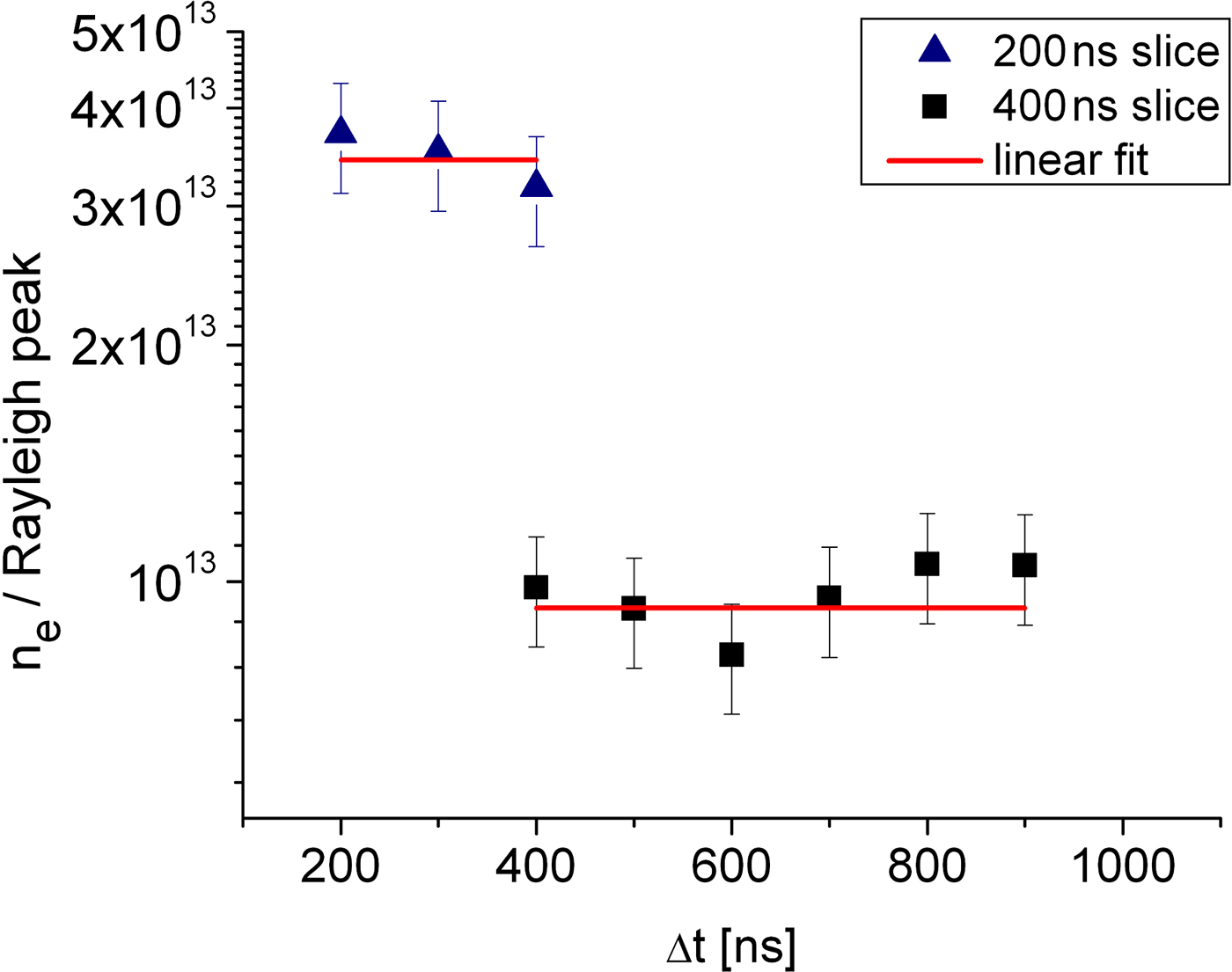
We can further support this thesis by plotting a ratio of the measured electron density to Rayleigh signal for the same plasma volumes. This is shown in Figure 6. (Note that we do not simply plot the electron feature signal divided by Rayleigh signal, as the electron feature depends on the scattering parameter, α, as well as on density.) If both signal decays are purely from expansion, we might expect a constant ratio i.e., a straight horizontal line. If recombination is occurring the decrease in electron density should go hand in hand with an increase in the Rayleigh signal (since atoms scatter more than ions) and a drop in the ratio should occur with time. There is a slight drop in the faster volume element but in both cases, within the error bars, a constant ratio fits the data. We note that the ratios presented here should link to the average ionization of the plasma volumes. We expect that the faster plasma volume, with its higher ratio of electron density to Rayleigh signal, represents a higher average ionization.

Fig. 6. (Color online) Ratio of the electron density and Rayleigh peak for plasma slices arriving at 2 mm in 200 ns and 400 ns, good agreement to a constant ratio indicates the absence of recombination in the plume.
We estimate the average ionization in the two plasma volume elements in the following way. For each data point we have a measure of the electron density. We also have a measure of the Rayleigh signal and know the cross-sections for the different ion stages. For a collisional radiative equilibrium, we know that for the typical densities of our experiment, the neutrals are not expected to exist alongside Mg2+ ions in the same plasma volume. Thus, making an initial assumption, for the slower element, that there are no Mg+2 ions we can set the ion density equal to the electron density and deduce the contribution of ions to the Rayleigh signal, assigning the rest to neutral atoms and a small contribution from the Thomson scattering ion feature, allowing an estimate of Z*. As can be seen in Figure 7 the value of Z* is basically constant for this plasma element, even indicating a slight rise, although this is smaller than the error bars. The value of Z* being about 0.7 gives us some justification post-priori that our assumption of no doubly ionized ions is valid. For the faster volume element, with a higher ionization, making the assumption of no Mg2+ ions leads to a negative value for the neutral density. Thus we try the opposite and assume the plasma is made of Mg+ and Mg2+ ions with very few neutrals. This leads to estimated average ionization of about 1.4 as seen in Figure 7. The large error bars for the faster plasma volume are due to the very small value of the Rayleigh scattering cross section for Mg2+.

Fig. 7. Z* evolution of plasma slices reaching 2 mm in 200 ns and 400 ns.
The preceding analysis of ionization depends on the assumption that Mg I and Mg III do not generally co-exist in the plasma. An LTE analysis indicates that, for electron densities in the 1014–1018 cm−3 range, Mg I and Mg III only have comparable densities when both are small compared to the number of Mg II ions. The fact that significant ionization is measured for the plasma elements when, for much of their history, the electron temperature is less than 0.5eV indicates that some “freezing” of ionization is occurring. What this means is that the ionization balance is established at some higher density hotter phase and as the plasma rapidly expands to low density the recombination mechanisms are not rapid enough for the ionization balance to reflect the lower temperature (e.g., Riley et al., Reference Riley, Weaver, Morrow, Lamb, Martin, Doyle, Al-Khateeb and Lewis2000).
5. COMPARISON WITH ANALYTICAL MODELS
Comparison of the data for 532 nm ablation has been made with analytical expansion models that assume the plasma expands in three dimensions either isentropically or isothermally (Singh & Narayan, Reference Singh and Narayan1990; Anisimov et al., Reference Anisimov, Bauerle and Luk'yanchuk1993; Stapleton et al., Reference Stapleton, McKiernan and Mosnier2005; Afanasiev et al., Reference Afanasiev, Isakov, Zavestovskaya, Chichkov, Von Alvensleben and Welling1999). The results depend on several parameters that must be decided upon. These are (1) the axial and lateral expansion velocities, (2) ionization degree; since the model calculates atomic/ionic density and the scatter determines electron density, and (3) the mass in each ablated plume. For (1), we have measured the lateral expansion of the plasma edge from observing the extent of the scatter signal in the spatially resolved data and found it to be about1.4 × 106 cm/s at the plasma edge. Analysis of the electron density contours for different distances from target surface indicate that the ratio of axial to lateral expansion velocity to be about 2, which is typical for this spot size (Martin et al., Reference Martin, Doyle, Al-Khateeb, Weaver, Riley, Lamb, Morrow and Lewis1998; Doggett & Lunney, Reference Doggett and Lunney2009) and our edge velocity is 2.5 × 10⁶ cms−1 that is consistent with low density plasma being observed at 4.5 mm from the target at 200 ns. The ablated mass was measured by firing 500 shots onto a single spot and measuring the crater left; the ablated mass per shot was estimated to be 8 × 10⁻⁸ g. This may be an upper limit as some mass may be lost long after the initial ablation event as heat conduction allows a slowly evaporating molten pool to be created beneath the initially ablated layer. This measured ablated mass is in fact more than 20 times smaller than would be expected from a simple model (Amoruso et al., Reference Amoruso, Bruzzese, Velotta and Spinelli1999) and indicates that there is likely to be either strong reflection of the laser from the critical surface or strong screening in the plasma plume, thus decoupling the energy from the solid and reducing ablation. This phenomenon has been noted previously (Lunney, Reference Lunney1995). For the ionization, we noted experimentally that this is not spatially uniform and so we use a “typical” value of Z* = 1 and will discuss the possible implications of this approximation later.
Comparing isothermal and isentropic models we see, in Figure 8 that an isothermal model fits moderately well if we take the ablated mass to be 8 × 10⁻⁸ g, as measured. An isentropic model fits only if the ablated mass is reduced by a further factor of >10, well below the measured value. This, we think, tends to indicate that an isothermal model of the plume fits better than an isentropic model. Changing the assumed ionization between, for example, 0.7–1.4 will not alter this conclusion significantly. Even for the isothermal case, however, we note that agreement is not so good at early time. This is a feature for all distances from the target surface- at early time the data gives density lower than the model. We see, in Figure 9, that the spatial temperature profile broadly supports an isothermal model at later times but at very early times does not.

Fig. 8. (Color online) Comparison of experimental electron density at d =2 mm (left) and d = 4 mm (right) with various assumptions. The assumption of isothermal expansion clearly fits best to the measured electron densities.
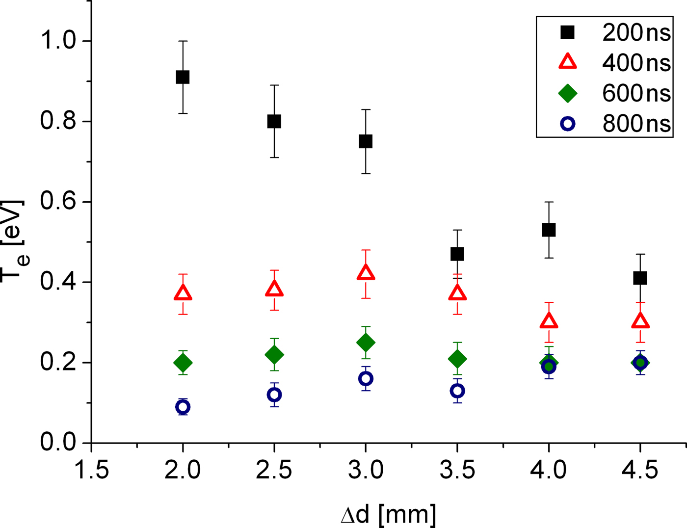
Fig. 9. (Color online) Experimental spatial profile of electron temperature at 200 ns (squares), 400 ns (triangles), 600 ns (diamonds), and 800 ns (circles).
In Figure 10, we compare the models and data at fixed times as a function of distance from target. We can see here that, for either model, the shape of the profile does not match well with experiment, except at late times when both are relatively flat. These mismatches between the self-similar expansion models and data may have several causes. One significant cause could be the already mentioned density, ionization and temperature gradients in the initial plume just after the end of the laser pulse. We should consider that for self similar expansion to be truly valid we expect the initial density profile to match the late time profile. For the isothermal case in particular, this is problematical as, in principle there is no definite edge to the plasma. However, it has been argued (e.g., Pert, Reference Pert1980) that if the expansion is isothermal, the initial density profile will ultimately take on the Gaussian form expected for self-similar isothermal flow. Another cause may arise from the finite (0.4 mm) width of the probe beam. At early time, closer to the target surface, the probe samples a larger fraction of the plume in the radial direction than for later times and further from the target. A consequence of this is that the outer, lower density part of the beam plays a more significant role and the average density sampled may be reduced from the true axial peak. However, a quick estimate based on lateral velocity indicates that, at 200 ns and 2 mm from the target surface, the spatial scale of the lateral expansion is on the order of about 3 mm. This is somewhat larger than the radius of the probe and lateral averaging thus would appear to be an unlikely cause of the disagreement.

Fig. 10. (Color online) Comparison of experimental electron density at t =200 ns, t = 400 ns, and d = 800 ns to (a) isothermal expansion model and (b) isentropic expansion model; with Z* = 1 and different ablated masses.
Finally, one aspect not accounted for in the simple modeling is the profile of the focal spot of the laser, which for the laser used was approximately Gaussian. In principle this should affect the ratio of the lateral to transverse velocities. It was reported by Kumar et al. (Reference Kumar, George, Singh and Nampoori2010) that a Gaussian profile in fact led to a more highly directed plume than a top hat profile as assumed in the model. These velocities are however, in our case, measured experimentally and input to the model. In addition, we have used the experimentally determined ablated mass in the simulation.
6. CONCLUSIONS
We have used Thomson scattering to study the spatial and temporal evolution of an Mg laser produced plasma generated with 532 nm radiation. The density profiles do not fit well to simple models. However, the data does allow us to come to some conclusions. First, as with KrF ablation, we found that the isothermal model fits the experimental data better. This conclusion is based primarily on measuring the spatial temperature profiles axially and the estimates of ablated mass per shot made experimentally. The measured ablated mass per shot suggests that ablation from the solid surface is severely inhibited; probably due to a combination of reflection and absorption in the plasma cloud above the surface. Second, unlike the KrF case we do not see strong evidence of recombination in the plume. On the contrary, following individual plasma volume elements in the evolution of their electron density, Rayleigh signal and average ionization, agrees well with expected simple 3D expansion. On the other hand, we do see a strong axial spatial gradient in the ionization of the plasma plume. This is likely to be a result of strong gradients in the plasma present just after the laser irradiation is over and before free expansion begins. These gradients may explain the poor fit of axial spatial profiles to simple models. To get a better understanding of the data we need to consider the details of the dynamics of the laser ablation process close to the target surface and during the pulse. (e.g., Chen et al., Reference Chen, King, Hes, Leboeuf, Geohegan, Wood, Puretzky and Donato1999). In particular, the effect of wavelength on the degree of coupling to the target and role of processes such as photo-ionization in the dense plume. For our present work, we do not probe that regime for a variety of practical reasons, including refraction and absorption of the beam at high density and limitations on spatial resolution.
ACKNOWLEDGMENT
One of the authors, EN, is supported by an overseas research studentship from the Queen's University of Belfast.