


1. INTRODUCTION
In the general context of a direct drive inertial confinement fusion (ICF) experiment, proper understanding of energy (heat) transport in dense plasma (i.e., following laser irradiation of a solid) is of crucial importance. It indeed influences several aspects of ICF like laser absorption, X-ray emission, hydrodynamic efficiency, implosion dynamics, ablation front stability, and symmetry. Such understanding is however still limited nowadays. As it was observed already a few decades ago, the standard Spitzer-Harm (S-H) theory for plasma heat transport (Spitzer & Harm, Reference Spitzer and Harm1953), derived in the limit of small temperature gradients, cannot adequately reproduce actual observations. Instead it was found that one needs to limit artificially the predicted heat flux. In practice, the actual heat flux is limited to only 3 to 10% of the free streaming value, depending on the experimental conditions and measurements (Young et al., Reference Young, Whitlock, Decoste, Ripin, Nagel, Stamper, Mcmahon and Bodner1997; Mead et al., Reference Mead, Campbell, Estabrook, Turner, Kruer, Lee, Pruett, Rupert, Tirsell, Stradling, Ze, Max and Rosen1981; Hauer et al., Reference Hauer, Mead, Willi, Kilkenny, Bradley, Tabatabaei and Hooker1984) and has even been found to be time dependent (Regan et al., Reference Regan, Epstein, Goncharov, Igumenshchev, Li, Radha, Sawada, Seka, Boelhy, Delettrez, Gotchev, Knauer, Marozas, Marshall, Mccrory, Mckenty, Meyerhofer, Sangster, Shvartz, Skupsky, Smalyuk and Yaakobi2007). This points to the obvious lack of predictability of such S-H model. The cause behind heat flux inhibition is generally attributed to two competing mechanisms: the non-locality of the heat carrying electrons (Luciani et al., Reference Luciani, Mora and Pellat1985; Epperlein et al., Reference Epperlein, Rickard and Bell1988; Schurtz et al., Reference Schurtz, Nicolai and Busquet2000), which arises when the thermal gradient length is lower than a few electron mean free paths, and the reduction of this mean free path due to Larmor gyration (Braginskii, Reference Braginskii and Leontovish1965) around the toroidal magnetic fields generated in the plasma parallel to the target surface (Stamper et al., Reference Stamper and Ripin1975). Furthermore, thermo-electrical effects associated with magnetic field can rise, depending on the geometry.
In order to assess the weight of these two counter-acting effects, an experiment was recently performed using the Ligne d'Integration Laser facility (Schurtz et al., Reference Schurtz, Gary, Hulin, Chenais-Popovics, Gauthier, Thais, Breil, Durut, Feugeas, Maire, Nicolai, Peyrussse, Reverdin, Soullié, Tikhonchuk, Villette and Fourment2007), in which the heat flow velocity through a plastic target illuminated by 0.35 µm light at ≈1015 W·cm−2 was measured. The target was planar and the focal spot was a smoothed Gaussian obtained by combining longitudinal spectral dispersion with focusing gratings and continuous-phase plates.
To interpret that experiment, the measurements were compared with simulations performed using the two-dimensional (2-D) hydrocode CHIC (Maire et al., Reference Maire, Abgrall, Breil and Ovadia2007) and showed that multi-dimensional effects are also to be taken into account to properly understand heat flow. The radial fluxes determine the electron temperature at the laser axis and thus the longitudinal heat flow. As a consequence, the non-local effect acts to inhibit the radial flux and therefore increase the axial temperature and the longitudinal flow. On the contrary, the magnetic fields increase the radial flux via the Righi-Leduc effect, which rotates the heat flow, and thus reduces the longitudinal heat flow. The experimental results were well reproduced by the simulations only when the magnetic fields were taken into account. This hinted at the predominant role played by magnetic fields in 2-D heat flows, but during this experiment no direct measurement of the magnetic map was performed.
Measurements of magnetic fields in high density plasmas are nowadays possible with the help of energetic proton radiography (Mackinnon et al., Reference Mackinnon, Patel, Town, Edwards, Phillips, Lerner, Price, Hicks, Key, Hatchett, Wilks, Borghesi, Romagnani, Kar, Toncian, Pretzler, Willi, Koenig, Martinolli, Lepape, Benuzzi-Mounaix, Audebert, Gauthier, King, Snavely, Freeman and Boehlly2004). In these conditions, magnetic fields arise due to crossed temperature and density gradients in the plasma expanding toward vacuum. The radiography technique allows accessing regions not attainable by optical probes, and is a unique tool to retrieve time and space-resolved information on the actual field structure, even in dense, solid plasmas. The proton imaging technique is based on the deflections undergone by protons as charged particles when crossing a zone where electric and/or magnetic fields are present by the protons being subsequently projected onto a film-detector, it allows retrieving, from the film, an image of the topology of these fields and information about their amplitude. In particular, the existence and nature of magnetic fields self-generated in dense plasma, produced by a ns laser irradiation of a planar solid target, was demonstrated at RAL laser facility (Nilson et al., Reference Nilson, Willingale, Kaluza, Kampediris, Minardi, Wei, Fernandes, Notley, Bandyopadhayay, Sherlock, Kingham, Tatarakis, Najmudin, Rosmuz, Evans, Haines, Dangor and Krushelnick2006; Cecchetti et al., Reference Cecchetti, Borghesi, Fuchs, Schurtz, Kar, Macchi, Romagnani, Wilson, Antici, Jung, Osterholtz, Pipahl, Willi, Schiavi, Notley and Neely2009) using ultra-intense laser produced protons and at the Omega facility of Rochester (Li et al., Reference Li, Seguin, Frenje, Rygg, Petrasso, Town, Amendt, Hatchett, Landen, Mackinnon, Patel, Tabak, Smalyuk, Sangster and Knauer2006) using mono-energetic (14.7 MeV) protons.
Some of these studies pointed to field evolution and expansion mechanisms dominated by fast advection that are not thoroughly explained by present days magneto-hydrodynamic theory and associated numerical models. In particular, the Nernst velocity was suspected to play a major role in the evolution of these fields (Willingale et al., Reference Willingale, Thomas, Nilson, Kaluza, Bandyopadhyay, Dangor, Evans, Fernandes, Haines, Kampediris, Kingham, Minardi, Notley, Ridgers, Rosmuz, Sherlock, Tatarakis, Wei, Najmudin and Krushenick2010). In order to contribute to the understanding of the physical processes involved in the evolution of these fields and of their influence on the heat wave propagation, we performed an experiment, reported here, devoted to measure for the first time the heat flow and the self generated magnetic fields simultaneously. The experiment was performed on the LULI 2000 laser facility.
2. EXPERIMENT SETUP
2.1. Nanosecond Interaction Beam
A nanosecond pulse was used to drive heat flow in a solid target (see Fig. 1a, 1b). The heat flow was characterized by time-resolved spectroscopy. A synchronized short pulse was used to produce the proton beam devoted to measure the magnetic fields in the plasma (see Fig. 1b, 1c). In order to explore different 2-D geometries, two phase plates were used to shape different focal spots of the long pulse. The main LULI 2000 beam, frequency-doubled at a wavelength λo = 526 nm, was focused using a f/4 lens onto a composite target with an angle of 32.5° from the normal incidence (see Fig. 1a), with an energy varying from ~200 to ~400 J. The pulse “top-hat” temporal length was varied between 2 and 5 ns so to be able to achieve on target intensities from 1 to 3 × 10¹⁴ W/cm2, representative of the conditions of the ablator of a gain target (Atzeni et al., Reference Atzeni, Schiavi and Bellei2007).

Fig. 1. (Color online) (a) Experimental Setup top view. The LULI2000 ns laser beam is focused at 32.5° on the interaction target. On the specular reflection direction a high reflectance target is placed to infer the absorbed laser energy. A crystal spectrometer coupled to a streak camera in the X-domain is used to measure the emission of X-rays from tracers buried in the target and to resolve it temporally. The Pico2000 laser beam is focused on a gold target to produce the proton beam for proton radiography of the fields developing on the illuminated face of the interaction target. Proton deflections are recorded on a stack of Radiochromic films positioned along the normal to the interaction target. The inset shows a typical spectrum of the accelerated proton beam. (b) Heat flux measurement principle: interaction of the ns pulse with the composite target. (c) B-field measurement principle.
The focusing at an angle caused the focal spot profile to be projected onto the target with an elliptical shape of aspect ratio, minor/major axis ≃0.84. Two focusing configurations were used for the long pulse, where the magnetic fields were favored or inhibited close to the laser propagation axis, by the use of different phase plates. Together with laser pulse energy and duration measurements performed on every shot, the focal spots characterization allowed retrieving the actual intensity map on target for the long pulse incidence angle. For both phase plates, the laser intensity map at the target position was measured (in a plane transverse to the laser axis) by an optical imaging system during non amplified shots. Using a phase zone plate (PZP), (Stevenson et al., Reference Stevenson, Norman, Bett, Pepler, Danson and Ross1994) we obtained at the target position, i.e., 600 µm beyond the focal plane of the focusing lens, a 200 µm diameter plateau (super-Gaussian of order 5) surrounded by wings presenting a Gaussian profile with 500 µm full width at half maximum (FWHM). The energy balance between the plateau and the wings was 53% and 47%, respectively. The intensity distribution for the PZP phase plate was also characterized at full laser energy by firing a shot on a 22.5 µm aluminum foil and measuring the shock breakout time with a streaked optical imagery. For such a well known material, a comparison between the measured breakout time and a hydrodynamical simulated one, where the laser intensity was a free parameter, confirmed the validity of the calculated intensity on target. The second phase plate was a random phase plate (RPP) (Kato et al., Reference Kato, Mima, Miyanaga, Arinaga, Kitagawa, Nakatsuka and Yamanaka1984) shaping a 95 µm FWHM Gaussian spot with 66% energy surrounded by 300 µm FWHM Gaussian wings. Error bar on laser intensities was ±10%, deduced from the uncertainties on laser energy and duration measurements together with the shock breakout calibration on aluminum foil.
2.2. Long Pulse Absorption
In order to complete the energetic characterization of the interaction, a scattering reflectance plate (SPECTRALON brand) of 30 × 30 cm2 was placed on the specular reflection of the incident beam (see Fig. 1c) about 60 cm away from the target, in order to evaluate, through diffuse reflection, the energy that was reflected from the target and deduce the amount of absorbed energy within the target itself. The analysis of the scattered energy indicated that, for various pulse lengths, about 90% of the energy was absorbed, in good agreement with numerical evaluations (details of the hydrodynamic code used for this purpose will be given later).
2.3. X-ray Imaging
An X-ray pinhole camera (PHC) imaged the target plane. It was placed at an angle of 45° with respect to the incidence plane (defined by the laser direction and the target normal) and 32.5° with respect to the target normal. The PHC recorded time-integrated images of the X-rays emitted by the target, filtered by a 6 µm thick aluminum foil. The detector was an image plate. Image magnification was 12.6 ± 0.1, and the resolution, given by the pinhole diameter, was 30 µm. Images were treated by compensating the distortion due to the angles of view of the imaging system with respect to the target plane. Uncertainty on the magnification due to alignment was taken into account. The background noise was then removed. Despite the focal spot projection on target being an ellipse, due to the angle of incidence, we found nearly perfectly circular X-ray spots, with an ellipticity of 1.02 ± 0.08. Measurements showed that the original elliptical intensity profile of the laser spot on target was lost, suggesting that the plasma expansion was quicker along the smaller axis direction resulting in a symmetrization of the global expansion. Images of the emission were fitted by Gaussian profiles for the RPP and PZP focal spot interaction. Interaction with the PZP profile produced emission spots in the 240–300 µm FWHM range, while the interaction with the RPP profile produced emission spots within the 160–200 µm range. These sizes, larger than the laser focal spot, account for the additional amount of X-rays collected during the expansion and cooling down of the plasma. However the enlargement was higher for the RPP spot than for the PZP one, suggesting more pronounced radial expansion and transport for the former.
2.4. Time Resolved X-ray Spectroscopy
The measurement of the heat wave velocity was based on time-resolved measurement of X-ray emission from two thin tracers buried at different depths in the target. The heating of a tracer reached by the heat front induced the emission of X-rays with lines characteristic of the tracer material. The emission lines in the range 1.54–1.67 keV were collected and resolved by a conically bent KAP Bragg crystal (Martinolli et al., Reference Martinolli, Koenig, Boudenne, Perelli, Batani and Hall2004) that focused the spectrum on the entrance slit of a Kentech X-ray streak camera (see Fig. 1a). Spectra were recorded with ≈50 ps temporal and ≈2 eV spectral resolutions. The target was a multilayer produced by sputtering deposition at the Institut de Physique Nucléaire in Orsay. All targets were cut from the same deposition plate at Alphanov society (www.alphanov.com/uk/index.php) by femtosecond laser machining. The two tracers, aluminum and potassium bromide, were embedded in a silicon substrate (see sketch in Fig. 1b), which acted as the transport layer and that could be deposited with a very low roughness. The two materials were chosen because their emission spectra were in the range of detection of the X-ray spectrometer used. We collected the helium alpha line of aluminum and its Lithium-like satellite, as well as 3s2p transitions of neon-like and fluorine-like bromine ions (see Fig. 2a). Since the emission of these lines is effective when the plasma temperature reaches several hundreds eV, it is a valuable signature of the heat wave. In particular, hydrodynamic simulations presented below show that the radiative preheat preceding the conduction wave was unable to induce emission from the tracers. Tracer thicknesses were chosen large enough to radiate a measurable signal on the detector. Their separation (i.e., the silicon transport layer thickness) was chosen large enough to guarantee precision in the measurement. The thickness of the deposited layers was measured by Rutherford backscattering spectrometry (RBS) at the Centre d' Etudes Nucléaires de Bordeaux Gradignan (CENBG) with 5% accuracy to be 0.3 µm for the first (illuminated face of the target) silicon layer, 0.09 µm for the first tracer, 1.66 µm for the intermediate silicon layer, and 0.2 µm for the potassium bromide (KBr) tracer. About 85% of the second tracer emission was transmitted through the silicon propagation layer, which ensured a good detection capability of our setup. Finally, a 25 µm thick polystyrene foil completed the multilayer. Due to this foil, the rarefaction wave traveling from the rear side of the target after the shock breakout reached the KBr tracer layer only after the heat wave. Consequently, the targets were stable regarding the Rayleigh-Taylor instability during the time of our measurement. The “switch-on” time of each tracer emission is defined as the time of slope change in the temporal profile of the spectral line (see Fig. 2b). The slow growth of X-ray emission before the second tracer switch-on time is due to broadband, Bremsstrahlung radiation from the heated plasma. The measured traveling time of the heat wave through the silicon transport layer is the difference between the switch-on time of the two tracers. Due to the determination of the slope change and the intrinsic resolution of the streak camera, the traveling time is measured with a 100 ps accuracy.
Fig. 2. (Color online) Typical time resolved spectrum (a) and temporal profiles (b) for the two emission lines of the Al and Br tracers. The switch-on time is shown together with the rise-time (shaded area).
A typical temporal evolution of the X-ray emission lines for both tracers is plotted in Figure 2b. After the onset of X-ray emission, different rise times to reach the 75% of the maximum emission signal appear. For the first tracer (aluminum), the rise time was about 500 ps, whereas it was about 900 ps for the second bromide tracer, and this is independent of the phase plate used. Such different rise times may be attributed to the different nature of the observed lines (i.e., resonance He α for aluminum tracer and neon-like lines for bromide tracer), but we stress that a similar behavior was observed in the experiment reported by Schurtz et al. (Reference Schurtz, Gary, Hulin, Chenais-Popovics, Gauthier, Thais, Breil, Durut, Feugeas, Maire, Nicolai, Peyrussse, Reverdin, Soullié, Tikhonchuk, Villette and Fourment2007), where the tracer lines were He α of vanadium and titanium, for which very similar atomic physics is involved. Since the X-ray yield is proportional to the heated mass of tracer, the slope of the temporal profile emission is related to the (spatially integrated) rate of heating. From this we deduce that the heat front is more spatially extended at the second tracer location compared to the first tracer one. This is attributed to a more pronounced curvature of the heat wave, and/or a longer longitudinal temperature gradient. Figure 3 shows the delays between the onset of tracer lines emission measured by the time resolved spectrometer (open symbols), for both focal spot type and several maximum laser intensities, (i.e., at the center of the focal spot). As expected, the delay decreases with increasing laser intensity. For low intensity (1014 W/cm2), the delay did not depend on the phase plate. However, when the laser intensity was increased, the delays for the Gaussian shaped focal spot (by use of RPP) were longer than those for the super-Gaussian spot. Since the Gaussian spot has a radially varying laser intensity profile (due to the shape and dimension), on the contrary of the super-Gaussian spot, this result suggests a longitudinal heat transport inhibition when using the Gaussian profile, due to some 2-D effects which become more important with the laser intensity.
Fig. 3. (Color online) Time delay between the onset of the tracers' line emission for the PZP phase plate (open circles) and RPP phase plate (open squares) as a function of the LULI2000 laser beam intensity. Lines are guides for the eye. Corresponding delays extracted from CHIC simulations (full symbols).
2.5. Proton Probing
In order to investigate this different behavior for the two spatial intensity distributions, we performed proton radiography to measure the toroidal B-fields developing on the surface of the target. The Pico2000 vacuum-compressed laser beam (λo = 1054 nm) was used at maximum energy, varying from 75 to 100 J, and minimum duration, 0.9 ± 0.1 ps. It was focused (to an intensity of about 1019 W/cm2) on gold 25 µm thick targets, with an angle of 67.5° from the normal incidence (see Fig. 1b, 1c). From this interaction (Borghesi et al., Reference Borghesi, Bigongiari, Kar, Macchi, Romagnani, Audebert, Fuchs, Toncian, Willi, Bulanov, Mackinnon and Gauthier2008), a laminar, low-divergence (typically 20° half angle), low emittance (Cowan et al., Reference Cowan, Fuchs, Ruhl, Kemp, Audebert, Roth, Stephens, Barton, Blazevic, Brambrink, Cobble, Fernandez, Gauthier, Geissel, Hegelich, Kaae, Karsch, Le Sage, Letzring, Manclossi, Meyroneinc, Newkirk, Pepin and Renard-Legalloudec2004) beam of protons was produced, almost counter propagating with respect to the ns laser beam. Accelerated protons are provided, in this configuration, by contaminants, typically water vapor and hydrocarbons, naturally present on the Au target surface (Allen et al., Reference Allen, Patel, Mackinnon, Price, Wilks and Morse2004); the target thickness was chosen to optimize the cut-off energy of the beam spectrum (about 13 MeV) and the beam quality. The proton beam was sent through the non-irradiated surface of the interaction target, along the y > 0 direction, to perform a measurement (radiography) of the fields developing on the irradiated face of the interaction target 600 ps after the beginning of the interaction. The source-to-target distance was d = 3 mm and deflections (in the xz plane) undergone by protons crossing the interaction region were detected on a stack of RadioChromic films (RCF) placed at D ~ 35 mm away from the interaction target. This produced a magnification factor M = (D + d)/d varying in the range of 10–13. The stack was composed of HD-type RCF films protected by a 14 µm thick aluminum filter. In such a configuration, the radiography was sensitive to E or B-fields polarized in the xz plane. Previous experiments (Cecchetti et al., Reference Cecchetti, Borghesi, Fuchs, Schurtz, Kar, Macchi, Romagnani, Wilson, Antici, Jung, Osterholtz, Pipahl, Willi, Schiavi, Notley and Neely2009) showed that E-fields could be neglected in such conditions. Proton imaging allows thus to image the magnetic fields. We recall that magnetic fields in this kind of interaction develop due to the presence of non-parallel temperature and density gradients (Stamper et al., Reference Stamper, Papadopoulos, Sudan, Dean, Mclean and Dawson1971). These are more localized for a flat-top (super-Gaussian) laser intensity distribution. Such fields are azimuthal with respect to the laser axis and polarized anti-clockwise looking from the (y > 0) proton direction. The deflection angle α of a proton (of kinetic energy E p) crossing a region where a B-field is present is proportional to the field amplitude and the extent l p of the region itself 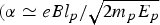 $({\rm \alpha} \simeq eBl_p /\sqrt {2m_p E_p}$). This kind of field topology induces the proton signal to exhibit an annular shape related to the azimuthal geometry of the field (as shown in Fig. 4 where arrows show the difference between the outer and inner radius of the annulus). Protons are swept out of the region corresponding to the azimuthal field, thus producing a whiter zone on the detector, and are accumulated in the outer region thus producing a darker ring on the detector. The extent of the annular pattern provides information about the field spatial distribution. It has to be noted, however, that the proton radiography does not provide a simple homothetic image of the probed field distribution. The field structure crossed by the proton beam induces a lens effect: the outer radius of the annular zone (identified by the sharp circular ring where protons pile up) is indicative of the azimuthal field extent but it is not directly proportional (by a simple magnification factor) to it. Indeed the field amplitude and the integrated path protons go through also play a role in defining the outer limit. Regions with no field are crossed by unperturbed protons: here, the laminar proton beam produces a point projection image. The internal radius of the annulus corresponds then to the edge region of the magnetic fields: it sets the limit between a region of no—or low—field, where the imaging corresponds to a point projection, and the region where the field produces a lens effect.
Fig. 4. (Color online) Two typical modulation patterns of proton radiography corresponding to (a) Gaussian intensity distribution on target (RPP) and (b) Flat top intensity distribution on target. The difference between the external radius (accumulation ring) and internal radius (start of the depletion region) is indicated. The two patterns are very similar.
The first information produced by proton radiography is then given by the shape of the modulation: we note (see Fig. 4) that PZP and RPP interactions produce similar maps even if the laser irradiation patterns are not similar. This suggests that the integrated differential trajectories of the probing particles into the field region, responsible of the modulation signal, were similar.
The second information is provided by the global extent of the modulation signal that hints at the position and the evolution of the fields. Because of the difference in size of the spots given by the two phase plates, a difference of a factor of about 2 was expected for the size (radius) of the proton modulation pattern. However, no major difference can be observed for the different plates at the same probing time: the self generated fields evolve towards a common topology. This evidence, together with the measure of a slower propagation of the heat flux for the RPP beam, suggests that the larger relative extent of the Gaussian field might be responsible of a major radial flux rotation and a consequent reduction of longitudinal flux.
In the third place, from the modulation signal we can retrieve an estimate of the B × l p product and eventually of the amplitude of the fields. As can be noticed in Figures 4 and 5, the global deflection undergone in average by those protons crossing the field region can be evaluated as the distance (indicated in Fig. 5) from the center of the whiter depletion region to the darker accumulation ring. This is roughly about 2 mm on the detector plane: for a distance D = 35 mm (interaction target-detector) this means a deflection angle α of ~50 mrad. For protons with energy E p ≃ 6 MeV the product B × l p is then of the order of 0.02 [T m]: an average B field of 100 T with a plume-like distribution extending on l p ≃ 200 µm would be needed to produce such modulation. This is in the same order of magnitude as predicted by numerical simulations, although significant difference remains between measurement and simulations concerning the position of the fields (see Section 3.2).
Fig. 5. (Color online) lineouts of measured density modulation signal and lineouts of simulated deflection pattern extracted from CHIC B fields. (a) Good agreement for a low flux. (b) High flux PZP case. Here, the measured fields expanded quicker than the simulated ones. The arrow shows the average deflection of protons: from the middle of the depletion region to the accumulation region.
We recall that, due to the nature of this diagnostic, absolute values of the B-field amplitude cannot be directly retrieved. An indirect comparison with simulated B fields can however be performed. The trajectories that protons undergo into numerically evaluated fields can be simulated; the associated proton signal on the detector can then be compared with the experimentally measured one.
Numerical investigation of this aspect will be discussed below.
3. SIMULATIONS
Numerical simulations of the laser-plasma interaction were performed using the hydrodynamic code CHIC (Maire et al., Reference Maire, Abgrall, Breil and Ovadia2007). This code is 2-D (treating longitudinal and radial directions assuming symmetry around the longitudinal axis), it accounts for two temperatures and solves the standard conservation equations for mass, momentum and energy of the fluid. It is a radiative transport code, where the propagation and absorption of the laser are calculated via three-dimensional ray-tracing. It accounts for, thermonuclear burn, macro and mesoscopic model for e − and p + transport and spreading, local and non-local thermodynamic equilibrium opacities and equation of state (QEOS and Sesame). It can be used with a flux limited Spitzer Härm heat transport package, or with a kinetic model for non-local transport which includes self-generated fields.
The mechanisms of generation and evolution of the self-generated B-fields, as described in the induction equation (Haines et al., Reference Haines1986), are modeled. Simulations were performed with a heat propagation model where the non-local features of heat transport were considered together with the Nernst velocity (Kho et al., Reference Kho and Haines1985) governing the B-fields advection. A set of simulations was performed taking into account the actual thicknesses of the layers in the target (as given by the RBS measurements), the experimental laser temporal profile and laser spot envelope shape (the hot spots within the focal spot produced by the phase plates were however neglected). Since the code relies on a cylindrical symmetry, the ellipticity of the focal spot on the target, due to the oblique incidence, could not be simulated. A circular spot with an area equal to the one of the elliptical projection of the real spots on the target was then used. This assumption was justified by the natural circular symmetrization of the flow by the plasma, as evidenced by the X-ray pinhole camera images. Finally, the laser energy in the simulations was varied in order to scan different intensities in a range comparable with the experimental conditions. The code CHIC is also equipped with different post-processors. We used such a post-processor tool to evaluate the delay in the emission of the tracers discussed above.
3.1. Postprocessing the Tracers Emission
We recall that the tracers start emitting in the X-ray domain when they are reached by the heat front propagating in the target. Detailed atomic physics of the L shell of the potassium bromide tracer could not be simulated. For this reason, two tracers of aluminum were simulated instead, the triggering emission plasma temperature being similar in the observed spectral range for brome and aluminum. There is however some incertitude on the mass heating rate which might be different for brome and aluminum and might cause the slope of the profile of the emitted signal as a function of time (i.e., the rise time) to be different. Simulations show however that the radiative switch-on of the second tracer develops more smoothly, pointing to the fact that the heat front has been bent during propagation till it has reached the second tracer. As a consequence the difference between both tracer emission rise times is less pronounced in the simulation than in the experiment. Moreover, this 2-D effect appears to be more pronounced when simulating illumination by the RPP smoothed beam. In agreement with the general trend of the measurements, the longitudinal heat flux of the Gaussian (RPP) intensity interaction is slower. A simulation taking into account just the heating of the second (deeper) tracer shows that the heating profile is not affected by the signal coming from the first.
The simulated delays are plotted in Figure 3b (full symbols). Except for the lowest intensity case, simulated delays are 15–20% smaller than the measured ones pointing to the fact that some heating inhibition mechanism, whose influence increases with the laser intensity in the range studied here, is not properly taken into account in the model. This mechanism is very likely related to the evolution of the self-generated B-fields. We stress that the general behavior of a slower heat flux associated to the Gaussian (RPP) focal spot is found in simulations, in agreement with experimental results.
3.2. Postprocessing the B fields to simulate the proton radiography
Measured proton signals were compared with the ones obtained numerically by probing the CHIC simulated fields. For doing so, the post-processing code, uses the 2D B-field maps calculated by CHIC where one dimension is set along the proton probing propagation direction and the other is radial. The B-field map has a plume-like shape that develops at the edge of the laser spot and extends outwards both radially and longitudinally for about 200 µm. The output of the post-processing is a proton density modulation on the projection plane xz. A radial density lineout can be plotted (see Figs. 5a, 5b). From a comparison with the experimental maps we can say that while the shape of the modulation pattern, as expected, confirms an azimuthal field distribution as the one calculated by the code, the experimental B-field extent (i.e., the external diameter ofthe annular shape in the proton radiography profiles), which is associated to the the region where the fields have drifted, is clearly larger than the simulated field extent. This conclusion holds for both laser illumination spots (see Figs. 6a, 6b). Moreover, simulations suggest a larger extent of the deflection pattern for Super-Gaussian (PZP) focal spots which is not found in measurements. This does not apply to shots with low flux, pointing out to some mechanism arising at high intensities. This disagreement suggests that the fields might have drifted out quicker than expected by simulations, as already reported in (Willingale et al., Reference Willingale, Thomas, Nilson, Kaluza, Bandyopadhyay, Dangor, Evans, Fernandes, Haines, Kampediris, Kingham, Minardi, Notley, Ridgers, Rosmuz, Sherlock, Tatarakis, Wei, Najmudin and Krushenick2010). This imperfect description of the fields, pointed out by the proton radiography, might also be the cause of the discrepancy between the simulated heat flux velocity and the measured one. Note that the present simulations do not take into account a source of flux inhibition that is associated with the fast drift of B-fields. Since the B-fields act by rotating the heat flux toward the radial direction, the more these fields extend the more the flux is rotated. The different behavior of RPP-produced fields, that extend over larger (relative to the spot size) zones than PZP-produced fields, confirms that more extended fields slow down the flux.
Fig. 6. (Color online) Radial distance of the proton modulation signal from the laser axis on the target plane, as a function of laser intensity, as extracted from (a) measurements and (b) simulations for both phase plates. Fields have traveled further than predicted by simulations. The bars represent the difference between the outer and the inner radius of the modulation region as shown in Figure 4. The low flux shot is not included since it was probed at a later time.
4. DISCUSSION
Our experiment shows that B-fields associated to a 100 µm Gaussian intensity distribution extend over a larger region (relatively to the laser spot size) and slow down the longitudinal heat flux compared to a 200 µm flat top laser intensity distribution. Proton radiography of these B-fields confirms previous results stating that B-fields evolve faster than expected by numerical models (Willingale et al., Reference Willingale, Thomas, Nilson, Kaluza, Bandyopadhyay, Dangor, Evans, Fernandes, Haines, Kampediris, Kingham, Minardi, Notley, Ridgers, Rosmuz, Sherlock, Tatarakis, Wei, Najmudin and Krushenick2010). This strongly suggests that both fast advection of B-field and stronger heat flux inhibition are related to each other. Since both the size and the shape of the focal spot we used were different, it is not clear which of these parameters is more involved in being responsible for our observations. However we recall that CHIC simulations agreed almost perfectly with the measured heat transport velocity during the experiment reported in Schurtz et al. (Reference Schurtz, Gary, Hulin, Chenais-Popovics, Gauthier, Thais, Breil, Durut, Feugeas, Maire, Nicolai, Peyrussse, Reverdin, Soullié, Tikhonchuk, Villette and Fourment2007), despite the higher intensity reached in that experiment. During this experiment, the focal spot was Gaussian shaped with a 380 µm FWHM and the longitudinal spectral dispersion smoothed the hot spots generated by the phase plate. This suggests that the size of the laser spot is of prime importance, even if hot spots can also be thought to play an important role. Finally, it is clear that the treatment of the evolution of self-generated B-fields needs to be revisited to accurately model heat transport in the conditions of our study.
ACKNOWLEDGMENTS
The authors would like to acknowledge V. Tickonchuck, P. Audebert and O. Peyrusse for valuable discussion, the helpful support of LULI teams, Marc Faucon from ALPHANOV (target machining/cutting) and CENBG (target characterization with RBS).

