The study of corruption—its causes, effects, and persistence—is a matter of great interest to both the scholarly and policy communities. Corruption is recognized as a threat to economic development, democratic consolidation, and human dignity. Consequently, the desire to reduce corruption has become an important goal of international financial institutions, civil society groups, and individual nations’ domestic and foreign policies.
Two stylized facts related to corruption have been influential in how academics, policymakers, and others think about whether and how it is possible to attain these goals. First, the prevalence of corruption varies significantly across different contexts. This variation can be seen cross-nationally (e.g., Treisman Reference Treisman2007), as well as within countries; for example, there are large differences in corruption across American states (Alt and Lassen Reference Alt and Lassen2003; Glaeser and Saks Reference Glaeser and Saks2006) and cities (Menes Reference Menes2006); between Southern and Northern Italy (e.g., Banfield and Banfield Reference Banfield and Banfield1958; Golden and Picci Reference Golden and Picci2005); and across states in India (Transparency International India 2005). Such variation gives reformers hope that corruption can indeed be reduced, that “high-corruption” countries or regions can be turned into “low-corruption” countries or regions.
However, it is also the case that high or low levels of corruption tend to be very persistent: we rarely observe high-corruption countries or regions becoming low-corruption countries or regions, or vice versa (see Figure A1 in the Supplemental Appendix; see also Damania, Fredriksson and Mani Reference Damania, Fredriksson and Mani2004; Becker et al. Reference Becker, Boeckh, Hainz and Woessmann2016).Footnote 1 One plausible explanation for this persistence in corruption levels is that the dynamics underlying corruption allow for multiple equilibria. The existence of multiple equilibria can lead to differences among similar countries and regions driven by whether they play the “low-corruption” or “high-corruption” equilibrium; if countries or regions consistently play the same equilibrium, these differences will persist over time.
This explanation has received significant theoretical attention. Most of the previous accounts focus on interactions between a fixed set of bureaucrats or politicians, proposing that incentives to engage in corrupt behavior may increase as government officials come to believe that other government officials are also corrupt. These mutually reinforcing beliefs create strategic complementarities which can then lead to multiple equilibria: a low-corruption equilibrium where bureaucrats or politicians refrain from corruption when they believe that others will do so, and a high-corruption equilibrium where they engage in corruption in the belief that others will be corrupt as well. For example, in Cadot (Reference Cadot1987), the high prevalence of corruption implies that higher-level bureaucrats are more tolerant of lower-level corruption. In Mishra (Reference Mishra2005), the cost of compliance increases as others become increasingly non-compliant, lowering the benefits from being “clean” (see also Mauro Reference Mauro2004). In Andvig and Moene (Reference Andvig and Moene1990), the high incidence of corruption lowers the search costs of the briber for a willing bribee, and lowers the probability of detection from engaging in corruption (see also Lui Reference Lui1986).Footnote 2
We build on this approach based on strategic complementarities, but highlight two important shortcomings of the existing literature. First, we argue that to describe the politics of multiple equilibria of corruption more fully, it is important to focus not just on a fixed set of politicians or bureaucrats, but also on voters and potential candidates for political office (“entrants”), as well as the interactions among these three sets of actors. In principle, bureaucrats are accountable to politicians, who in democracies are accountable to voters.Footnote 3 This electoral accountability should in principle make it easier to escape the high-corruption equilibrium.
However, empirical research on voters’ reactions to corruption shows that not all electorates unconditionally punish corruption. Klašnja and Tucker (Reference Klašnja and Tucker2013) conduct a survey experiment examining voters’ reactions to economic performance and corruption in a low-corruption country (Sweden) and a high-corruption country (Moldova). They find that in Sweden voters react negatively to corruption regardless of the state of the economy, whereas in Moldova voters react negatively to corruption only when the state of the economy is also poor. Elsewhere, scholars have similarly found that in higher-corruption countries, voters are often insensitive to corruption (Banerjee and Pande Reference Banerjee and Pande2009; Manzetti and Wilson Reference Manzetti and Wilson2007; Zechmeister and Zizumbo-Colunga Reference Zechmeister and Zizumbo-Colunga2013; Klašnja, Tucker and Deegan-Krause Reference Klašnja, Tucker and Deegan-Krause2016), sometimes even when given precise information about it.Footnote 4 Voters in low-corruption countries tend to punish corruption more consistently (Welch and Hibbing Reference Welch and Hibbing1997; Reed Reference Reed1999; Hirano and Snyder Reference Hirano and Snyder2012).Footnote 5 This suggests that voters’ behavior may contribute to the multiplicity of equilibria in corruption prevalence.
A second shortcoming of much of the existing literature is that high-corruption equilibria driven mainly by expectations of how corrupt others will be suggest a particular anti-corruption policy prescription: an intervention that rapidly changes the corruption expectations of a fixed set of actors. While such interventions are not costless, they seem feasible, and yet, they appear inconsistent with the fact that corruption persists across countries and regions. Instead, we argue that high-corruption equilibria may be hard to escape because they are driven by the prevalence of particular types of politicians, both those in office and those willing to enter politics, as well as the interaction among politicians and with voters. Our models thus exhibit more of the strategic complementarities that lead to multiple equilibria than past models suggest, highlighting why acting on bureaucrats’ expectations alone may not be enough to reduce corrupt behavior.Footnote 6
Our analysis builds on a simple model of corrupt behavior among politicians in office. Politicians vary based on their predisposition to engage in corrupt behavior (as well as ability), and choose a level of corrupt activity where the benefits from doing so are a function of the degree to which other politicians choose to engage in similarly corrupt behavior. This analysis has two important properties that drive our results about voter (and entrant) behavior. First, a given politician engages in more corrupt behavior when others in office are more predisposed to corruption. Second, the relative value of holding office for a politician is higher for those predisposed to corruption, and, in line with the above-mentioned work on multiple equilibria of corruption, the size of this “politician corruption differential” is increasing in the level of corruption. When combined with our assumptions about citizen preferences, the second point implies that as politics becomes more corrupt, citizens can become more tolerant of corrupt politicians, and thus less apt to vote them out of office.
We then proceed to show how these results affect the behavior of voters and potential candidates. In our main model, voters observe the ability and corruption predisposition of their current representative and decide whether to keep or replace her. If voters become more tolerant or even prefer corrupt representatives as others are more corrupt, there can be multiple equilibria: one equilibrium where voters are generally willing to retain corrupt politicians, and one where voters generally replace corrupt politicians. We call the former situation a “political corruption trap.” Next, we draw on Caselli and Morelli (Reference Caselli and Morelli2004) in deriving a model that examines a similar complementarity between potential entrants, where those predisposed to corruption are more apt to run when they expect others to be corrupt as well. Importantly, we also show that when the dynamics from the voter and politician models are combined with the dynamics of the entry model, the potential for a political corruption trap is generally even greater.
Our analysis is related to but differs from several other important previous contributions that have also investigated the roles of political incentives and heterogeneity in politician types in persistence of corruption or quality of accountability more broadly. The closest model to our analysis of entry decisions is the model by Caselli and Morelli (Reference Caselli and Morelli2004), who argue that the current share of “bad” politicians will affect the relative returns to office-holding for other bad politicians. Our paper builds on this argument by primarily focusing on the strategic complementarities in voters’ tolerance of corruption, while also exploring the interaction between voters’ selection decisions and candidate entry dynamics.Footnote 7
The possibility of multiple accountability equilibria arising from the interaction between voters and politicians has also been explored in recent related papers by Ashworth, Bueno de Mesquita and Friedenberg (Reference Ashworth, Bueno de Mesquita and Friedenbergforthcoming) and Svolik (Reference Svolik2013). Both papers describe a trap due to voters’ pessimistic expectations: a bad equilibrium where politicians exert little effort when little is expected of them. While we echo this result in our analysis as well, we focus more closely on how daunting this task of changing expectations may be if the goal is to bring about a reduction in corruption.Footnote 8
This paper proceeds as follows. The second section lays out our main model of politician and voter behavior, which in turn can lead to a corruption trap. These corruption traps depend on a particular configuration of politician types; however, in the third section we describe traps arising from proportions of corrupt politicians that would be stable over time, independent of the particular distribution of politician types in any given election. The penultimate section briefly discusses our model of the behavior of entrants and corruption traps that arise therein, and more importantly, how corruption traps can arise through interactions between politicians, voters, and entrants. The last section summarizes our results and discusses their implications and directions for future research.
The Model
Consider a country with N geographic units (e.g., cities, counties, or legislative districts). Each unit contains a voter (V), an incumbent politician (I), and a challenger (C). This environment could correspond to an electoral system where legislators are elected by plurality vote in single-member constituencies. In a proportional representation system (and elsewhere), the model could also describe the choice of directly elected local executives, such as governors or mayors.Footnote 9
Politicians are characterized by a two-dimensional type which captures their general ability and predisposition to corruption. Let
 $a_{i}^{I} $
and
$a_{i}^{I} $
and
 $c_{i}^{I} $
be the ability and corruption predisposition for the incumbent politician in district i. The challenger’s ability and predisposition are
$c_{i}^{I} $
be the ability and corruption predisposition for the incumbent politician in district i. The challenger’s ability and predisposition are
 $a_{i}^{C} $
and
$a_{i}^{C} $
and
 $c_{i}^{C} $
. We assume that
$c_{i}^{C} $
. We assume that
 $$a_{i}^{J} \,\geq \,\underline{a} \,\,\gt\,\,0$$
(J∈{I, C}), where
$$a_{i}^{J} \,\geq \,\underline{a} \,\,\gt\,\,0$$
(J∈{I, C}), where
 $\underline{a} $
is the “minimum” ability level. The predisposition for corruption is binary, where
$\underline{a} $
is the “minimum” ability level. The predisposition for corruption is binary, where
 $c_{i}^{J} \,{\equals}\,0$
indicates no predisposition toward corruption (“clean”), while those with
$c_{i}^{J} \,{\equals}\,0$
indicates no predisposition toward corruption (“clean”), while those with
 $c_{i}^{J} \,{\equals}\,1$
have a predisposition toward corruption.
$c_{i}^{J} \,{\equals}\,1$
have a predisposition toward corruption.
The voters decide which candidate to elect, and then the elected politicians decide how to allocate their time between corrupt and non-corrupt activities. The voter knows the type of the incumbent but not the challenger.Footnote 10 Let F be the cumulative distribution function for the challenger ability, and q∈(0, 1) the probability that a challenger is corrupt. We assume that F is continuous and differentiable, and that a politician’s predisposition to corruption and ability are independent. Once elected, the politician types become common knowledge. When referring to the elected politician, we drop the superscripts, so the type of the elected politician in district i is (a i , c i ).
Politicians have an amount of effort to exert equal to their ability. Effort can be spent on corrupt activities x i ≥0 and other non-corrupt activities y i ≥0. Formally, politicians choose x i and y i subject to a “budget constraint” x i +y i ≤a i . Let the utility for the elected politician (u P ) and voter (u V ) in district i be
 $$u^{P} \,(x_{i} ,\,y_{i} ;c_{i} )\,{\equals}\,y_{i} {\plus}c_{i} g(x_{i} ,\,\bar{x}),$$
 $$u^{V} \,(x_{i} ,\,y_{i} )\,{\equals}\,y_{i} {\plus}bg(x_{i} ,\,\bar{x}).$$
(The non-elected politicians take no actions, and so their preferences do not affect the analysis.)
The first term of both utilities captures the returns to non-corrupt activity. For simplicity we set this equal to the effort allocated for both politician and voter. Importantly, we assume that the returns to non-corrupt activity do not have externalities for the politicians in other districts, as we will do for corrupt activities.Footnote 11
Politicians with c
i
=0 get no benefit from corrupt behavior.Footnote
12
Those who are predisposed toward engaging in corrupt behavior get a partial payoff that is a function of their corruption choice (x
i
) and the average level of corruption chosen by others
 $(\bar{x})$
, captured by
$(\bar{x})$
, captured by
 $g(x_{i} ,\,\bar{x})$
term. We assume that g is continuous and twice differentiable, with
$g(x_{i} ,\,\bar{x})$
term. We assume that g is continuous and twice differentiable, with
 $g(0,\bar{x})\,{\equals}\,0$
, meaning that there is no return to corruption if the politician allocates no effort to this end.
$g(0,\bar{x})\,{\equals}\,0$
, meaning that there is no return to corruption if the politician allocates no effort to this end.
To express the remaining assumptions on g, we use the common notation where g 1 is the partial derivative of g with respect to its first argument (in this case x i ), g 2 the partial derivative of g with respect to the second argument, g 11 the second derivative with respect to the first argument, g 12 the cross-partial derivative, etc. In particular, let the returns to corruption be increasing (g 1>0) and concave (g 11<0) in the effort allocated; that is, there are diminishing marginal returns to corrupt behavior. In line with the literature on strategic complementarities in corrupt behavior we reviewed above, we assume that the return to corruption and the marginal return to more corrupt behavior are both increasing in how corrupt other politicians are (g 2>0 and g 12≥0).Footnote 13
Now consider how corrupt behavior affects the voter (or, more precisely, the pivotal voter). For negative b, the citizen’s payoff is decreasing in the corruption payoff earned by the politician. Voters may be directly harmed by the corrupt behavior of their representatives (in addition to the foregone effort the representatives could have made toward more productive ends) for a myriad of reasons, including negative effects of corruption on outcomes like investment (Mauro Reference Mauro1995) and human capital accumulation (Reinikka and Svensson Reference Reinikka and Svensson2004). However, even if corruption generally harms the pivotal voter, she may sometimes benefit when her representative is corrupt, implying b>0. While b≥1 is unlikely (i.e., that the voter benefits above and beyond the politician’s own corrupt payoff; we do not consider this case hereafter), b∈(0,1) implies that the voter’s payoff is increasing in the corruption payoff earned by the politician, but scaled downward. There are numerous examples of re-election-seeking politicians funneling some of the corrupt rents to their electorate or political parties through vote-buying campaigns and patronage. For example, coronéis, local political bosses in Brazil, have long used corrupt revenues to broker votes (Mainwaring Reference Mainwaring1999; Gingerich Reference Gingerich2014). We provide additional examples and further discussion of this assumption in Section A2 in the Supplemental Appendix.
The following timeline summarizes the sequence of moves:
We first solve for the perfect Bayesian equilibria (PBE) of the model, and then search for a proportion of corrupt politicians that is stable in the long term.
Politician Stage
The politician strategies are a function mapping their corruption level and ability to an allocation of effort (x i , y i ), where these strategies must be mutual best responses.
As politicians with c i =0 get no benefit from corruption, they allocate all of their effort to non-corrupt activities. Since the payoff for a corrupt politician is increasing in both x i and y i , they always use the entire effort budget: x i +y i =a i . So, corrupt politicians choose an x i that maximizes
 $$u^{P} \,(x_{i} ,\,a_{i} {\minus}x_{i} ; c_{i} )\,{\equals}\,a_{i} {\minus}x_{i} {\plus}g(x_{i} ,\,\bar{x}).$$
Let ρ=∑ i (c i −1)/(N−1) be the proportion of the other politicians that are predisposed to corruption from the perspective of one who is corrupt. The equilibrium condition for a symmetric interior x* is then given by
 $$g_{1} (x^{{\asterisk}} ,\,\rho x^{{\asterisk}} )\,{\equals}\,1.$$
The marginal benefit to allocating an additional unit of effort to non-corrupt activities is always 1, so this condition states that corrupt politicians get the same marginal benefit from allocating more effort to corruption, given the fact that other corrupt politicians also choose x*. Under mild restrictions, there is a unique interior solution in the politician stage, where corrupt politicians allocate more of their time to illicit activities when many others are corrupt:
Proposition 1
Given the assumptions on g stated above and (1) g
11(x, ρx)<−ρg
12(x, ρx), (2) g
1(0, 0)>1, and (3)
 $g_{1} (\underline{a} ,\,\rho \underline{a} )\,\lt\,1$
, the politician stage has a unique interior equilibrium level of corruption x* chosen by politicians with c
i
=1 characterized by Equation 1. In equilibrium:
$g_{1} (\underline{a} ,\,\rho \underline{a} )\,\lt\,1$
, the politician stage has a unique interior equilibrium level of corruption x* chosen by politicians with c
i
=1 characterized by Equation 1. In equilibrium:
i. the level of corrupt activity for those predisposed to corruption is increasing in ρ, and
ii. the relative payoff of a corrupt politician (u P (c i =1; x*)−u P (c i =0; x*)) is positive and increasing in ρ.
All proofs can be found in the Supplemental Appendix.
Condition (1) implies that the diminishing returns effect of higher corruption levels (g 11(x, ρx)) is stronger (i.e., more negative) than the strategic complementarity effect (−ρg 12(x, ρx)). If this does not hold, there may be multiple equilibria in the politician stage by the standard logic of corruption traps in the existing literature presented above. To bring attention to a mechanism through which high- and low-corruption equilibria emerge for other reasons, we assume this does not occur.
Conditions (2)–(3) prevent a corner solution where some corrupt politicians either allocate all or none of their effort to corrupt behavior, which reduces the number of cases to consider. Therefore, conditions (1)–(3) imply a unique interior corruption level. Because of the strategic complementarities, adding more corrupt politicians makes those predisposed to corruption allocate even more effort to corruption. Further, since g 2>0 (and by the envelope theorem), office-holding becomes more valuable for corrupt politicians as ρ increases, a convenient fact when considering endogenous entry.
Voter Stage
Now consider voters’ decisions given politician behavior. A voter with a non-corrupt politician who allocates all of her effort to other activities attains utility a i . A voter with a corrupt politician who allocates x* to corrupt activities and a i −x* to other activities attains a i −x*+bg(x*, ρx*). Define the voter corruption differential as the utility difference between having a corrupt versus non-corrupt politician:
 $$d^{V} \,(\rho ,\,x^{{\asterisk}} )\,{\equals}\,a_{i} {\minus}x^{{\asterisk}} {\plus}bg(x^{{\asterisk}} ,\,\rho x^{{\asterisk}} ){\minus}a_{i} \,{\equals}\,bg(x^{{\asterisk}} ,\,\rho x^{{\asterisk}} ){\minus}x^{{\asterisk}} .$$
Conveniently, this is not a function of a i : voters always prefer more able politicians, but the ability does not affect the relative value of having a corrupt or clean representative.
The expected payoff to choosing a challenger is then
 ${\Bbb E}[a]{\plus}qd^{V} (\rho ,\,x^{{\asterisk}} )$
, and so for a fixed ρ the voter prefers a replacement to an incumbent politician with
${\Bbb E}[a]{\plus}qd^{V} (\rho ,\,x^{{\asterisk}} )$
, and so for a fixed ρ the voter prefers a replacement to an incumbent politician with
 $(a_{i}^{I} ,\,c_{i}^{I} )$
if
$(a_{i}^{I} ,\,c_{i}^{I} )$
if
 $$a_{i}^{I} \,\leq\, {\Bbb E}[a]{\plus}(q{\minus}c_{i}^{I} )d^{V} \,(\rho ,\,x^{{\asterisk}} ).$$
The voter’s decision is always monotone in the ability of their politician, but the threshold in ability will be different for a corrupt and a non-corrupt politician. If voters in other districts become more or less tolerant of corruption, this can change the calculus of a voter through changing expectations about ρ.
Most relevant for characterizing the equilibrium is determining the shape of the d V (ρ, x*) function. It will be particularly important to know when the voter corruption differential can be increasing in ρ, which will broadly imply strategic complementarities among voters in the degree to which they tolerate corruption. More precisely, where d V (ρ, x*) is positive (i.e., the voter’s utility from a corrupt politician is higher than from a clean politician), d V (ρ, x*) increasing in ρ implies that voters prefer a corrupt politician and that the magnitude of this preference is increasing in the general prevalence of corruption. It is also possible that d V (ρ, x*) is negative but increasing in ρ, which means that voters prefer a clean politician but become relatively more tolerant of corruption as it becomes more prevalent. In either case, the total derivative of the voter corruption differential (accounting for the effect on x*) is
 $${d \over {d\rho }}\left[ {d^{V} \,(\rho ,\,x^{{\asterisk}} )} \right]\,{\equals}\,{\minus}{{\partial x^{{\asterisk}} } \over {\partial \rho }}{\plus}b{d \over {d\rho }}\left[ {g(x^{{\asterisk}} ,\,\rho x^{{\asterisk}} )} \right].$$
Since the emphasis in characterizing the voter behavior will be on how their decisions affect ρ, for the remainder of the paper we suppress the x* argument in the voter corruption differential, writing it d V (ρ). Thus, when we say this function is increasing (decreasing), we mean that as more (fewer) politicians are corrupt, the relative value of having a corrupt representative increases (decreases), accounting for the change in x*.
There are two competing effects on the voter corruption differential as the prevalence of corruption increases. First, corrupt representatives allocate less effort to non-corrupt activities (the
 ${\minus}{{\partial x^{{\asterisk}} } \over {\partial \rho }}$
term), reducing the relative value to the voter of having a corrupt politician. However, the returns to corruption increase, and if citizens enjoy some of the fruits of corruption, they can benefit from this as well. Whether more corrupt politics makes having a corrupt representative more or less valuable for the voter depends on which of these two effects dominates.
${\minus}{{\partial x^{{\asterisk}} } \over {\partial \rho }}$
term), reducing the relative value to the voter of having a corrupt politician. However, the returns to corruption increase, and if citizens enjoy some of the fruits of corruption, they can benefit from this as well. Whether more corrupt politics makes having a corrupt representative more or less valuable for the voter depends on which of these two effects dominates.
When b≤0, citizens get no benefit from corruption, and so the only effect of increasing ρ is that corrupt politicians allocate less effort to non-corrupt activities, which hurts their constituents. As a result, the voter corruption differential is decreasing. On the other hand, if b=1, the citizens payoff from corruption is exactly the same as their politician’s, and part (ii) of Proposition 1 is equivalent to stating that d V (ρ) is increasing. In between these extremes, the relative value of having a corrupt representative is increasing in ρ if and only if citizens get a high enough benefit from corrupt activity:
Proposition 2
If
 $b\,\gt\,\tilde{b}$
for some
$b\,\gt\,\tilde{b}$
for some
 $\tilde{b}\in(0,\,1)$
, the voter corruption differential is increasing in ρ.
$\tilde{b}\in(0,\,1)$
, the voter corruption differential is increasing in ρ.
The intuition behind Proposition 2 is that even if citizens only get a small benefit from their representatives’ corrupt behavior, they may prefer this fraction of the proceeds to having a completely clean politician in a highly corrupt environment.Footnote 14
When can this complementarity lead to multiple equilibria? As long as at least one voter replaces their politician, all the voters become uncertain about the number of corrupt politicians who will end up in office. So, the details of which politicians are retained in equilibrium depend on the distribution of ability among the corrupt and non-corrupt politicians. Still, a standard existence argument ensures that there will be some (potentially mixed strategy) PBE to the model. Rather than present all of the cases here, we highlight two sufficient conditions under which there are multiple equilibria with different levels of tolerance of corruption:
Proposition 3 The model has at least one PBE. Further:
i. if d V (ρ) is locally increasing between two feasible corruption levels (formally, if there exists an integer n′ such that d V (n′/(N−1))>d V ((n′−1)/(N−1)), then for some distributions of incumbent types the model has multiple equilibria where a different number of corrupt politicians are replaced, andFootnote 15
ii. if d V (ρ) is increasing for all ρ, then for any number of corrupt incumbents there exist distributions of incumbent types that result in multiple equilibria where either all of the corrupt politicians are kept or all are replaced.
The intuition behind part (i) is that if d V (ρ) is increasing locally around a particular corruption level, then if one other constituency were to remove their corrupt politician, a voter who was previously slightly in favor of keeping their own corrupt incumbent would vote him out as well. So, if there are two politicians who are just above the threshold for retention, then there is one equilibrium where both are retained, and one where both are replaced. Part (ii) follows a similar logic: if voters are always more tolerant of corruption when others are corrupt, and all of the corrupt politicians are just above the ability threshold where the voter keeps them if every other voter with a corrupt politician does so, then there is one equilibrium where all of the corrupt politicians are retained and one where they are all removed from office.Footnote 16
Even if an increasing voter corruption differential is plausible, the logic behind Proposition 3 requires a very particular configuration of politician types, which may not always be likely. To search for more robust results, we now consider the corruption traps arising from conditions in which the proportion of corrupt politicians are stable over time, independent of the particular distribution of ability at any given election.
Long-Run Stable Prevalence of Corruption
We formalize the notion that the proportion of corrupt politicians is stable as follows:
Definition A long-run equilibrium to the voter model comprises a symmetric corruption choice x* and ability thresholds
 $$\hat{a}_{0} $$
and
$$\hat{a}_{0} $$
and
 $$\hat{a}_{1} $$
that jointly solve
$$\hat{a}_{1} $$
that jointly solve
 $$x^{{\asterisk}} \,{\equals}\,{\rm arg}\,\mathop {{\rm max}}\limits_x \,a_{i} {\minus}x{\plus}g(x,\,\rho \bar{x}),$$
 $$\hat{a}_{1} \,{\equals}\,{\Bbb E}[a]{\minus}(1{\minus}q)d^{V} \,(\rho ),$$
 $$\hat{a}_{0} \,{\equals}\,{\Bbb E}[a]{\plus}qd^{V} \,(\rho ),$$
 $$\rho \,{\equals}\,{{q(1{\minus}F(\hat{a}_{1} ))} \over {q(1{\minus}F(\hat{a}_{1} )){\plus}(1{\minus}q)(1{\minus}F(\hat{a}_{0} ))}}.$$
Equations 2–4 are just the equilibrium conditions from the model in the previous section when there is a fixed and known proportion of corrupt politicians. Equation 5 implies that the proportion of corrupt politicians is equal to the conditional probability of being corrupt for politicians who are able enough to be retained (given their predisposition to corruption).
Finding an equilibrium can be reduced to finding a fixed point ρ* which allows for a joint solution to 2–5. To find this fixed point, first define the probability of a randomly drawn politician having a high enough ability to be kept if clean
 $(q_{0}^{k} )$
and corrupt
$(q_{0}^{k} )$
and corrupt
 $(q_{1}^{k} )$
as
$(q_{1}^{k} )$
as
 $$\eqalignno{ & q_{0}^{k} (\rho )\,{\equals}\,(1{\minus}q)(1{\minus}F({\Bbb E}[a]{\plus}qd^{V} \,(\rho ))), \cr & q_{1}^{k} (\rho )\,{\equals}\,q(1{\minus}F({\Bbb E}[a]{\minus}(1{\minus}q)d^{V} \,(\rho ))). $$
We can then collapse the equilibrium condition to finding a ρ which solves
 $$\rho {\equals}{{q_{1}^{k} (\rho )} \over {q_{0}^{k} (\rho ){\plus}q_{1}^{k} (\rho )}}\,\equiv\,\bar{q}(\rho ).$$
The
 $\bar{q}(\rho )$
function, which captures the relative likelihood of a politician being corrupt given she is good enough to be kept, is continuous and bounded by (0, 1), and so there must be at least one ρ*∈(0, 1) that satisfies Equation 6. To determine whether the intersection (and hence the stable level of corruption) is unique, differentiating the right-hand side with respect to ρ (and substituting the derivatives of the
$\bar{q}(\rho )$
function, which captures the relative likelihood of a politician being corrupt given she is good enough to be kept, is continuous and bounded by (0, 1), and so there must be at least one ρ*∈(0, 1) that satisfies Equation 6. To determine whether the intersection (and hence the stable level of corruption) is unique, differentiating the right-hand side with respect to ρ (and substituting the derivatives of the
 $q_{i}^{k} (\rho )$
terms) gives
$q_{i}^{k} (\rho )$
terms) gives
 $${{\partial \bar{q}} \over {\partial \rho }}{\equals}{d \over {d\rho }}\left[ {d^{V} \,(\rho )} \right]{{q(1{\minus}q)(q_{0}^{k} (\rho )f({\Bbb E}[a]{\minus}(1{\minus}q)d^{V} \,(\rho )){\plus}q_{1}^{k} (\rho )f({\Bbb E}[a]{\plus}qd^{V} (\rho )))} \over {(q_{0}^{k} (\rho ){\plus}q_{1}^{k} (\rho ))^{2} }}.$$
All terms other than the derivative of d
V
(ρ) are positive, so the sign of this expression is the same as the sign of
 $${d \over {d\rho }}\left[ {d^{V} \,(\rho )} \right]$$
. If d
V
(ρ) is decreasing, which as before implies that when more politicians are corrupt, the voter becomes worse-off with a corrupt representative, then
$${d \over {d\rho }}\left[ {d^{V} \,(\rho )} \right]$$
. If d
V
(ρ) is decreasing, which as before implies that when more politicians are corrupt, the voter becomes worse-off with a corrupt representative, then
 ${{\partial \bar{q}} \over {\partial \rho }}$
is negative, implying that Equation 6 must have a unique solution. However, if d
V
(ρ) is increasing and with a high enough slope, indicating that the relative benefit of having a corrupt politician increases quickly as the prevalence of corruption rises, then the slope of this equation can be greater than 1, raising the possibility of multiple intersections and hence multiple equilibria, one with a relatively low share of corrupt politicians and one with a relatively high share of corrupt politicians:
${{\partial \bar{q}} \over {\partial \rho }}$
is negative, implying that Equation 6 must have a unique solution. However, if d
V
(ρ) is increasing and with a high enough slope, indicating that the relative benefit of having a corrupt politician increases quickly as the prevalence of corruption rises, then the slope of this equation can be greater than 1, raising the possibility of multiple intersections and hence multiple equilibria, one with a relatively low share of corrupt politicians and one with a relatively high share of corrupt politicians:
Proposition 4
There is at least one long-run stable equilibrium to the voter model, and if
 ${d \over {d\rho }}\left[ {d^{V} \,(\rho )} \right]\leq 0$
, the equilibrium is unique. If
${d \over {d\rho }}\left[ {d^{V} \,(\rho )} \right]\leq 0$
, the equilibrium is unique. If
 ${d \over {d\rho }}\left[ {d^{V} \,(\rho )} \right]\,\gt\,0$
there may be multiple equilibria to the voter model.
${d \over {d\rho }}\left[ {d^{V} \,(\rho )} \right]\,\gt\,0$
there may be multiple equilibria to the voter model.
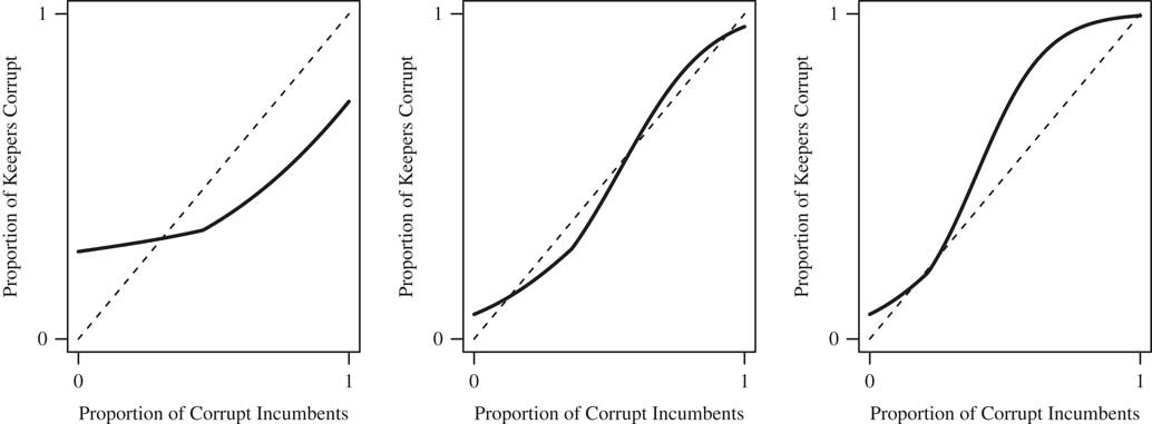
Figure 1 illustrates this result. In each panel, the solid curve is the right-hand side of Equation 6, and the dashed line is the left-hand side (i.e., the 45° line). Therefore, an intersection corresponds to a stable level of corruption. In the left panel, d V (ρ) is decreasing (i.e., having a corrupt politician makes the voter worse-off as corruption becomes more prevalent), and as a result there is a unique stable proportion of corrupt politicians. In the middle panel d V (ρ) is increasing, but at a slow rate, and so there is still a unique intersection and hence only one stable corruption level. In the right panel, d V (ρ) is increasing more sharply, and as a result there are two stable corruption levels, one where nearly all politicians are clean, and one where nearly all politicians are corrupt.
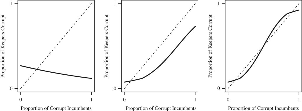
Fig. 1 Examples with one (left and middle panels) and multiple (right panel) long-run stable corruption levels Note: In all three panels, q=1/2 and ability follows an exponential distribution with rate parameter λ=1. The panels vary in d V (ρ), which is decreasing in the right panel (d V (ρ)=−1−ρ), increasing but at a relatively slow rate in the middle panel (d V (ρ)=−3+4ρ), and increasing at a faster rate in the right panel (d V (ρ)=−3+6ρ).
In sum, the possibility of multiple equilibria in the voter model provides an explanation of corruption traps that is inherently political. When there are equilibria with both a low and high level of corruption and the higher corruption equilibrium is played, the accountability mechanism does not necessarily solve problems of corruption and can perpetuate political corruption traps: voters are either tolerant of corrupt politicians or avoid clean politicians under the mutual expectation that voters in other districts will do the same. That is, the accountability mechanism requires that citizens are willing to take costly actions to remove “bad” politicians from office. In the case of corruption, if voters in district i are unwilling to vote corrupt politicians out of office, voters in district j may not be willing to do so either, if in a generally corrupt system the corrupt politicians are regarded as more effective. We discuss several examples in Section A2 of the Supplemental Appendix.
Voter Behavior with Endogenous Entry
Similar dynamics can lead to multiplicity of equilibria due to strategic complementarities among potential entrants to the political arena. Section A4 of the Supplemental Appendix contains a model where in each district a number of potential entrants decide whether or not to run for office, with the expectation that the winners will play the politician stage described above (i.e., there are no voters). Since the general logic of this model is close to our main model (and the results are of a similar flavor as those in Caselli and Morelli Reference Caselli and Morelli2004), here we only briefly describe the results from this model and their implications for our main model.
The two key results from endogenizing entry decisions are as follows: (1) the proportion of entrants who are predisposed to corruption is increasing in the expectation of how many others will be corrupt, and (2) this complementarity can lead to a multiplicity of equilibria for similar reasons as in our main model. Therefore, corruption traps can arise individually at the level of incumbents, voters, and entrants.
However, we want to stress here how even if the complementarities in the politician, voter, and entry stages do not separately lead to a political corruption trap, the interaction between the three can lead to multiple equilibria and hence a corruption trap.
To show this, we now let the proportion of entrants that are corrupt be a function of ρ, that is, q(ρ). As is predicted in Proposition A1 in the Supplemental Appendix, we assume that q is increasing, implying that more potential entrants are corrupt when more incumbents are corrupt.
The equilibrium condition is the same as before, with q(ρ) replacing the constant ρ. Figure 2 shows how the examples from Figure 1 change when there is endogenous entry. As in Figure 1, in the left panel d V (ρ) is negative, meaning that voters are more apt to punish corruption when it is more prevalent. However, unlike in Figure 1, now the proportion of retained corrupt politicians is increasing in ρ because of the increase in corrupt candidates in the pool of entrants. Nonetheless, these complementarities between politicians and entrants are not strong enough to induce multiplicity, and so there is still only one stable—and relatively low—corruption level. In the middle panel (which previously had one stable corruption level despite strategic complementarities among both politicians and voters), the combination of strategic complementarities of all three actors is sufficient to generate a corruption trap. In the right panel, as before, there are multiple stable corruption levels, but the proportion of corrupt incumbents who are retained in the high-corruption equilibrium is even higher than in Figure 1.

Summary and Discussion
The overarching conclusion of the formal models we have presented is that decisions made by incumbent politicians, potential entrants to politics, and voters all interact in a way that can lead to political corruption traps, that is, the presence of a high-corruption as well as a low-corruption equilibrium.
Figure 3 summarizes these interactions. For each of the three levels, we can think of the actors in question interdependently behaving in a way that may lead to more corruption: (1) politicians choosing to engage in more corrupt behavior, (2) voters being more tolerant of or even approving of corrupt politicians, and (3) those predisposed to corruption being more apt to enter politics. Solid arrows indicate relationships which we have formalized in the previous sections or the Supplemental Appendix. The dashed arrows represent the relationships we informally discuss below.
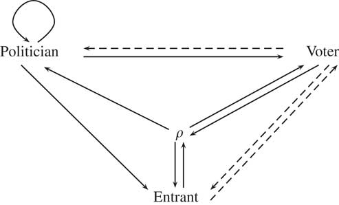
Fig. 3 Relationships between the three levels of analysis Note: ρ is the proportion of politicians predisposed toward corruption. Solid arrows indicate relationships which we have formalized in the previous sections or the Supplemental Appendix. The dashed arrows represent the relationships we informally discuss in the text.
In our models, these three levels primarily interact through the proportion of politicians predisposed toward corruption (ρ). As ρ increases, politicians choose a higher level of corruption (Proposition 1; solid arrow from ρ to politician), voters can be more tolerant of corruption (Equation 7; solid arrow from ρ to voter), and corrupt candidates are relatively more likely to enter than clean entrants (Proposition A1 in the Supplemental Appendix; solid arrow from ρ to entrant). The solid arrows from entrant/voter to ρ follow from the definition of ρ in these models: more corrupt entrants and greater voter tolerance of corruption directly lead to more corrupt politicians.
The solid arrows from politician to entrant and politician to voter indicate that even for a fixed proportion of incumbents predisposed to corruption, more corrupt behavior (i.e., greater x*) encourages corrupt entrants and induces greater voter lenience toward corruption. Finally, the insights from the Voter Behavior with Endogenous Entry section show the combined effect of ρ on the behavior of entrants and voters (combining solid arrows from ρ to voter and entrant).Footnote 17
There are other potential sources of positive feedback among these levels of analysis not modeled here that could make corruption traps even harder to escape. For example, if voters are less apt to punish corrupt behavior, then politicians will be more free to engage in corruption (dashed line from voter to politician). Candidates predisposed to corruption are more apt to run if behaving in a corrupt manner is less likely to lead to voter punishment (dashed line from voter to entrant). Finally, if voters think all entrants will be corrupt, they will have no incentive to vote based on corruption (dashed line from entrant to voter).Footnote 18
The most common implication of the existing accounts of strategically induced corruption traps is that a way to escape to a lower corruption equilibrium is to change the expectations among a fixed group of politicians or bureaucrats. In our model, if all politicians were up for re-election at once, the corruption trap may also be solved by coordinating expectations as in the previous literature. However, an important point we make is that this coordination requires that all (pivotal) voters anticipate that all other voters—including those in other constituencies—will switch to using the selection rules associated with the low-corruption equilibrium rule and are patient enough to wait until the corruption level reaches its lower steady state. Moreover, if endogenous entry is also considered, then potential entrants to politics would need to simultaneously change their expectations about what other kinds of people will run for office as well.
We think this extent of coordination is unrealistic for several reasons. First, it may require voters to be very patient, as it may take multiple replacements to find a representative that is both competent and non-corrupt. The results of Svolik (Reference Svolik2013) and Meirowitz and Tucker (Reference Meirowitz and Tucker2013) suggest that such patience may be unrealistic, since repeated poor performance by incumbents may lead voters to abandon the monitoring of politicians, discourage them from protesting against the regime, and even question the merits of democratic rule.
Second, given the importance of the prevalence of corruption among incumbents for the possibility of a corruption trap in our models, coordinating the expectations of all the actors (and voter patience) may not be enough, unless the entire political elite in power is replaced. While our equilibrium definition—as with any standard solution concept—assumes that such coordination of expectations occurs, inducing rapid shifts in expectations across a wide variety of actors is likely to be very difficult. As Golden notes:
[…] the implosion of the Italian party system on the heels of the Clean Hands investigations [in the early 1990s] is the only known historical instance in any democratic nation of the electoral repudiation by voters of an entire corrupt national political elite (Reference Golden2010, 80–1).
This suggests that the persistence of corruption could in part be a consequence of political and electoral institutions that influence how many politicians are up for re-election at any point in time. While rigorously formalizing this in our models is difficult, staggered election timing, multiple tiers of representation, and the many incumbency advantages may make it even more difficult to replace politicians en masse.Footnote 19 Therefore, our results suggest that exploring the effects of electoral and political institutions on the persistence of corruption may be a valuable way to learn more about how countries can escape these traps. Existing studies of the institutional antecedents of corruption primarily focus on explaining the effects on the level of corruption, rather than its persistence over time (e.g., Pellegrini and Gerlagh Reference Pellegrini and Gerlagh2008). This is potentially a valuable area for future research.