


1. Introduction
One key ingredient to reducing the emission of greenhouse gases (GHGs) is the development of coordinated and flexible market-based policies across countries (Stern, Reference Stern2006; Olmstead and Stavins, Reference Olmstead and Stavins2012). Emission taxes and subsidies to encourage R&D, two examples of widely used market-based policies, have been implemented in a multilateral and unilateral fashion in a number of countries.Footnote 1 The objective of this paper is thus to examine the extent to which the unilateral and multilateral policy reform of emission taxes and environmental R&D subsidies aid in the reduction of emissions of GHGs, particularly within the context of Cournot competition. The analysis indicates, inter alia, that there is a potential family of multilateral and unilateral policy reforms which can be set by pollution-intensive and pollution-moderate countries to reduce global emissions.
It is widely agreed upon that environmental problems are global in nature and that in order to address these a coordinated effort across countries is needed. The creation of international conferences to establish multilateral agreements, as well as unilateral efforts by some countries, illustrate the global nature of the problem as well as the increasingly coordinated approach to environmental policy. With this aspect in mind there is a small literature which looks at the implications of multilateral/unilateral environmental policy reform (e.g., Hoel, Reference Hoel1991; Hatzipanayotou et al., Reference Hatzipanayotou, Lahiri and Michael2005; Kayalica and Lahiri, Reference Kayalica and Lahiri2005; Lahiri and Symeonidis, Reference Lahiri and Symeonidis2007; Gautier, Reference Gautier2013). In this context, this paper is closest to the works by Lahiri and Symeonidis (Reference Lahiri and Symeonidis2007) and Gautier (Reference Gautier2013). In particular, Lahiri and Symeonidis (Reference Lahiri and Symeonidis2007) look at emission taxes as the only policy available to the government and so the present work incorporates their results when policy reform excludes environmental R&D and the R&D subsidy. Additionally, Lahiri and Symeonidis' work does not present welfare analysis, an aspect which is touched upon in section 4; I focus on the case where the number of firms is exogenous. Gautier (Reference Gautier2013) incorporates pollution abatement subsidies into the analysis of policy reform of emission taxes; the present analysis is richer and allows us to derive new results since the effect of policy reform is examined when environmental R&D is endogenous, a variable which I borrow from Montero (Reference Montero2002a).
Furthermore, environmental R&D has been identified as an important element in solving global environmental problems (e.g., Barrett, Reference Barrett2006; Hoel and de Zeeuw, Reference Hoel and de Zeeuw2010). There is indeed a second important strand of the literature which examines the incentives of various environmental policies to promote environmental R&D (e.g., emission taxes and R&D subsidies) as well as the characterization of optimal environmental policy, particularly under imperfect competition (e.g., Katsoulacos and Xepapadeas, Reference Katsoulacos, Xepapadeas, Carraro, Katsoulacos and Xepapadeas1996; Ulph and Ulph, Reference Ulph, Ulph, Carraro, Katsoulacos and Xepapadeas1996, Reference Ulph and Ulph2007; Carlsson, Reference Carlsson2000; Amacher and Malik, Reference Amacher and Malik2002; Montero, Reference Montero2002a, Reference Monterob; Fischer et al., Reference Fischer, Parry and William2003). The contribution of the present analysis to this strand is neither in the characterization of policy nor in the incentive mechanisms to encourage environmental R&D, but rather in the analysis of policy reform of R&D subsidies and emission taxes and its impact on global emissions and welfare, an aspect with important policy implications which has received little attention.
A third relevant strand of the literature touches on the issue of differentiated markets, an important aspect in the context of environmental policy (Fujiwara, Reference Fujiwara2009; Espínola-Arredondo and Zhao, Reference Espínola-Arredondo and Zhao2012). Part of this literature has examined the role of vertically differentiated products in the context of environmental policy (e.g., Bansal and Gangopadhyay, Reference Bansal and Gangopadhyay2003; Rodríguez-Ibeas, Reference Rodríguez-Ibeas2006), another part the role of emission taxes (e.g., Fujiwara, Reference Fujiwara2009) and subsidies with respect to technology diffusion (e.g., McGinty and de Vries, Reference McGinty and de Vries2009) in the presence of horizontal product differentiation. However, none of these works analyzes the role of horizontal product differentiation in the context of policy reform, an aspect which I analyze in this paper. McGinty and de Vries (Reference McGinty and de Vries2009) derive the conditions under which emissions may fall with a subsidy targeted at the adoption of clean technology and the role of product differentiation. The present analysis derives similar conditions and extends their work by incorporating additional policies in the context of policy reform. Belleflamme and Vergari (Reference Belleflamme and Vergari2011) explore the role of product differentiation on the incentive effects of environmental R&D, but put aside the analysis of policy reform of taxes and subsidies on R&D. Gautier (Reference Gautier2013) and Lahiri and Symeonidis (Reference Lahiri and Symeonidis2007) examine policy reform in the presence of product differentiation, but the strategic choice of R&D is not present in either analysis.
The main contribution of this paper is at the intersection of the three strands of the aforementioned literature by analyzing policy reform in the context of environmental R&D subsidies and emission taxes. The analysis indicates, inter alia, that there are a number of multilateral and unilateral policy reforms which pollution-intensive and pollution-moderate countries can implement to reduce global emissions and raise welfare. Part of the literature has looked at policy reform in the context of an emission tax as the only policy (e.g., Hoel, Reference Hoel1991; Lahiri and Symeonidis, Reference Lahiri and Symeonidis2007) and also in the context of an emission tax and other policy instruments (e.g., Turunen-Red and Woodland, Reference Turunen-Red and Woodland2004; Hatzipanayotou et al., Reference Hatzipanayotou, Lahiri and Michael2005), but the analysis of policy reform of emission taxes and R&D subsidies, particularly in the case where R&D is endogenous, is new to the literature and so the present analysis offers important policy implications which will hopefully encourage research in this area. The inclusion of an R&D subsidy allows us to (i) widen the scope of the analysis of policy reform, and (ii) capture a policy scheme which is relevant to a number of countries. These are two important aspects of the paper which allow us to apply the analysis to different cases, especially where taxes might be more viable in one country and subsidies in others. The present analysis provides a setting general enough so that it incorporates some of the results from the existing literature and at the same time derives some new results.
One of the key results is that global emissions fall under a set of unilateral and multilateral policies, if in the country where R&D falls with the policy reform the pollution intensity coefficient is large and small in the country where R&D rises. For example, under the policy reform where one country raises the tax and subsidy unilaterally, the analysis suggests that such a country should exhibit a small pollution intensity coefficient and a rising R&D if global emissions are to fall. One policy implication here is that a country with a relatively small pollution intensity coefficient (i.e., the pollution-moderate country) can promote a policy reform which is potentially revenue neutral and at the same time induce a reduction in global emissions. The comparative statics analysis suggests that unilateral and multilateral policy may reduce global emissions and raise welfare, and that the relative size of pollution intensity coefficients, the degree of product differentiation and the effect of policy via R&D are key elements in the analysis.
To illustrate some of the channels through which policy reform may affect emissions, I shall first spell out the main features of the model utilized in this paper. As mentioned earlier, the model is based on Lahiri and Symeonidis (Reference Lahiri and Symeonidis2007). Consider a two-country set-up where firms and governments play a three-stage game. Governments first choose the tax and subsidy simultaneously taking the other government's policy vector as given, and each firm in each country then takes policy as given and makes a decision on the level of environmental R&D they employ in a Cournot–Nash fashion. In the final stage, each firm in each country decides on the level of output and emissions simultaneously in a Cournot–Nash fashion. Horizontal product differentiation is assumed across countries.
Now, suppose that because of a multilateral agreement, a tax increase takes place in one of the two countries. As a result, and for a given level of environmental R&D, firms in that country experience higher production costs and therefore output and emissions fall; firms in the other country become more cost competitive and consequently output and emissions rise in that country. But also the tax may raise or lower the level of R&D used by any given firm.Footnote 2 In the case where the tax raises R&D in one country and lowers it in the other country, and assuming also that more R&D results in lower production costs, the tax may raise output and emissions in the country which raised the tax, but may lower output and emissions in the other country. If, in addition, those firms facing a tax increase experience an increase in R&D subsidies, then the net effect on global emissions may not necessarily be clear cut. In effect, the net impact on total emissions across countries depends on the size of the pollution intensity coefficient, degree of product differentiation and whether R&D rises or falls with any given policy. Thus, the goal of this paper is to study the effect of multilateral and unilateral policy reforms (on emissions, environmental R&D and welfare), starting from the Cournot–Nash equilibrium, in a two–country model of oligopolistic interdependence.
The rest of the paper is structured as follows. The next section presents the model followed by the issue of multilateral and unilateral policy reform of emission taxes and environmental R&D subsidies. Section 3.1 considers the benchmark case where the effect of policy reform does not work via the strategic variable; section 3.2 relaxes this assumption. An illustrative example is presented in section {3.1.1} in order to underscore some of the results and intuition. Section 4 examines the effect of policy reform on welfare and the last section concludes.
2. The model
Consider a home and foreign country which are labeled h and f, respectively. There is a fixed number of firms, n, operating in the home country and m firms in the foreign country. Within each country, firms compete for the production of a homogeneous good, but product differentiation is assumed across countries. Firms in each country also engage in pollution abatement efforts and are subject to a per-unit emission tax, τ, and R&D subsidy, s, which are set optimally by the government in each country.
The cost function, c
zl
(q
zl
,e
zl
), is characterized by (subscripts denote partial derivatives)
 $c_{q^{zl}}^{zl} \gt 0$
,
$c_{q^{zl}}^{zl} \gt 0$
,
 $c_{q^{zl}q^{zl}}^{zl} \gt 0$
,
$c_{q^{zl}q^{zl}}^{zl} \gt 0$
,
 $c_{e^{zl}}^{zl} \lt 0$
,
$c_{e^{zl}}^{zl} \lt 0$
,
 $c_{e^{zl}e^{zl}}^{zl} \gt 0$
,
$c_{e^{zl}e^{zl}}^{zl} \gt 0$
,
 $c_{q^{zl}e^{zl}}^{zl} \lt 0$
,
$c_{q^{zl}e^{zl}}^{zl} \lt 0$
,
 $c_{q^{zl}q^{zl}}^{zl}c_{e^{zl}e^{zl}}^{zl}-c_{e^{zl}q^{zl}}^{zl}c_{q^{zl}e^{zl}}^{zl} \gt 0$
for all z = h,f;l = i,j;i = 1,… ,n;j = 1,…,m. As in Lahiri and Symeonidis (Reference Lahiri and Symeonidis2007), the pollution intensity coefficient is given by the ratio
$c_{q^{zl}q^{zl}}^{zl}c_{e^{zl}e^{zl}}^{zl}-c_{e^{zl}q^{zl}}^{zl}c_{q^{zl}e^{zl}}^{zl} \gt 0$
for all z = h,f;l = i,j;i = 1,… ,n;j = 1,…,m. As in Lahiri and Symeonidis (Reference Lahiri and Symeonidis2007), the pollution intensity coefficient is given by the ratio
 $-c_{q^{zl}e^{zl}}^{zl}/c_{e^{zl}e^{zl}}^{zl}$
; also, demand functions are assumed to be linear where demand in the home country and foreign country are given, respectively, by p
h
= α
h
− β
h
(q
h1 + …+ q
hn
) − γ(q
f1 + …+ q
fm
) and p
f
= α
f
− β
f
(q
f1 + …+ q
fm
) − γ (q
h1 + …+ q
hn
) where β
h
> γ> 0, β
f
> γ >0.
$-c_{q^{zl}e^{zl}}^{zl}/c_{e^{zl}e^{zl}}^{zl}$
; also, demand functions are assumed to be linear where demand in the home country and foreign country are given, respectively, by p
h
= α
h
− β
h
(q
h1 + …+ q
hn
) − γ(q
f1 + …+ q
fm
) and p
f
= α
f
− β
f
(q
f1 + …+ q
fm
) − γ (q
h1 + …+ q
hn
) where β
h
> γ> 0, β
f
> γ >0.
Furthermore, the model in Montero (Reference Montero2002a, Reference Monterob) is followed to capture each firm's strategic variable. In particular, each firm engages in a strategic variable K
z
, which I call environmental R&D. The strategic variable is estimated indirectly; that is, it is assumed that k
zl
= f(K
zl
), where lim
K
zl
→ 0
f = 1, f
′ < 0, f″ > 0, lim
K
zl
→ ∞
f = 0 ∀ l = i,j. Each firm chooses K (and therefore k) so as to maximize profits, where the cost of environmental R&D capital is given by r.Footnote
3
Hence, a higher K (more R&D) and therefore a lower value for k reduces costs from, e.g., c(·) to
 $\bar{k}c\lpar{\cdot}\rpar $
,
$\bar{k}c\lpar{\cdot}\rpar $
,
 $\bar{k} \in \lpar 0\comma \; 1\rpar $
.Footnote
4
In this set-up, more R&D by each firm is captured by values of k closer to zero, and analogously less R&D is captured by values of k closer to one.Footnote
5
$\bar{k} \in \lpar 0\comma \; 1\rpar $
.Footnote
4
In this set-up, more R&D by each firm is captured by values of k closer to zero, and analogously less R&D is captured by values of k closer to one.Footnote
5
Events unfold as follows. First, governments choose the tax and subsidy in a Cournot–Nash fashion via social welfare maximization (section 4 delves into the properties of the welfare function). Second, firms take policy as given and choose the level of the strategic variable simultaneously taking the other firm's level of the strategic variable as given. Third, each firm chooses the level of output, q, and emissions, e, in a Cournot–Nash fashion.
The profit function for each firm i in the home country is given by
 $$\pi ^{hi} = p^{h} q^{hi}-\lpar 1-s^{h}\rpar k^{hi}c^{hi}\lpar q^{hi}\comma \; e^{hi}\rpar -e^{hi}\tau^{h}$$
where the subsidy rate, s h ; ∈ (0, 1), reduces overall costs (production and abatement costs) from k h c h (q h ,e h ) to s h k h c h (q h ,e h ). Profit maximization with respect to q hi and e hi gives under symmetry
 $$\alpha^h-\beta^h\lpar n+1\rpar q^h-\gamma mq^f-\lpar 1-s^h\rpar k^h c_{q^h}^{h} = 0 $$
 $$-\lpar 1-s^h\rpar k^h c_{e^h}^{h}-\tau^h = 0.$$
These two equations, along with analogous expressions for the foreign country, yield the symmetric values q h ,e h ,q f ,e f as a function of k h and k f , and policy variables s h ,s f ,τ h ,τ f . Substituting q h ,e h ,q f ,e f back into and π h i and π fi , maximization with respect to R&D gives the symmetric values k h , k f as a function of policy s h ,s f ,τ h ,τ f .
3. Multilateral and unilateral policy reform of R&D subsidies and emission taxes
This section examines the role of R&D subsidies and emission taxes in reducing emissions. As a benchmark case, section 3.1 examines the effects of multilateral policy reform when the level of the strategic variable is fixed, meaning that the effect of policy does not work via changes in k in the sense that k h s z = 0, k f s z = 0, k h τz = 0 and k f τz = 0; z = h, f.Footnote 6 I shall relax this assumption in section 3.2. In the present context a policy reform is defined as a change in policy as defined in Lahiri and Symeonidis (Reference Lahiri and Symeonidis2007). In the case where there is an equal multilateral change in the tax and subsidy, it is necessary to consider the percentage change in the tax.Footnote 7 In particular, the percentage change in the tax is given by
 $$d\tau^{z} = \epsilon^{z}\tau^{z}\semicolon \; \quad z = h\comma \; f $$
where ε may assume a negative or positive value. The effect of the tax on emissions has been analyzed elsewhere (e.g., Carlsson, Reference Carlsson2000; Lahiri and Symeonidis, Reference Lahiri and Symeonidis2007; Ulph and Ulph, Reference Ulph and Ulph2007) so I consider the cases involving the subsidy.Footnote 8 In what follows, the analysis relies on the system of equations presented in the appendix.
3.1. Fixed level of environmental R&D
The key assumption in this section is that environmental R&D is fixed in the sense that k h s z = 0, k f s z = 0, k h τ z = 0 and k f τ z = 0; z = h, f. First, the effect of policy on output is examined. In particular, the impact on q h is given by (an analogous expression applies to output in the foreign country)
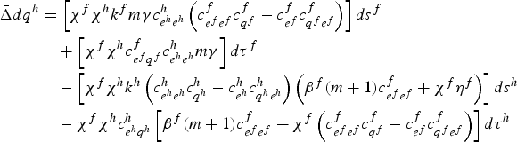 $$\eqalign{\bar{\Delta}d q^h & = \left[\chi ^{f}\chi ^{h}k^{f}m\gamma c^h_{e^h e^h}\left(c^f_{e^f e^f}c^f_{q^f}-c^f_{e^f}c^f_{q^f e^f}\right)\right]d s^f \cr & \quad +\left[\chi ^{f}\chi ^{h}c^f_{e^f q^f}c^h_{e^h e^h}m\gamma \right]d\tau^f \cr & \quad - \left[\chi ^{f}\chi ^{h}k^{h}\left(c^h_{e^h e^h}c^h_{q^h}-c^h_{e^h}c^h_{q^h e^h}\right)\left(\beta^f{\lpar m+1\rpar c^f_{e^f e^f}+\chi ^{f}\eta ^{f}}\right)\right]d s^h \cr & \quad -\chi ^{f}\chi ^{h}c^h_{e^h q^h}\left[\beta^f{\lpar m+1\rpar c^f_{e^f e^f}+\chi ^{f}\left(c^f_{e^f e^f}c^f_{q^f}-c^f_{e^f}c^f_{q^f e^f}\right)}\right]d\tau^h }$$
where the determinant of the coefficient matrix is
 $\bar{\Delta} \lt 0$
, the term c
z
e
z
e
z
c
z
q
z
− c
z
e
z
c
z
q
z
e
z
> 0 denotes marginal production costs and χ
z
= (1 − s
z
)k
z
> 0 for z = h, f, ω = β
h
β
f
(n + 1)(m + 1)− nmγ2 > 0, η
f
= c
f
e
f
e
f
c
f
q
f
q
f
− (c
f
e
f
q
f
)2 > 0 by the concavity of the c(·) function.Footnote
9
The analysis indicates that an increase in the subsidy in the home country raises (lowers) output in the home (foreign) country. This is because the subsidy in the home country renders firms operating in the home (foreign) country more (less) cost competitive via lower (higher) marginal production costs. In addition, an increase in the tax in the home country lowers (raises) output in the home (foreign) country because the tax renders home (foreign) firms less (more) cost competitive. Notice that as products become more differentiated (decrease in γ) the cross effect of policy becomes negligible since differences in cost competitiveness become small with more differentiated products. The effect of the policy on emissions is analyzed next.
$\bar{\Delta} \lt 0$
, the term c
z
e
z
e
z
c
z
q
z
− c
z
e
z
c
z
q
z
e
z
> 0 denotes marginal production costs and χ
z
= (1 − s
z
)k
z
> 0 for z = h, f, ω = β
h
β
f
(n + 1)(m + 1)− nmγ2 > 0, η
f
= c
f
e
f
e
f
c
f
q
f
q
f
− (c
f
e
f
q
f
)2 > 0 by the concavity of the c(·) function.Footnote
9
The analysis indicates that an increase in the subsidy in the home country raises (lowers) output in the home (foreign) country. This is because the subsidy in the home country renders firms operating in the home (foreign) country more (less) cost competitive via lower (higher) marginal production costs. In addition, an increase in the tax in the home country lowers (raises) output in the home (foreign) country because the tax renders home (foreign) firms less (more) cost competitive. Notice that as products become more differentiated (decrease in γ) the cross effect of policy becomes negligible since differences in cost competitiveness become small with more differentiated products. The effect of the policy on emissions is analyzed next.
Define global emissions as E = ne h + me f . Then, the effect of policy on emissions in the home country, e h , and foreign country, e f , are given by
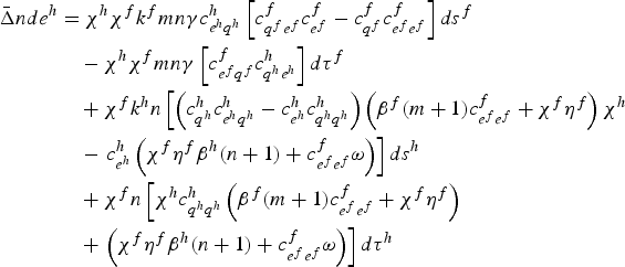 $$\eqalign{\bar{\Delta}nde^{h} &= \chi^{h} \chi ^{f} k^f mn \gamma c^h_{e^h q^h}\left[c^f_{q^f e^f} c^f_{e^f}-c^f_{q^f}c^f_{e^f e^f}\right]d s^f \cr & \quad - {\chi ^{h}\chi ^{f}mn\gamma \left[c^f_{e^f q^f}c^h_{q^h e^h}\right]d\tau^f} \cr & \quad +\chi ^{f}k^h n\left[\left(c^h_{q^h}c^h_{e^h q^h}-c^h_{e^h}c^h_{q^h q^h}\right)\left(\beta^f{\lpar m+1\rpar c^f_{e^f e^f}+\chi ^{f}\eta ^{f}}\right)\chi^{h}\right. \cr & \quad - \left.c^h_{e^h}\left(\chi ^{f}\eta ^{f}\beta^h\lpar n+1\rpar +c^f_{e^f e^f}\omega \right)\right]d s^h \cr & \quad +\chi ^{f}n\left[\chi ^{h}c^h_{q^h q^h}\left(\beta^f{\lpar m+1\rpar c^f_{e^f e^f}+\chi ^{f}\eta ^{f}}\right)\right. \cr & \quad + \left.\left(\chi ^{f}\eta ^{f}\beta^h\lpar n+1\rpar +c^f_{e^f e^f}\omega \right)\right]d\tau^h}$$
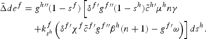
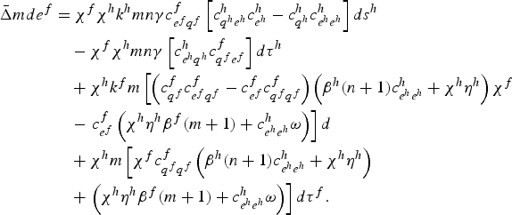 $$\eqalign{\bar{\Delta}md e^f &= \chi ^{f}\chi ^{h}k^h mn\gamma c^f_{e^f q^f}\left[c^h_{q^h e^h}c^h_{e^h} -c^h_{q^h}c^h_{e^h e^h}\right]d s^h \cr & \quad -\chi ^{f}\chi ^{h}mn\gamma \left[c^h_{e^h q^h}c^f_{q^f e^f}\right]d\tau^h \cr & \quad +\chi ^{h}k^f m\left[\left(c^f_{q^f}c^f_{e^f q^f}-c^f_{e^f}c^f_{q^f q^f}\right)\left(\beta^h\lpar n+1\rpar c^h_{e^h e^h}+\chi ^{h}\eta ^{h}\right)\chi^{f}\right. \cr & \quad - \left. c^f_{e^f}\left(\chi ^{h}\eta ^{h}\beta^f{\lpar m+1\rpar +c^h_{e^h e^h}\omega}\right)\right]d \cr & \quad +\chi ^{h}m\left[\chi ^{f}c^f_{q^f q^f}\left(\beta^h\lpar n+1\rpar c^h_{e^h e^h}+\chi^{h}\eta ^{h}\right)\right. \cr & \quad + \left.\left(\chi ^{h}\eta ^{h}\beta^f{\lpar m+1\rpar +c^h_{e^h e^h}\omega }\right)\right]d\tau^ f.}$$
Consider a policy reform where the home country raises the subsidy unilaterally (i.e., a policy reform such that ds
h
> 0). Using (6) it can be shown that emissions in the home country fall, if the pollution intensity coefficient in the home country is sufficiently small, i.e., if c
h
q
h
c
h
q
h
e
h
− c
h
e
h
c
h
q
h
q
h
> 0. Intuitively, there are two opposing effects at play here. On the one hand, the subsidy lowers marginal production costs, thereby increasing output (and therefore emissions); on the other, the subsidy lowers marginal abatement costs and so emissions fall as a result. Thus, if the country raising the subsidy has a small pollution intensity coefficient, then the increase in emissions is completely offset by the reduction in marginal abatement costs. As a special case, consider a cost function of the end-of-pipe such that c
z
=
![]() z
(q
z
) + g
z
(δ
z
(q
z
) − e
z
) where
z
(q
z
) + g
z
(δ
z
(q
z
) − e
z
) where
![]() z′ > 0,
z′ > 0,
![]() z″> 0, g
z′ > 0, g
z″ > 0, δ
z″ > 0, δ
z′ > 0, for z = f,h; the function δ
z
(·) denotes gross pollution and δ
z′ the pollution intensity coefficient.Footnote
10
Emissions in the home country fall if 0 < c
h
q
h
c
h
q
h
e
h
−c
h
e
h
c
h
q
h
q
h
= −g
h ″
z″> 0, g
z′ > 0, g
z″ > 0, δ
z″ > 0, δ
z′ > 0, for z = f,h; the function δ
z
(·) denotes gross pollution and δ
z′ the pollution intensity coefficient.Footnote
10
Emissions in the home country fall if 0 < c
h
q
h
c
h
q
h
e
h
−c
h
e
h
c
h
q
h
q
h
= −g
h ″
![]() h ′ δ
h ′ + δ
h ′
g
h ′ (
h ′ δ
h ′ + δ
h ′
g
h ′ (
![]() h ″ + g
h ″δ
h ″) , i.e., small intensity coefficient. If δ
h″ =0 and
h ″ + g
h ″δ
h ″) , i.e., small intensity coefficient. If δ
h″ =0 and
![]() h″ = 0, emissions in the home country fall if and only if −δ
h′
g
h ″
h″ = 0, emissions in the home country fall if and only if −δ
h′
g
h ″
![]() ^h ′β
f
(m + 1)χ
h
+ g
h ′ω > 0; this is a necessary and sufficient condition under which emissions in the home country fall. Footnote
11
This result applies to the cases where γ ≃ 0 and β
h
= β
f
= γ.
^h ′β
f
(m + 1)χ
h
+ g
h ′ω > 0; this is a necessary and sufficient condition under which emissions in the home country fall. Footnote
11
This result applies to the cases where γ ≃ 0 and β
h
= β
f
= γ.
As for the impact on emissions in the foreign country, using (7) the analysis indicates that with the policy reform ds h > 0 emissions in the foreign country fall unambiguously since c h q h e h c h e h − c h q h c h e h e h > 0. The intuition is that the subsidy in the home country renders firms operating in the foreign country less cost competitive, which reduces output and emissions in the foreign country. Notice that as products become more differentiated (decrease in γ ), the cross effect is negligible since differences in cost competitiveness become small.
The analysis suggests that the unilateral increase in the subsidy in the home country reduces global emissions, if the pollution intensity coefficient in the foreign country is relatively large. Intuitively, with a large pollution intensity coefficient in the foreign country, the reduction in emissions in that country (arising from the reduction in output in that country) as well as the reduction in emissions in the home country (via lower marginal abatement costs in that country) completely offset any increase in emissions in the home country. In the case of an end-of-pipe cost function as previously specified, global emissions fall, if δ
f′
mγ >δ
h′(β
f
(m + 1) + χ
f
(c
f ″ + g
f′δ
f″)). In the special case where
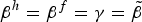 $\beta^h=\beta^f=\gamma =\tilde{\beta}$
, δ
f ″ = 0,
$\beta^h=\beta^f=\gamma =\tilde{\beta}$
, δ
f ″ = 0,
![]() f″ = 0, this condition simplifies to δ
f′
m > δ
h′(m + 1). Thus, assuming a fixed level of environmental R&D, global emissions fall with the unilateral increase in the subsidy in that country with a relatively small pollution intensity coefficient. Notice that with more differentiated products global emissions are likely to fall by less since differences in cost competitiveness become small.Footnote
12
In the case where γ ≃ 0, global emissions rise if and only if δ
h′β
f
(m + 1)> g
h′ω/
f″ = 0, this condition simplifies to δ
f′
m > δ
h′(m + 1). Thus, assuming a fixed level of environmental R&D, global emissions fall with the unilateral increase in the subsidy in that country with a relatively small pollution intensity coefficient. Notice that with more differentiated products global emissions are likely to fall by less since differences in cost competitiveness become small.Footnote
12
In the case where γ ≃ 0, global emissions rise if and only if δ
h′β
f
(m + 1)> g
h′ω/
![]() h′ χ
h
g
h″ (large intensity coefficient); that is, if the effect through marginal production costs (and therefore output) offsets the effect via marginal abatement costs.
h′ χ
h
g
h″ (large intensity coefficient); that is, if the effect through marginal production costs (and therefore output) offsets the effect via marginal abatement costs.
Proposition 3.1
Let the c (·, ·) function be of the end-of-pipe. Then assuming a fixed level of environmental R&D, global emissions fall with the unilateral increase in the subsidy in the home country if the foreign country is the pollution-intensive country, i.e., δ
f′γm > γ
h′β
f
(m + 1) + χ
f
(
![]() f″ + g
f′γ
f″).
f″ + g
f′γ
f″).
One policy implication of this result is that it proposes a unilateral reform for the pollution-moderate country which leads to lower global emissions.Footnote 13
Next, consider the policy reform d s
h
= d s
f
> 0 under an end-of-pipe cost function where δ
z″ = 0 and c
z″ = 0 for z = h, f. The multilateral increase in the subsidy reduces global emissions, if the pollution intensity coefficient in the foreign country is relatively small (i.e., δ
h′
nγ > β
h
(n + 1)δ
f′), so that the increase in the subsidy in the foreign country (the pollution-moderate country) reduces global emissions, and the pollution intensity coefficient in the home country is sufficiently small (i.e., δ
h′
nβ
f
(m + 1) < ωng
h′/
![]() h′ χ
h
g
h″) so that the increase in the subsidy in the home country lowers global emissions.Footnote
14
One policy implication here is that global emissions may fall if both the pollution-intensive and pollution-moderate country use R&D subsidies to promote pollution abatement. If γ ≃ 0, then global emissions also fall if the pollution intensity coefficient in each country is small.Footnote
15
This is because in the case of complete product differentiation the reduction in pollution via differences in cost competitiveness is negligible.
h′ χ
h
g
h″) so that the increase in the subsidy in the home country lowers global emissions.Footnote
14
One policy implication here is that global emissions may fall if both the pollution-intensive and pollution-moderate country use R&D subsidies to promote pollution abatement. If γ ≃ 0, then global emissions also fall if the pollution intensity coefficient in each country is small.Footnote
15
This is because in the case of complete product differentiation the reduction in pollution via differences in cost competitiveness is negligible.
Using (4) the policy reform ds
h
= dτ
h
/τ
h
> 0 is now examined.Footnote
16
Assuming a cost function of the end-of-pipe the analysis indicates that emissions in the foreign country fall\ if and only if
![]() h′
k
h
− δ
h′ > 0, where the first term captures the effect of the subsidy and the second the effect of the tax. To see the intuition behind this result, recall that an increase in the subsidy in the home country lowers emissions in the foreign country unambiguously; on the other hand, an increase in the tax in the home country raises (lowers) emissions in the foreign (home) country. Thus, from a potentially revenue-neutral policy in the home country, a unilateral increase in the subsidy and tax in that country reduces emissions in the foreign country if the effect via the tax is small.
h′
k
h
− δ
h′ > 0, where the first term captures the effect of the subsidy and the second the effect of the tax. To see the intuition behind this result, recall that an increase in the subsidy in the home country lowers emissions in the foreign country unambiguously; on the other hand, an increase in the tax in the home country raises (lowers) emissions in the foreign (home) country. Thus, from a potentially revenue-neutral policy in the home country, a unilateral increase in the subsidy and tax in that country reduces emissions in the foreign country if the effect via the tax is small.
Under the same policy reform the analysis suggests that global emissions fall, if γmδ
f′ < β
f
(m + 1)δ
h′ < β
f
(m + 1)g
h′/χ
h
![]() h′
g
h″. This condition says that if the home country is the pollution-intensive country (first inequality) the own effect of the tax dominates the cross effect, thereby lowering global emissions. At the same time, a sufficiently small pollution intensity coefficient in the home country (second inequality) results in a reduction in emissions in the home country via the subsidy. For completeness, in the case of complete product differentiation (γ ≃0) global emissions are more likely to fall with policy reform ds
h
= dτ
h
/τ
h
> 0, provided that the pollution intensity coefficient in the home country is sufficiently small, i.e., the second inequality holds. If instead ds
h
< 0 and dτ
h
> 0, then global emissions fall if the home country is the pollution-intensive country and δ
h′ > g
h′/χ
h
h′
g
h″. This condition says that if the home country is the pollution-intensive country (first inequality) the own effect of the tax dominates the cross effect, thereby lowering global emissions. At the same time, a sufficiently small pollution intensity coefficient in the home country (second inequality) results in a reduction in emissions in the home country via the subsidy. For completeness, in the case of complete product differentiation (γ ≃0) global emissions are more likely to fall with policy reform ds
h
= dτ
h
/τ
h
> 0, provided that the pollution intensity coefficient in the home country is sufficiently small, i.e., the second inequality holds. If instead ds
h
< 0 and dτ
h
> 0, then global emissions fall if the home country is the pollution-intensive country and δ
h′ > g
h′/χ
h
![]() h′
g
h″, i.e., the effect of the tax and subsidy, separately, reduce global emissions.
h′
g
h″, i.e., the effect of the tax and subsidy, separately, reduce global emissions.
The special case where ds
h
> 0 and dτ
h
/τ
h
< 0, γ ≃ 0 and c(·, ·) is a function of the end-of-pipe where δ
z″ = 0 and
![]() z″ = 0, suggests that if 1 > k
h
g
h′, then global emissions fall if and only if δ
h′ χ
h
g
h″(
z″ = 0, suggests that if 1 > k
h
g
h′, then global emissions fall if and only if δ
h′ χ
h
g
h″(
![]() h′χ
h
+ δ
h′) <β
h
(n + 1)(1 − k
h
g
h′).Footnote
17
This is because the effect of policy on emissions in the foreign country vanishes with γ ≃ 0, and a small pollution intensity coefficient helps offset any increases in emissions arising from the increase in the subsidy and decrease in the tax. If instead β
z
≥ γ and an analogous (sufficient) condition for δ
h′ holds (i.e., intensity coefficient is small), then global emissions also fall since emissions in the foreign country fall with a decrease in τ
h
and an increase in s
h
.
h′χ
h
+ δ
h′) <β
h
(n + 1)(1 − k
h
g
h′).Footnote
17
This is because the effect of policy on emissions in the foreign country vanishes with γ ≃ 0, and a small pollution intensity coefficient helps offset any increases in emissions arising from the increase in the subsidy and decrease in the tax. If instead β
z
≥ γ and an analogous (sufficient) condition for δ
h′ holds (i.e., intensity coefficient is small), then global emissions also fall since emissions in the foreign country fall with a decrease in τ
h
and an increase in s
h
.
This section concludes by looking at the policy reform dτ h /τ h = ds f > 0. Under the assumption of an end-of-pipe cost function as previously specified, if the home country is the pollution-intensive country and the foreign country the pollution-moderate country (i.e., δ h′ n> δ f′(n + 1)), then global emissions fall. The reason is that the decrease in emissions in the home country (due to the tax) completely offsets any increase in emissions in the foreign country, and the subsidy in the foreign country leads to lower global emissions because of the small pollution intensity coefficient in that country. This policy reform illustrates how different policies implemented across countries (perhaps a tax is more viable in one country whereas the subsidy is viable in other countries) reduce global emissions.
Proposition 3.2
Let the c(·,·) function be of the end-of-pipe where δ
z″ = 0 and c
z″ = 0 for z = h, f. Assume a fixed level of environmental R&D and let the foreign country be the pollution-moderate country and the home country the pollution-intensive country, i.e., δ
h′γ n > δ
f′βf(n + 1). Then, global emissions fall with an increase and decrease in the tax and subsidy, respectively, in the pollution-intensive country if the intensity coefficient in the pollution intensive country is large, i.e., δ
h′
n > g
h′/χ
h′
g
h″
![]() h′. Also, if the pollution-intensive country raises the tax and the pollution-moderate country raises the subsidy multilaterally (i.e., dτh/τh = ds
f
> 0), global emissions fall.
h′. Also, if the pollution-intensive country raises the tax and the pollution-moderate country raises the subsidy multilaterally (i.e., dτh/τh = ds
f
> 0), global emissions fall.
3.1.1. An illustrative example
To underscore some of the results previously presented and pave the way for the analysis in the next section, this section considers the special case where there is one firm in each country (i.e., m = n = 1) and the cost function is given by c(q,e) =
![]() q + (dq − e)2/2,
q + (dq − e)2/2,
![]() > 0. The term dq − e = a denotes units of pollution abated, a, and d is a constant which denotes the pollution intensity coefficient. In the context of the previous section g(·) = (dq − e)
2
/2, δ′ = d, δ″ = 0,
> 0. The term dq − e = a denotes units of pollution abated, a, and d is a constant which denotes the pollution intensity coefficient. In the context of the previous section g(·) = (dq − e)
2
/2, δ′ = d, δ″ = 0,
![]() ″ = 0, g
′ = a = dq − e and g
″ = 1. The model is first solved and some of the comparative statics results are underscored.
″ = 0, g
′ = a = dq − e and g
″ = 1. The model is first solved and some of the comparative statics results are underscored.
Maximization of (1) with respect to q h and e h yields
 $$\alpha^{h}-2\beta^h q^h-\gamma q^f-\lpar 1-s^h\rpar k^h\lpar \tilde{c}^{h}+a^h d^{h} \rpar = 0 $$
 $$\lpar 1-s^h\rpar k^h a^h-\tau^h= 0.$$
Using these and analogous expressions for the foreign country gives
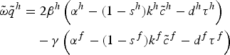 $$\eqalign{\tilde{\omega}\tilde{q}^{h} &= 2\beta^h \left(\alpha^h-\lpar 1-s^h\rpar k^h \tilde{c}^{h} - d^{h} \tau^h\right)\cr & \quad -\gamma \left(\alpha^f-\lpar 1-s^f\rpar k^f \tilde{c}^{f}-d^f\tau^f\right)}$$
 $$\tilde{e}^{h} = d^{h} \tilde{q}^{h}-{\tau^{h} \over \lpar 1-s^h\rpar k^h}\comma \; $$
where the last term in (11) denotes pollution abatement and
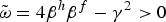 $\tilde{\omega} = 4\beta^h \beta^f - \gamma ^{2}\gt0$
.Footnote
18
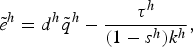
Notice that output in the home country falls (rises) with the level of R&D in the foreign (home) country since R&D renders firms less (more) cost competitive. In the special case where the level of environmental R&D is fixed, the effect of the subsidy and tax on emissions is given by
$\tilde{\omega} = 4\beta^h \beta^f - \gamma ^{2}\gt0$
.Footnote
18
Notice that output in the home country falls (rises) with the level of R&D in the foreign (home) country since R&D renders firms less (more) cost competitive. In the special case where the level of environmental R&D is fixed, the effect of the subsidy and tax on emissions is given by
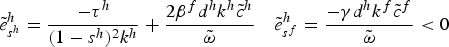 $$\tilde{e}_{s^h}^{h} = {-\tau^h \over \lpar 1-s^h\rpar ^{2}k^h}+{2\beta^f d^h k^h \tilde{c}^{h} \over \tilde{\omega}} \quad \tilde{e}_{s^f}^{h}={-\gamma d^h k^f \tilde{c}^{f}\over \tilde{\omega}} \lt 0 $$
 $$\tilde{e}_{\tau^h}^{h} = {-1 \over \lpar 1-s^h\rpar k^h} - {2\beta^f \lpar d^h\rpar ^2\over \tilde{\omega}} \lt 0 \quad \tilde{e}_{\tau^f}^{h}={d^h d^f \gamma \over \tilde{\omega}} \gt 0. $$
From (12) and (13), and analogous expressions for the foreign country, some of the results derived in the previous section, where it is assumed that policy changes do not work via R&D, can be underscored. For instance, a unilateral increase in the subsidy in the home country, s
h
, lowers emissions in that country if the reduction via lower marginal abatement costs offsets increases in emissions via more output; this occurs if and only if the pollution intensity coefficient is sufficiently small, i.e.,
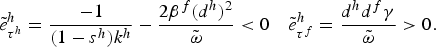
 $d^{h} \lt \tau^h \tilde{\omega}/2 \beta^f\lpar 1-s^h\rpar k^h \tilde{c}^{h}$
.Footnote
19
In addition, this policy reduces global emissions if the foreign country is the pollution-intensive country (i.e., d
f
γ > β
h
d
h
); this is because the reduction in output in the foreign country (and emissions in that country) offsets increases in emissions in the home country because of the relatively small intensity coefficient. These results are analogous to those presented in the previous section. Furthermore, the effect of an increase in the subsidy in the home country on global emissions, E = e
h
+ e
f
, is given by
$d^{h} \lt \tau^h \tilde{\omega}/2 \beta^f\lpar 1-s^h\rpar k^h \tilde{c}^{h}$
.Footnote
19
In addition, this policy reduces global emissions if the foreign country is the pollution-intensive country (i.e., d
f
γ > β
h
d
h
); this is because the reduction in output in the foreign country (and emissions in that country) offsets increases in emissions in the home country because of the relatively small intensity coefficient. These results are analogous to those presented in the previous section. Furthermore, the effect of an increase in the subsidy in the home country on global emissions, E = e
h
+ e
f
, is given by
 $$E_{s^h} = \tilde{e}_{s^h}^{h} + \tilde{e}_{s^h}^{f} = {-\tau^h \over \lpar 1-s^h\rpar ^{2}k^h} + {k^h \tilde{c}^{h} \over \tilde{\omega}} \left(2\beta^f d_{h} -\gamma d^f \right)\lt 0\comma \; ifd^f \gamma \gt \beta^h d^h$$
where global emissions fall with a unilateral increase in the subsidy in the home country, if the home country is the pollution-moderate country and the foreign country the pollution-intensive country (see proposition 3.1). Substituting (10) and (11) back into (1) and differentiating with respect to the level of R&D in the home country yields the following first-order condition: π h kh = −γ q h q f k h − (1 − s h )c h = 0, where the first term denotes the strategic effect and the second the cost reduction effect. Substituting the expressions for c h and q f k h and using (8) and (9) gives
 $$\tilde{q}^{h}\lpar k^h\rpar ^{2}={\lpar \tau^h\rpar ^{2}\tilde{\omega}\over 4 \beta^h \beta^f \tilde{c}^h \beta^f} \Rightarrow \lpar k^h\rpar ^{3}\zeta _{1}+\lpar k^h\rpar ^{2}\zeta _{2}-{\lpar \tau^h\rpar ^{2} \tilde{\omega}\over 8 \beta^h \beta^f \tilde{c}^h \beta^f}=0$$
where ζ1 and ζ2 are expressions of parameter values, the subsidy and tax in each country.Footnote 20 Under certain parameter values it can be shown that the roots to the polynomial may rise or fall with policy variables, thus showing a myriad of cases where policy changes affect emissions via environmental R&D. Important examples include k h s h > 0, k h s f < 0, k f s h < 0 and k f s f > 0. Some of these cases are taken up in the next section. For completeness, it is noted that the solution to the model is obtained by substituting the solution to k h and k f back into (10) and (11).
3.2. Effects through environmental R&D
This section analyzes multilateral and unilateral policy reform under the assumption that the subsidy or tax in one country affects the level of environmental R&D used by firms operating in that country as well as the other country.Footnote
21
As a result, there is an extra channel through which output, abatement efforts and emissions in each country might be impacted. The general policy implication derived in this section is that emissions fall if the pollution intensity coefficient is small in the country which experiences an increase in R&D with any given policy reform, and large in the country where R&D falls with policy. The analysis in this section proceeds under the assumption of a cost function of the end-of-pipe where δ
z″ = 0 and
![]() z″ = 0; z = h, f.
z″ = 0; z = h, f.
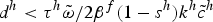
Consider the policy reform d s h > 0 and its impact on emissions in the home country in the case where the subsidy induces more environmental R&D in the home country, k h s h < 0, but lowers it in the foreign country, k f s h > 0. First, from the previous section recall that the direct effect of the subsidy (i.e., for given level of R&D) lowers production and abatement costs and, as a result, emissions in that country fall (rise) if the pollution intensity coefficient in the home country is small (large) enough. Second, since policy induces more R&D in the home country then production costs fall and therefore output and emissions rise in that country, and at the same time marginal abatement costs fall thereby lowering emissions. In this case the effect via R&D simply compensates the direct effect of the subsidy. Additionally, since R&D in the foreign country falls, then production costs in that country rise and therefore (via the oligopolistic interdependence captured by the parameter γ) home firms become more cost competitive thereby raising output and emissions in the home country further. As a result, emissions in the home country rise with the subsidy if and only if the intensity coefficient in the home country is large. Even though this case illustrates the possibility of increased emissions when the subsidy induces environmental R&D, it also underscores the case where the subsidy may reduce emissions in a country with a small enough intensity coefficient. The impact of s h on e h is given by
 $$\eqalign{\bar{\Delta}de^{h} &= g^{f \prime \prime }\chi ^{f} \left[\mu ^{h}\left(-\delta ^{h \prime }g^{h \prime \prime }\chi^{h}\beta^f{\lpar m+1\rpar }\tilde{c}^{h \prime} + \chi^{f}\beta^f g^{h \prime} g^{f \prime \prime } \omega \right)\right. \cr & \quad \left. - \delta ^{h \prime } \tilde{c}^{f \prime }g^{h \prime \prime }\chi ^{h}m\gamma \lpar 1-s^f\rpar k^{f}_{s^{h}}\right]ds^h}$$
where
 $\bar{\Delta}\lt0$
,
$\bar{\Delta}\lt0$
,
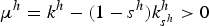 $\mu ^{h}=k^h-\lpar 1-s^h\rpar k^h_{s^h}\gt0$
captures the (net) effect of policy via R&D in the home country as well as the direct effect, and the second term the effect via R&D in the foreign country. The result derived in the preceding paragraph is stated more formally: emissions in the home country rise if and only if g
h′
g
f″ω μ
h
< δ
h′χ
h
g
h″(μ
h
β
f
(m + 1)
$\mu ^{h}=k^h-\lpar 1-s^h\rpar k^h_{s^h}\gt0$
captures the (net) effect of policy via R&D in the home country as well as the direct effect, and the second term the effect via R&D in the foreign country. The result derived in the preceding paragraph is stated more formally: emissions in the home country rise if and only if g
h′
g
f″ω μ
h
< δ
h′χ
h
g
h″(μ
h
β
f
(m + 1)
![]() h′ +
h′ +
![]() f ′ β
f
k
f
s
h
(1 − s
f
)mγ). It is noteworthy that this result holds as long as μ
h
> 0; this means that the result follows through even in the case where there is small decrease in R&D in the home country arising from the subsidy in that country (i.e., k
h
s
h
< k
h
/(1 − s
h
) or equivalently k
h
s
h
> 0 but small). However, if k
f
s
h
< 0 and k
h
s
h
> 0 is large so that μ
h
< 0 (i.e., the effect of the subsidy via k
h
offsets the direct effect), then emissions fall with an increase in the subsidy if the intensity coefficient in the home country is large. The intuition is that e
h
falls via k
f
s
h
< 0 and, in addition, e
h
falls via k
h
s
h
> 0 since δ
h′ is large (e
h
falls with less R&D, k
h
, and large intensity coefficient because a large intensity coefficient offsets increased emissions from higher marginal abatement costs) and this effect offsets the direct effect of the subsidy since μ
h
< 0. Lastly, consider the case where the direct effect of the subsidy in the home country offsets the effect via R&D in that country so that μ
h
= 0. In this case the effect of policy works entirely via changes in the R&D in the foreign country.
f ′ β
f
k
f
s
h
(1 − s
f
)mγ). It is noteworthy that this result holds as long as μ
h
> 0; this means that the result follows through even in the case where there is small decrease in R&D in the home country arising from the subsidy in that country (i.e., k
h
s
h
< k
h
/(1 − s
h
) or equivalently k
h
s
h
> 0 but small). However, if k
f
s
h
< 0 and k
h
s
h
> 0 is large so that μ
h
< 0 (i.e., the effect of the subsidy via k
h
offsets the direct effect), then emissions fall with an increase in the subsidy if the intensity coefficient in the home country is large. The intuition is that e
h
falls via k
f
s
h
< 0 and, in addition, e
h
falls via k
h
s
h
> 0 since δ
h′ is large (e
h
falls with less R&D, k
h
, and large intensity coefficient because a large intensity coefficient offsets increased emissions from higher marginal abatement costs) and this effect offsets the direct effect of the subsidy since μ
h
< 0. Lastly, consider the case where the direct effect of the subsidy in the home country offsets the effect via R&D in that country so that μ
h
= 0. In this case the effect of policy works entirely via changes in the R&D in the foreign country.
If γ ≃ 0, the effect via k
f
vanishes and as a result emissions fall if and only if g
h′
g
f″χ
f
ω > δ
h′ βf(m + 1)
![]() h′ χ
h
β
f
g
h″) with k
h
s
h
< 0 (or k
h
s
h
> 0 but small). This indicates that, with differentiated products and in the case where R&D rises with the subsidy, emissions in the home country fall, if the intensity coefficient in that country is small. Intuitively, with a small intensity coefficient the increase in emissions is offset by lower marginal abatement costs. Analogously, in the same case of complete product differentiation, with k
h
s
h
> 0 and large so that μ
h
< 0, then emissions in the home country fall with a sufficiently large δ
h′, i.e., if and only if −δ
h′
g
h″
h′ χ
h
β
f
g
h″) with k
h
s
h
< 0 (or k
h
s
h
> 0 but small). This indicates that, with differentiated products and in the case where R&D rises with the subsidy, emissions in the home country fall, if the intensity coefficient in that country is small. Intuitively, with a small intensity coefficient the increase in emissions is offset by lower marginal abatement costs. Analogously, in the same case of complete product differentiation, with k
h
s
h
> 0 and large so that μ
h
< 0, then emissions in the home country fall with a sufficiently large δ
h′, i.e., if and only if −δ
h′
g
h″
![]() h′ βf(m + 1) + g
h′ω < 0.
h′ βf(m + 1) + g
h′ω < 0.
In contrast to the previous section, the impact of d s
h
> 0 on emissions in the foreign country is no longer unambiguous. In the case where k
f
s
h
> 0 and k
h
s
h
< 0, now the subsidy reduces environmental R&D in the foreign country and so output falls in that country, but marginal abatement costs rise. Additionally, emissions in the foreign country fall via the oligopolistic interdependence since k
h
s
h
< 0 (i.e., μ
h
> 0). As a result, emissions fall if the pollution intensity coefficient in the foreign country is sufficiently large. Intuitively, with a sufficiently large intensity coefficient, the reduction in emissions completely offsets the increase in emissions arising from higher marginal abatement costs. In particular, emissions in the foreign country fall, if δ
f′β
h
(n + 1) > g
f′ω /
![]() f′
g
f″χ
f
. The impact of s
h
on e
f
is given by
f′
g
f″χ
f
. The impact of s
h
on e
f
is given by
 $$\eqalign{\bar{\Delta}de^{f} &= g^{h \prime \prime }\lpar 1-s^f\rpar \left[\delta ^{f \prime}g^{f \prime \prime}\lpar 1-s^{h}\rpar \tilde{c}^{h\prime}\mu^{h} n\gamma \right. \cr & \quad \left. + k^f_{s^{h}}\left(\delta ^{f \prime } \chi^{f}\tilde{c}^{f \prime} g^{f \prime \prime}\beta^h\lpar n+1\rpar -g^{f \prime}\omega \right)\right]ds^h.}$$
In the case where γ ≃ 0 the effect via k
h
s
h
(as well as the direct effect of s
h
) vanishes and so emissions in the foreign country fall with the subsidy in the home country if and only if δ
f′ < g
f′β
f
(m + 1)/
![]() f′
g
f″ χ
f
) with k
f
s
h
< 0 or if and only if δ
f′ > g
f′ βf(m + 1)/
f′
g
f″ χ
f
) with k
f
s
h
< 0 or if and only if δ
f′ > g
f′ βf(m + 1)/
![]() f′
g
f″χ
f
with k
f
s
h
> 0. In the case where β
z
≥ γ, k
h
s
h
> 0 and k
f
s
h
> 0 emissions in the foreign country fall, if the effect of the subsidy via k
h
s
h
is sufficiently small (so that μ
h
> 0) and δ
f′ is sufficiently large. In this case e
f
falls via k
f
s
h
> 0 (since δ
f′ is large it offsets increased emissions from higher marginal abatement costs in the foreign country) and also because the direct effect of the subsidy (which reduces e
f
) offsets the effect via k
h
s
h
(which raises e
f
), i.e., μ
h
> 0. If k
f
s
h
< 0, k
h
s
h
> 0 and large (μ
h
< 0), then emissions fall if δ
f′ is sufficiently small. To see this, notice that in this case emissions in the foreign country rise because the direct effect of the subsidy is offset by the effect via k
h
(since μ
h
< 0), but fall via k
f
if the intensity coefficient is small enough. As a result, a small intensity coefficient, δ
f′, is required for emissions in the foreign country to fall.
f′
g
f″χ
f
with k
f
s
h
> 0. In the case where β
z
≥ γ, k
h
s
h
> 0 and k
f
s
h
> 0 emissions in the foreign country fall, if the effect of the subsidy via k
h
s
h
is sufficiently small (so that μ
h
> 0) and δ
f′ is sufficiently large. In this case e
f
falls via k
f
s
h
> 0 (since δ
f′ is large it offsets increased emissions from higher marginal abatement costs in the foreign country) and also because the direct effect of the subsidy (which reduces e
f
) offsets the effect via k
h
s
h
(which raises e
f
), i.e., μ
h
> 0. If k
f
s
h
< 0, k
h
s
h
> 0 and large (μ
h
< 0), then emissions fall if δ
f′ is sufficiently small. To see this, notice that in this case emissions in the foreign country rise because the direct effect of the subsidy is offset by the effect via k
h
(since μ
h
< 0), but fall via k
f
if the intensity coefficient is small enough. As a result, a small intensity coefficient, δ
f′, is required for emissions in the foreign country to fall.
In terms of global emissions, the analysis indicates that in the case where k
h
s
h
< 0 and k
f
s
h
> 0, global emissions fall with d s
h
> 0, if the foreign country is the pollution-intensive country (i.e., γ mδ
f′ > β
f
(m + 1)δ
h′) and the pollution intensity coefficient in that country is sufficiently large, i.e., g
f′ω + g
f″
![]() f′χ
f
γ nδ
h′ < g
f″
f′χ
f
γ nδ
h′ < g
f″
![]() f′ χ
f
β
h
(n + 1)δ
f′. The intuition is that the large pollution intensity coefficient in the foreign country (pollution-intensive country) offsets, on the one hand, increased emissions in the home country (pollution-moderate country) and, on the other, increased emissions in the foreign country arising from higher marginal abatement costs in that country.Footnote
22
Analogously, global emissions fall with a decrease in the subsidy if k
f
s
h
< 0, and k
h
s
h
> 0 and large (μ
h
< 0). The effect of d s
h
> 0 on global emissions, d E = nd e
h
+ md e
f
, is given by
f′ χ
f
β
h
(n + 1)δ
f′. The intuition is that the large pollution intensity coefficient in the foreign country (pollution-intensive country) offsets, on the one hand, increased emissions in the home country (pollution-moderate country) and, on the other, increased emissions in the foreign country arising from higher marginal abatement costs in that country.Footnote
22
Analogously, global emissions fall with a decrease in the subsidy if k
f
s
h
< 0, and k
h
s
h
> 0 and large (μ
h
< 0). The effect of d s
h
> 0 on global emissions, d E = nd e
h
+ md e
f
, is given by
 $$\eqalign{\bar{\Delta}dE &= g^{f \prime \prime }\chi ^{f}g^{h \prime \prime } \chi ^{h}\left[\mu ^{h}n\tilde{c}^{h \prime }\left(g^{h \prime } \omega /\chi ^{h}\tilde{c}^{h \prime }g^{h \prime \prime }+\gamma m\delta ^{f \prime }-\beta^f\lpar m+1\rpar \delta^{h \prime}\right)\right. \cr & \quad \left. + k^f_{s^h}\tilde{c}^{f \prime }m \left(-g^{f \prime }\omega / \chi ^{f}\tilde{c}^{f \prime }g^{f \prime \prime }+\beta^h\lpar n+1\rpar \delta ^{f \prime}-\gamma n\delta ^{h \prime }\right)\right]d s^h.}$$
In the case where γ ≃ 0 and under the assumption k
f
s
h
> 0 and k
h
s
h
< 0 global emissions fall, if the pollution intensity coefficient in the home and foreign country is sufficiently small and large, respectively, i.e., δ h ′ β
f
(m + 1) < g
h′/g
h″
![]() h′ χ
h
and δ
f′ β
h
(n + 1) > g
f′ /g
f″
h′ χ
h
and δ
f′ β
h
(n + 1) > g
f′ /g
f″
![]() f′ χ
f
.
f′ χ
f
.
Proposition 3.3
Let the c(·,·) function be of the end-of-pipe where δ z″ = 0, c z″ = 0. Assume that the foreign country is the pollution-intensive country, i.e., γ mδ f′ > βf(m + 1)δ h′. Then, a unilateral increase (decrease) in the subsidy in the pollution-moderate country lowers global emissions, if environmental R&D rises (falls) with the subsidy in the pollution-moderate country, falls (rises) in the pollution-intensive country and the pollution intensity coefficient in the pollution-intensive country is sufficiently large.
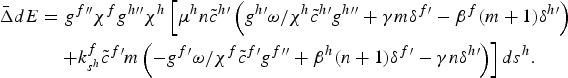
The policy reform ds h = dτ h /τ h > 0 is now examined. The effect of this policy on global emissions, dE = nde h + mde f , is given by
 $$\eqalign{\bar{\Delta}dE &=\nu \left[\psi ^{h}mn\tilde{c}^{h\prime }\lpar \delta ^{h\prime }\beta^f{-\delta ^{f \prime }\gamma \rpar +\psi ^{h}\left(n\tilde{ c}^{h \prime }\delta ^{h\prime }\beta^f -g^{h \prime }\omega /\lpar 1-s^h \rpar g^{h \prime \prime }\right)}\right. \cr &\quad \left. +\psi ^{f}mn\tilde{c}^{f \prime}\lpar \delta ^{f \prime }\beta^h -\delta ^{h \prime }\gamma \rpar +\psi ^{f}\left(m\tilde{c}^{f \prime } \delta ^{f \prime }\beta^h-g^{f \prime }\omega /\lpar 1-s^f\rpar g^{f \prime \prime }\right)\right. \cr &\quad +\left. g^{f \prime \prime }\lpar 1-s^f\rpar n\omega +\nu \lpar 1-s^h\rpar \lpar 1-s^f\rpar \delta ^{h}\left(\beta^f\lpar m+1\rpar \delta ^{h \prime }-\gamma m\delta ^{f \prime }\right)\right]\epsilon ^{h}}$$
where ψ
h
= (1 − s
h
)(k
h
τ
h
+ k
h
s
h
) − k
h
denotes the net effect of τ
h
and s
h
on the level of environmental R&D in the home country and ψ
f
= (1 − s
f
)(k
f
τ
h
+ k
f
s
h
) in the foreign country, and ν = g
f″
g
h″ (1 − s
h
)(1 − s
f
) > 0. The last term in (16) represents the direct effect of the tax. There is a myriad of possible cases so only a handful of cases are presented. The case where ψ
h
> 0 and ψ
f
< 0 indicates that the effect of policy reform raises environmental R&D in the foreign country and reduces it in the home country.Footnote
23
In this case and assuming that the home country is the pollution-intensive country (i.e., γδ
h′
n − β
h
(n + 1)δ
f′ > 0), if δ
h′
n > g
h′ω /g
h′(1 − s
h
)
![]() h′ and δ
f′
m < g
f′ ω/g
f′(1 − s
f
)
h′ and δ
f′
m < g
f′ ω/g
f′(1 − s
f
)
![]() f′, then global emissions fall with the policy reform d s
h
= dτ
h
/τ
h
> 0. The intuition is as follows. First, the direct effect of the tax lowers total emissions since the home country is the pollution-intensive country. Second, as R&D in the home country falls and rises in the foreign country, a relatively large intensity coefficient in the home country offsets any increase in emissions in the home country arising from higher marginal abatement costs in that country; a small intensity coefficient in the foreign country helps offset any increase in emissions in the foreign country arising from more R&D and lower production costs in that country.
f′, then global emissions fall with the policy reform d s
h
= dτ
h
/τ
h
> 0. The intuition is as follows. First, the direct effect of the tax lowers total emissions since the home country is the pollution-intensive country. Second, as R&D in the home country falls and rises in the foreign country, a relatively large intensity coefficient in the home country offsets any increase in emissions in the home country arising from higher marginal abatement costs in that country; a small intensity coefficient in the foreign country helps offset any increase in emissions in the foreign country arising from more R&D and lower production costs in that country.
In the case where ψ
f
< (>)0, ψ
h
> (<)0 and γ ≃ 0, if δ
h′ β
f
(m + 1) > (<)g
h′ω/g
h′(1 − s
h
)
![]() h′ and δ
f′ β
h
(n + 1) < (>)g
f′ω/g
f′(1 − s
f
)
h′ and δ
f′ β
h
(n + 1) < (>)g
f′ω/g
f′(1 − s
f
)
![]() f′, then global emissions fall. In this case differences in cost competitiveness vanish and as a result the conditions for lower emissions require a sufficiently large (small) and small (large) intensity coefficient in the home (foreign) and foreign (home) country.
f′, then global emissions fall. In this case differences in cost competitiveness vanish and as a result the conditions for lower emissions require a sufficiently large (small) and small (large) intensity coefficient in the home (foreign) and foreign (home) country.
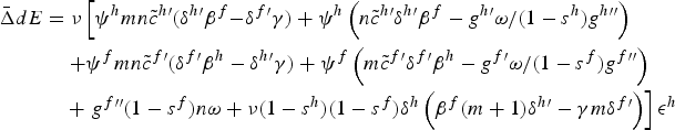
The role of the strategic variable is analogous in the context of the policy reform d s
h
= d s
f
= ds > 0. It can be shown that if ψ
f
> 0 and ψ
h
< 0, global emissions fall if the foreign country is the pollution-intensive country (i.e., δ
h′β
f
(m + 1) < δ
f′
mγ) and it has a relatively large intensity coefficient (g
f′ ω /g
f″
![]() f′(1 − s
f
) + δ
h′
nγ <δ
f′ β
h
(n + 1)). The intuition is that if policy lowers R&D in the foreign country and raises R&D in the home country, then a large pollution intensity coefficient in the foreign country offsets any increases in emissions. Analogously, a multilateral decrease in the subsidy reduces emissions, if ψ
f
< 0, ψ
h
> 0. For completeness, the effect of the policy reform d s
h
= d = s
f
ds > 0 is given by
f′(1 − s
f
) + δ
h′
nγ <δ
f′ β
h
(n + 1)). The intuition is that if policy lowers R&D in the foreign country and raises R&D in the home country, then a large pollution intensity coefficient in the foreign country offsets any increases in emissions. Analogously, a multilateral decrease in the subsidy reduces emissions, if ψ
f
< 0, ψ
h
> 0. For completeness, the effect of the policy reform d s
h
= d = s
f
ds > 0 is given by
 $$\eqalign{\bar{\Delta}dE &=\left[\tilde{\psi}^{f}\tilde{c}^{f \prime }m\nu \left(-g^{f \prime }\omega /g^{f \prime \prime }\tilde{c}^{f \prime }\lpar 1-s^f\rpar +\left(\delta ^{f \prime }\beta^h\lpar n+1\rpar -\delta ^{h \prime}n\gamma \right)\right)\right. \cr & \quad \left. +\tilde{\psi}^{h}\tilde{c}^{h \prime }n\nu \left(-g^{h \prime}\omega /g^{h \prime \prime }\tilde{c}^{h \prime }\lpar 1-s^h\rpar +\left(\delta ^{h \prime }\beta^f{\lpar m+1\rpar -\delta ^{f \prime }m\gamma }\right)\right)\right]ds}$$
where ψ˜ h = (1 − s h )(k h s f + k h s h ) −k h and ψ˜ f = (1 − s f )( k f s h + k f s f ) −k f .
Proposition 3.4
Global emissions fall under different multilateral policy reforms and parameter values, if environmental R&D falls with the policy reform in the country which has a relatively large pollution intensity coefficient, but rises in the country which has a relatively small pollution intensity coefficient.
4. Policy reform and welfare analysis
This section looks at the impact of different policy reforms on welfare. These policy reforms can be thought of as multilateral efforts by countries to coordinate policy. The analysis proceeds by assuming that the initial values of the subsidy and tax are at the Nash equilibrium, which allows us to capture the international externalities of policy reform, the role of product differentiation and the inefficiencies arising from the non-cooperative equilibrium.Footnote 24 It is shown that, starting from the Nash equilibrium, an increase in the tax in, say, the foreign country raises welfare in the home country; and a decrease in the subsidy in the foreign country also raises welfare in the home country. A second but important result is that policy makers have more flexibility to implement different policy reforms to reduce global emissions in the case where products are very differentiated.
Ulph and Ulph (Reference Ulph, Ulph, Carraro, Katsoulacos and Xepapadeas1996, Reference Ulph and Ulph2007) and Katsoulacos and Xepapadeas (Reference Katsoulacos, Xepapadeas, Carraro, Katsoulacos and Xepapadeas1996) characterize the optimal emission tax and R&D subsidy under different scenarios, so the focus here is on the impact of policy reform on welfare. I shall follow Ulph and Ulph (Reference Ulph and Ulph2007) in the set-up of the welfare function because in this way clear-cut results are obtained and a connection to the characterization of policy in their model can be clearly established. In this case the emission tax finances subsidy payments and firms in each country export to a third country so that consumer surplus effects are not present.
Define welfare in the home country, W h , as total profits minus the damage from pollution; that is,
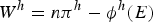 $$W^{h} = n\pi ^{h}-\phi ^{h}\lpar E\rpar $$
where E = n e h + m e f and the ϕ (·) function denotes damage from total pollution satisfying ϕ h′ >0, ϕ h″ > 0. An analogous expression applies to the foreign country, W f . Countries choose the emission tax and R&D subsidy non-cooperatively, taking the other country's policy as given. This yields four first-order conditions which implicitly determine the Nash equilibrium policy vector s h*, s f*, τ h*, τ f*.
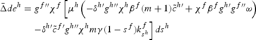
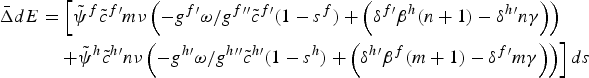
Differentiation of (18) and using the first-order conditions of home firms yields (see appendix for a derivation)
 $$\eqalign{dW^{h} &= \left[n \pi^h_{q^f}\left(q^f_{k^h}k^h_{s^f} +q^f_{k^f}k^f_{s^f} +q^f_{s^f} \right)-\phi^{h \prime }\left(E_{s^f} + E_{k^h}k^h_{s^f} +E_{k^f}k^f_{s^f}\right)\right]d s^f \cr &\quad + \left[n \pi^h_{q^f}\left(q^f_{k^h}k^h_{\tau^f} +q^f_{k^f}k^f_{\tau^f} +q^f _{\tau^f} \right)\right. \cr &\quad - \left.\phi^{h \prime}\left(E_{\tau^f} + E_{k^h}k^h_{\tau^f} +E_{k^f}k^f_{\tau^f}\right)\right]d\tau^f \cr &\quad + \left[n \pi^h_{q^f}\left(q^f_{k^h}k^h_{s^h} +q^f_{k^f}k^f_{s^h} +q^f_{s^h} \right)+n\pi^h_{s^h}\right. \cr &\quad - \left.\phi^{h \prime }\left(E_{s^h} + E_{k^h}k^h_{s^h} +E_{k^f}k^f_{s^h}\right)\right]d s^h \cr &\quad + \left[n \pi^h_{q^f}\left(q^f_{k^h}k^h_{\tau^h} +q^f_{k^f}k^f_{\tau^h} +q^f _{\tau^h} \right)+ n\pi^h_{\tau^h}\right. \cr &\quad - \left.\phi^{h \prime }\left(E_{\tau^h} + E_{k^h} k^h_{\tau^h} +E_{k^f}k^f_{\tau^h}\right)\right]d\tau^h }$$
where an analogous expression applies to W f and E denotes total emissions, ne h + me f . It is noteworthy that (19) captures the effect of policy via the strategic variable and that the third and fourth terms are equal to zero at the Nash equilibrium. This expression constitutes the backbone for the analysis that follows.
Consider a decrease in the subsidy in the foreign country starting from the Nash equilibrium. In the case where the level of R&D is fixed, so that k f s z = 0 and k h τ z = 0,z = h,f, or in the case where policy takes place via R&D (in particular if k f s f < 0 and k h s f > 0), it can be shown that a decrease in the subsidy in the foreign country raises welfare in the home country. In particular, using the foreign country's welfare first-order condition as well as (2) and (3), the impact of the foreign subsidy in the home country's welfare, starting from the Nash equilibrium, is given by (see the appendix for a derivation)
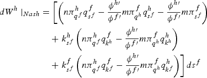 $$\eqalign{dW^{h}\mid_{Nash} &= \left[\left(n\pi^h_{q^f}q^f_{{s^f}}-{\phi ^{h \prime }\over \phi ^{f \prime }} m\pi^f_{q^h}q^h_{{s^f}}-{\phi ^{h \prime }\over \phi ^{f \prime }}m\pi^f_{{s^f}}\right)\right. \cr &\quad + \left. k^h_{{s^f}}\left(n\pi^h_{q^f}q^f_{k^h}- {\phi ^{h \prime }\over{\phi ^{f \prime }}}m\pi^f_{q^h}q^h_{k^h}\right)\right. \cr &\quad + \left. k^f_{{s^f}}\left(n\pi^h_{q^f}q^f_{k^f}-{\phi ^{h \prime }\over \phi ^{f \prime }} m\pi^f_{q^h}q^h_{k^f}\right)\right]d s^f}$$
where q f s f > 0, q h s f < 0, q f k f < 0, q h k f > 0, q h k h < 0, q f k h > 0, π h q f = −q h mγ <0, π f q h = −q f nγ <0, π f s f = k f c f (·) > 0. Notice that (20) captures the international externalities of the policy reform (since the initial values of policy are the Nash equilibrium) and the role of product differentiation. Additionally, the first term denotes the effect of the subsidy when policy does not work via R&D and the last two terms capture, respectively, the effect via R&D in the home and foreign country. There are two positive welfare effects in the first term which arise from the subsidy. On the one hand, a reduction in the subsidy in the foreign country raises profits in the home country (this is because foreign firms are less cost competitive which allows home firms to increase market share and profits) and, on the other, profits, output and emissions in the foreign country fall and, as a result, transboundary pollution falls. In the case where policy works via the strategic variable, welfare in the home country rises with a decrease in the subsidy in the foreign country, if k f s f < 0 and k h s f > 0; this case is in line with the ‘standard case’ in Ulph and Ulph (Reference Ulph and Ulph2007: 169). The intuition is that a decrease in R&D in the foreign country, resulting from a decrease in the subsidy in that country, lowers profits, output and therefore transboundary pollution and raises profits at home; and an increase in R&D in the home country raises profits in that country, and output and emissions in the foreign country fall, thereby lowering transboundary pollution. It is noteworthy that the effects of policy via the strategic variable of home firms and foreign firms could potentially offset each other, but additional assumptions about the k h and k f functions would be needed. The role of product differentiation is also clear from (20). In particular, as products become very differentiated (i.e., if γ ≃ 0, then π h q f and π f q h vanish), the cross effect of policy works via the effect of transboundary pollution, π f s f ϕ h′ /ϕ f′, since differences in cost competitiveness across countries are negligible: a reduction in the subsidy in the foreign country lowers profits, output and emissions in that country, thereby reducing transboundary pollution and raising welfare in the home country. This result is important because it indicates that the effect of policy reform on welfare becomes smaller with more differentiated products.
As a second case, consider a policy reform where the tax in the foreign country increases. In the case where changes in policy do not affect environmental R&D (i.e., k f τ z = 0 and k h τ z = 0,z = h,f) or if k f τf > 0 and k h τf < 0, welfare in the home country rises. Intuitively, an increase in the tax in the foreign country raises profits in the home country and lowers transboundary pollution (two positive welfare effects). In the case where environmental R&D in the home and foreign country, respectively, rises and falls with the tax in the foreign country the welfare effects are reinforced. In line with Ulph and Ulph (Reference Ulph and Ulph2007) I consider the case where R&D rises in each country given a tax increase in the foreign country, i.e., k f τf < 0 and k h τf < 0. In this case an increase in the tax in the foreign country raises profits at home and lowers transboundary pollution; but now an increase in the tax induces more R&D in the foreign country which raises emissions in that country and therefore transboundary pollution, and at the same time lowers profits in the home country. If the effect via changes in R&D in the foreign country is small, then welfare in the home country rises. This policy reform illustrates the inefficiencies from the non-cooperative equilibrium where international pollution externalities are not accounted for by each country. In the case where products are completely differentiated (γ ≃ 0), the cross effect works via the effect of transboundary pollution, ϕ h′/ϕ f′π f τf : an increase in the tax in the foreign country lowers profits, output, emissions and therefore transboundary pollution, which consequently raises welfare in the home country. Starting from the Nash equilibrium the impact on welfare in the home country is given by
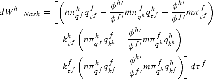 $$\eqalign{dW^{h}\mid_{Nash} &= \left[\left(n\pi^h_{q^f}q^f_{{\tau^f}}-{\phi ^{h \prime }\over \phi ^{f \prime }} m\pi^f_{q^h}q^h_{{\tau^f}}-{\phi ^{h \prime }\over \phi ^{f \prime }}m\pi^f_{{\tau^f}}\right)\right. \cr &\quad + \left. k^h_{{\tau^f}}\left(n\pi^h_{q^f}q^f_{k^h}- {\phi ^{h \prime }\over{\phi ^{f \prime }}}m\pi^f_{q^h}q^h_{k^h}\right)\right. \cr &\quad + \left. k^f_{{\tau^f}}\left(n\pi^h_{q^f}q^f_{k^f}-{\phi ^{h \prime }\over \phi ^{f \prime }} m\pi^f_{q^h}q^h_{k^f}\right)\right]d \tau^f}$$
where π f τ f = −e f < 0.
Proposition 4.1
Starting from the Nash equilibrium, an increase (decrease) in the emission tax (R&D subsidy) in one country raises welfare in the other country when R&D is fixed. In the case where policy works via changes in environmental R&D, an increase (decrease) in the tax (subsidy) in one country raises welfare in the other country, if the tax (subsidy) decreases (increases) R&D in the country raising (lowering) the tax (subsidy) and increases (decreases) R&D in the other country.
Next, I examine a multilateral agreement of an equal increase in the tax and subsidy in the foreign country (i.e., d s f = dτ f /τ f > 0) in the case where policy does not work via the strategic variable and the cost function is of the end-of-pipe. Combining (20) and (21) yields
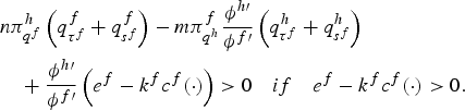 $$\eqalign{& n\pi^h_{q^f}\left(q^f_{\tau^f}+q^f_{{s^f}}\right)-m\pi^f_{q^h}{\phi ^{h \prime }\over \phi ^{f \prime }}\left(q^h_{\tau^f}+q^h_{{s^f}}\right)\cr &\quad + {\phi ^{h \prime }\over \phi ^{f\prime }}\left(e^f-k^f c^f\lpar{\cdot}\rpar \right)\gt 0 \quad if \quad e^f - k^f c^f \lpar{\cdot}\rpar \gt 0.}$$
Intuitively, an increase in the subsidy and tax in the foreign country raises welfare in the home country if the tax effect offsets the subsidy effect (i.e., e f > k f c f (· )) assuming that policy does not work via the strategic variable.Footnote 25 The idea here is that the tax (subsidy) effect raises (lowers) profits in the home country and lowers (raises) transboundary pollution and thus welfare in the home country rises if the tax effect is large. This result is important because it indicates that, along with the analysis in section 3.1, there exists a policy reform which could be implemented by the pollution-intensive country which may reduce global emissions and raise global welfare. This result follows through if k h s f + k h τ f < 0 and k f s f + k f τ f > 0, that is, if the subsidy and tax in the foreign country induces less R&D in that country, but induces more R&D in the home country. The intuition is that with less R&D in the foreign country and more R&D in the home country, transboundary pollution falls and profits in the home country rise, thereby raising welfare in that country.
This section concludes by looking at a multilateral agreement where the subsidy is increased (in order to promote environmental R&D) and then governments are free to adjust their emission tax subsequently so as to keep tax revenue constant; this policy reform is important in those countries where the carbon tax may be an important source of revenue.Footnote 26 The implication here is that the adjustment in the tax adds a channel whereby policy reform may impact welfare. In this policy reform, total differentiation of the tax revenue in the foreign country, τ f E f , gives
 $$0=\lpar E^{f}+\tau^f E_{\tau^f}^{f}\rpar d\tau^f+\tau^f E_{{s^f}}^{f}d s^f{\quad \Rightarrow \quad d\tau^f/d s^f=-\tau^f E_{{s^f}}^{f}/E^{f}\lpar 1+\rho \rpar }$$
where ρ =(τ f /E f )E τ f f and 1 + ρ can assume a positive or negative value. In the case where the tax lowers tax revenue, τ f E f , so that 1 + ρ< 0, and the subsidy lowers emissions, an increase in the subsidy in the foreign country induces the government in that country to lower the tax. As a result and using proposition 4.1, welfare in the home country rises via the policy reform (d s f < 0) and the policy adjustment (dτ f /ds f < 0). In contrast, if the tax raises tax revenue and the subsidy lowers emissions, then with an increase in the subsidy the government adjusts the tax upwards, i.e., dτ f /ds f > 0; in this case and also under proposition 4.1, welfare in the home country may rise if the effect through the tax adjustment is large. The analysis illustrates the viability of a multilateral agreement where an increase in the subsidy in the pollution-moderate country may raise global welfare.
Proposition 4.2
Consider a multilateral agreement where the foreign and home country raise the subsidy, starting from the Nash equilibrium, while the government in each country adjusts the tax so that tax revenue remains constant. In the case where the tax raises tax revenue and the subsidy lowers emissions, global welfare rises if under proposition 4.1 the effect via the tax adjustment is large.
5. Conclusion
Emission taxes and subsidies to encourage environmental R&D are two widely used environmental policies. Examples of countries which have implemented these policies in a unilateral and multilateral fashion include Norway, The Netherlands and member countries in the Asia-Pacific Partnership on Clean Development and Climate; examples of industries where these policies have been implemented include the energy sector, a sector characterized by some degree of product differentiation. From a practical standpoint, different countries may deviate from the Nash equilibrium depending on the type of multilateral/unilateral agreements with other countries. In this context, the present analysis offers a systematic treatment of policy reform and its impact on global emissions and welfare. This type of analysis is new in the literature and so hopefully it will encourage future research in this area.
The comparative statics analysis suggests that unilateral and multilateral policy may reduce global emissions and raise welfare. The relative size of pollution intensity coefficients, degree of product differentiation and the effect of policy via R&D are key elements in the analysis. In particular, in the case where the level of R&D is fixed, the unilateral increase in the subsidy in the home country lowers global emissions if the country raising the subsidy is a pollution-moderate country. Secondly, global emissions fall if the pollution-intensive and pollution-moderate countries raise the subsidy multilaterally. Thirdly, the potentially revenue-neutral policy dτ h /τh = d s h > 0 lowers global emissions, if the country raising the tax and subsidy is the pollution-intensive country. In the case where policy changes take effect via R&D, the analysis indicates that there are a number of policy reforms under which global emissions fall if R&D falls in the pollution-intensive country and rises in the pollution-moderate country.
The nature of the model inevitably leaves out important analytical aspects of environmental policy and environmental R&D. For instance, the focus here is on quantity competition; aspects of quantity versus price competition are already present in the literature (e.g., Symeonidis, Reference Symeonidis2003). Second, to simplify the analysis no distinction was made about the type of R&D and issues of technology diffusion are assumed away (see, e.g., McGinty and de Vries (Reference McGinty and de Vries2009) for aspects of technology diffusion). Finally, many of the results depend crucially on the assumption that more and less R&D reduces and increases costs, respectively. Thus, a future venue of research would be to relax this assumption and see how results may change.
There are several issues which can be studied by extending the present model set-up. For instance, the role of free-entry could be explored by looking at how the subsidy, in the context of policy reform, may alter production incentives thereby increasing emissions in the long run. A combination of policies may also be incorporated into the analysis. For example, many industries may be facing not only a subsidy and tax, but also other policies such as emission standards or operating in an emissions permitting system. Additionally, the case of many countries with different size may yield interesting results since large countries may offset emission-reduction policies set by relatively small countries.
Appendix
This section presents the system utilized for the comparative statics analysis and analyzes policy reform. In particular, total differentiation of (2) and (3), and analogous expressions for the foreign country yields the following system
 $$\left[\matrix{ \pi _{q^h q^h }^{h} & \pi _{q^h q^f }^{h} & \pi _{q^h e^h }^{h} & 0 \cr \pi _{e^h q^h }^{h} & 0 & \pi _{e^h e^h }^{h} & 0 \cr \pi _{q^f q^h }^{h} & \pi _{q^f q^f }^{f} & 0 & \pi _{q^f e^f }^{f} \cr 0 & \pi _{e^f q^f }^{f} & 0 & \pi _{e^f e^f }^{f} }\right]\left[\matrix{ dq^h \cr dq^f \cr de^h \cr de^f }\right]=\left[\matrix{ -c^h _{q^h }\left(k^h -\lpar 1-s^h \rpar k^h _{s^h }\right)ds^h +c^h _{q^h }\lpar 1-s^h \rpar k^h d \cr +s^f {c^h _{q^h }\lpar 1-s^h \rpar k^h _{\tau^h }d\tau^h +c^h _{q^h }\lpar 1-s^h \rpar k^h _{\tau^f }d\tau^f } \cr -c^h _{e^h }\left(k^h -\lpar 1-s^h \rpar k^h _{s^h }\right)ds^h +\lpar 1-s^h \rpar c^h _{e^h }k^h _{{}}d \cr + s^f {\left(1+\lpar 1-s^h \rpar c^h _{e^h }k^h _{\tau^h }\right)d\tau^h +\lpar 1-s^h \rpar c^h _{e^h } k^h _{\tau^f }d\tau^f } \cr c^f _{q^f }\lpar 1-s^f {\rpar k^f _{s^h }ds^h -c^f _{q^f }\left(k^f -\lpar 1-\rpar k^f _{{}}\right)d} \cr + s^f {c^f _{q^f }\lpar 1-\rpar k^f _{\tau^h }d\tau^h +c^f _{q^f }\lpar 1-\rpar k^f _{\tau^f }d\tau^f } \cr c^f _{e^f }\lpar 1-s^f {\rpar k^f _{s^h }ds^h -c^f _{e^f }\left(k^f -\lpar 1-\rpar k^f _{{}}\right)d+\lpar 1-\rpar c^f _{e^f }k^f _{\tau^h }d\tau^h } \cr + s^f {\left(1+\lpar 1-\rpar k^f _{\tau^f }c^f _{e^f }\right)d \tau^f } }\right]$$
where the determinant of the coefficient matrix
 $\bar{\Delta} \lt 0$
, π
q
h
q
h
h
= −β
h
(n + 1) − (1 − s
h
)k
h
c
h
q
h
q
h
< 0, π
q
h
q
f
h
= −mγ <0, π
q
h
e
h
h
= π
e
h
q
h
h
= −(1 − s
h
)k
h
c
h
q
h
e
h
> 0, π
e
h
e
h
h
= −(1 − s
h
)k
h
c
h
e
h
e
h
< 0, π
q
f
q
h
h
=− nγ <0, π
q
f
q
f
f
= −β
f
(m + 1) − (1 − s
f
)k
f
c
f
q
f
q
f
< , π
q
f
e
f
f
= π
e
f
q
f
f
= −(1 − s
f
)k
f
c
f
q
f
e
f
> 0, π
e
f
e
f
f
− (1 − s
f
)k
f
c
f
e
f
e
f
< 0. Using Cramer's rule one can find d e
h
, d e
f
, d q
h
, d q
f
.
$\bar{\Delta} \lt 0$
, π
q
h
q
h
h
= −β
h
(n + 1) − (1 − s
h
)k
h
c
h
q
h
q
h
< 0, π
q
h
q
f
h
= −mγ <0, π
q
h
e
h
h
= π
e
h
q
h
h
= −(1 − s
h
)k
h
c
h
q
h
e
h
> 0, π
e
h
e
h
h
= −(1 − s
h
)k
h
c
h
e
h
e
h
< 0, π
q
f
q
h
h
=− nγ <0, π
q
f
q
f
f
= −β
f
(m + 1) − (1 − s
f
)k
f
c
f
q
f
q
f
< , π
q
f
e
f
f
= π
e
f
q
f
f
= −(1 − s
f
)k
f
c
f
q
f
e
f
> 0, π
e
f
e
f
f
− (1 − s
f
)k
f
c
f
e
f
e
f
< 0. Using Cramer's rule one can find d e
h
, d e
f
, d q
h
, d q
f
.
In the special case of an end-of-pipe function (country-specific subscripts and superscripts are suppressed)
 $c\lpar q\comma \; e\rpar =\tilde{c}\lpar q\rpar +g\lpar \delta \lpar q\rpar -e\rpar \comma \; \tilde{c}^{\prime }\gt 0\comma \; \delta ^{\prime } \gt 0\comma \; \delta ^{\prime \prime }\gt 0\comma \; g^{\prime}\gt 0\comma \; g^{\prime \prime }\gt 0$
one obtains
$c\lpar q\comma \; e\rpar =\tilde{c}\lpar q\rpar +g\lpar \delta \lpar q\rpar -e\rpar \comma \; \tilde{c}^{\prime }\gt 0\comma \; \delta ^{\prime } \gt 0\comma \; \delta ^{\prime \prime }\gt 0\comma \; g^{\prime}\gt 0\comma \; g^{\prime \prime }\gt 0$
one obtains
 $c_{q}=\tilde{c}^{\prime }+g^{\prime}\delta ^{\prime }\comma \; c_{qq}=\tilde{c}^{\prime \prime } +g^{\prime }\delta ^{\prime \prime }+g^{\prime \prime }\delta ^{\prime 2}\comma \; c_{e}=-g^{\prime }\comma \; c_{ee}=g^{\prime \prime }\comma \; c_{qe}=c_{eq}=-g^{\prime \prime}\delta ^{\prime }$
and c
qq
c
ee
− c
qe
2 = 0. Also,
$c_{q}=\tilde{c}^{\prime }+g^{\prime}\delta ^{\prime }\comma \; c_{qq}=\tilde{c}^{\prime \prime } +g^{\prime }\delta ^{\prime \prime }+g^{\prime \prime }\delta ^{\prime 2}\comma \; c_{e}=-g^{\prime }\comma \; c_{ee}=g^{\prime \prime }\comma \; c_{qe}=c_{eq}=-g^{\prime \prime}\delta ^{\prime }$
and c
qq
c
ee
− c
qe
2 = 0. Also,
 $c_{q}c_{eq}-c_{e}c_{qq}=-\tilde{c}^{\prime }g^{\prime \prime }\delta ^{\prime }+g^{\prime }\lpar \tilde{c}^{\prime \prime }+g^{\prime \prime }\delta ^{\prime \prime }\rpar $
and
$c_{q}c_{eq}-c_{e}c_{qq}=-\tilde{c}^{\prime }g^{\prime \prime }\delta ^{\prime }+g^{\prime }\lpar \tilde{c}^{\prime \prime }+g^{\prime \prime }\delta ^{\prime \prime }\rpar $
and
 $c_{qe}c_{e}-c_{q}c_{ee}=g^{\prime \prime }\delta ^{\prime }g^{\prime }-g^{\prime \prime }\lpar \tilde{c}^{\prime }+g^{\prime }\delta ^{\prime }\rpar =-\tilde{c}^{\prime }g^{\prime \prime }$
.
$c_{qe}c_{e}-c_{q}c_{ee}=g^{\prime \prime }\delta ^{\prime }g^{\prime }-g^{\prime \prime }\lpar \tilde{c}^{\prime }+g^{\prime }\delta ^{\prime }\rpar =-\tilde{c}^{\prime }g^{\prime \prime }$
.
Next, the effect of k on q is derived for a given policy s and τ. In particular, the case of the home country is considered; an analogous expression applies to the foreign country. Consider (2) and (3), and analogous expressions for the foreign country as functions of output and the strategic variable. Then, for the home country total differentiation gives
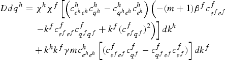 $$\eqalign{D dq^h & = \chi^{h}\chi^{f} \left[\left(c^h _{e^h e^h }c^h _{q^h } -c^h _{q^h e^h } c^h _{e^h } \right)\left(-\lpar m+1\rpar \beta^f c_{e^f e^f }^f \right.\right.\cr & \quad \left.\left. -k^f c^f _{e^f e^f }c^f _{q^f q^f }+ k^f \lpar c^f _{e^f q^f }\rpar ^{2} \right)\right]dk^h \cr &\quad + k^h k^f \gamma mc^h _{e^h e^h }\left[\lpar c^f _{e^f e^f }c^f _{q^f } -c^f _{q^f e^f }c^f _{e^f }\rpar \right]dk^f} $$
where D > 0 is the determinant of the coefficient matrix and
 $c^z_{e^z e^z} c^z_{q^z} -c^z_{q^z e^z} c^z_{e^z}\gt0$
for z = h, f.
$c^z_{e^z e^z} c^z_{q^z} -c^z_{q^z e^z} c^z_{e^z}\gt0$
for z = h, f.
Next, I shall derive the expression in (19) and (20). Let
 $E=E\lpar \breve{k^h }\comma \; \breve{k^f }\comma \; s^h \comma \; s^f {\comma \; \tau^h \comma \; \tau^f \rpar }$
and
$E=E\lpar \breve{k^h }\comma \; \breve{k^f }\comma \; s^h \comma \; s^f {\comma \; \tau^h \comma \; \tau^f \rpar }$
and
 $ \pi^h =\pi^h \left(\breve{q}^{h}\lpar{\cdot}\rpar \comma \; \breve{q}^{f}\lpar{\cdot}\rpar \comma \; \breve{k^h }\comma \; \breve{k^f }\comma \; s^h \comma \; s^f {\comma \; \tau^h \comma \; \tau^f }\right)$
,
$ \pi^h =\pi^h \left(\breve{q}^{h}\lpar{\cdot}\rpar \comma \; \breve{q}^{f}\lpar{\cdot}\rpar \comma \; \breve{k^h }\comma \; \breve{k^f }\comma \; s^h \comma \; s^f {\comma \; \tau^h \comma \; \tau^f }\right)$
,
 $\pi^f =\pi^f \left(\breve{q} ^{h}\lpar{\cdot}\rpar \comma \; \breve{q}^{f}\lpar{\cdot}\rpar \comma \; \breve{k^h }\comma \; \breve{k^f }\comma \; s^h \comma \; s^f {\comma \; \tau^h \comma \; \tau^f }\right)$
where
$\pi^f =\pi^f \left(\breve{q} ^{h}\lpar{\cdot}\rpar \comma \; \breve{q}^{f}\lpar{\cdot}\rpar \comma \; \breve{k^h }\comma \; \breve{k^f }\comma \; s^h \comma \; s^f {\comma \; \tau^h \comma \; \tau^f }\right)$
where
 $\breve{k^h }=\breve{k^h }\lpar s^h \comma \; s^f {\comma \; \tau^h \comma \; \tau^f \rpar }$
,
$\breve{k^h }=\breve{k^h }\lpar s^h \comma \; s^f {\comma \; \tau^h \comma \; \tau^f \rpar }$
,
 $\breve{k^f }=\breve{k^f }\lpar s^h \comma \; s^f {\comma \; \tau^h \comma \; \tau^f \rpar }$
,
$\breve{k^f }=\breve{k^f }\lpar s^h \comma \; s^f {\comma \; \tau^h \comma \; \tau^f \rpar }$
,
 $\breve{q}^{h}=\breve{q }^{h}\lpar \breve{k^h }\comma \; \breve{k^f }\comma \; s^h \comma \; s^f {\comma \; \tau^h \comma \; \tau^f \rpar }$
,
$\breve{q}^{h}=\breve{q }^{h}\lpar \breve{k^h }\comma \; \breve{k^f }\comma \; s^h \comma \; s^f {\comma \; \tau^h \comma \; \tau^f \rpar }$
,
 $\breve{q}^{f}= \breve{q}^{f}\lpar \breve{k^h }\comma \; \breve{k^f }\comma \; s^h \comma \; s^f {\comma \; \tau^h \comma \; \tau^f \rpar }$
. Using the first order conditions
$\breve{q}^{f}= \breve{q}^{f}\lpar \breve{k^h }\comma \; \breve{k^f }\comma \; s^h \comma \; s^f {\comma \; \tau^h \comma \; \tau^f \rpar }$
. Using the first order conditions
 $\pi^h _{\breve{q}^{h}}=0$
and
$\pi^h _{\breve{q}^{h}}=0$
and
 $\pi^h _{\breve{k^h }}=0$
, and the fact that
$\pi^h _{\breve{k^h }}=0$
, and the fact that
 $\pi^h _{\breve{k^f }}=0$
, the differentiation, of (18) yields the effects via the policy given in (19). Applying the results in (19) to the foreign country one obtains
$\pi^h _{\breve{k^f }}=0$
, the differentiation, of (18) yields the effects via the policy given in (19). Applying the results in (19) to the foreign country one obtains
 $$W_{s^f }^{f}=0\Rightarrow {m\pi^f_{q^h }\left(q^h _{k^f }k^f _{s^f }+q^h _{k^h } k^h _{s^f }+q^h _{s^f }\right)+m\pi^f_{s^f }\over \phi ^{f \prime }}=E_{s^f }+E_{k^h } k^h _{s^f }+E_{k^f }k^f _{s^f }.$$
Substituting (A.2) into W s f h and collecting terms gives (20).

