INTRODUCTION
Phytoplankton are an efficient and easily detectable indicator of ecological change and are of great importance for aquatic ecosystems, being sensitive to numerous environmental stressors (Paerl et al., Reference Paerl, Valdes-Weaver, Joyner and Winkelmann2007). Primary production is one of the most important ecological aspects of phytoplankton and the biomass built through photosynthesis is the nutritional basis for all higher trophic levels. Many phytoplankton species occur all year round, while others occur only in particular seasons (Hoppenrath et al., Reference Hoppenrath, Elbrächter and Drebes2009). Estuaries are transition zones between riverine and maritime environments, and they are known as highly productive ecosystems. Many studies on the phytoplankton community have been conducted in estuaries around the Mediterranean Sea, which are generally stratified in their middle and lower sections and well-mixed in the upper section (Trigueros & Orive, Reference Trigueros and Orive2001; Cetinić et al., Reference Cetinić, Viličić, Burić and Olujić2006; Burić et al., Reference Burić, Cetinić, Viličić, Mihalić, Carić and Olujić2007; Lopes et al., Reference Lopes, Lillebø, Dias, Pereira, Vale and Duarte2007; Barbosa et al., Reference Barbosa, Domingues and Galvão2010; Domingues et al., Reference Domingues, Barbosa, Sommer and Galvão2012).
Unplanned urbanization and increasing industrial facilities around the Golden Horn Estuary (GHE) since the 1950s have caused severe pollution, particularly due to pharmaceutical, detergent, dye and leather industries, and domestic wastewater discharge (Yüksek et al., Reference Yüksek, Okuş, Yilmaz, Aslan-Yilmaz and Taş2006). By the early 1990s, estuarine life was limited to the area around the Galata and Atatürk Bridges due to anoxia and heavy sedimentation. The Golden Horn Rehabilitation Project was initiated in 1997, in order to remove pollution and improve water quality. For this purpose, surface discharges were connected to collector systems, a high amount of anoxic sediment was removed from the almost completely filled upper section and the Valide Sultan Bridge, which floats on pontoons, was semi-opened to increase water circulation. These efforts resulted in rapid renewal and oxygenation of anoxic sediment and water mass, which was followed by increasing phytoplankton activity (Yüksek et al., Reference Yüksek, Okuş, Yilmaz, Aslan-Yilmaz and Taş2006).
Phytoplankton studies performed before the rehabilitation of the GHE showed that insufficient water circulation, extreme pollution caused by industrial and domestic wastewater discharges and low light availability limited phytoplankton growth and species diversity particularly in the upper estuary (Uysal & Unsal, Reference Uysal and Unsal1996; Tas & Okus, Reference Tas and Okus2003). Following rehabilitation, the changes in the ecosystem such as increasing water circulation, dissolved oxygen concentration and water transparency stimulated the growth and species richness of phytoplankton assemblages (Tas et al., Reference Tas, Yilmaz and Okus2009). In recent years, many studies have focused on algal blooms and potentially harmful microalgae (Tas, Reference Tas2015, Reference Tas2017; Tas & Yilmaz, Reference Tas and Yilmaz2015; Dursun et al., Reference Dursun, Taş and Koray2016; Tas & Lundholm, Reference Tas and Lundholm2016), toxic diatom species and their toxins (Tas et al., Reference Tas, Dursun, Aksu and Balkis2016; Dursun et al., Reference Dursun, Unlu, Tas and Yurdun2017), and planktonic diatom composition in the GHE (Tas, Reference Tas2017).
The aim of this study is to investigate the variations in abundance and diversity of the phytoplankton community in the GHE in relation to environmental variables. We hypothesized that the spatial and temporal distribution of the phytoplankton community in the surface waters of the GHE depends on the changing environmental conditions.
MATERIALS AND METHODS
Study area
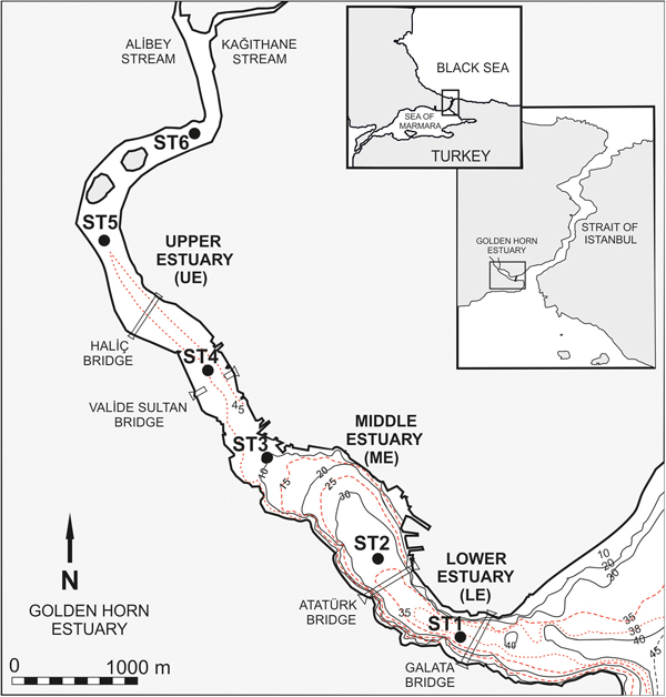
The Golden Horn Estuary (GHE) is located in the north-east of the Sea of Marmara, extending in a north-west–south-east direction, ~7.5 km long and 700 m wide, with a surface area of 2.6 km2 (Figure 1). The study area was categorized in three sections based on the hydrographic and bathymetric structure; lower estuary (LE), middle estuary (ME) and upper estuary (UE). The depth is 40 m in the LE, it decreases rapidly to 14 m in the ME, and to 4 m in the UE due to sedimentation (Figure 1). Six stations were distributed along the study area; ST1 represents the LE and interacts strongly with the Strait of Istanbul (Bosphorus). ST2 and ST3 represent the ME, where a bridge operating on buoys (Atatürk Bridge) limits upper layer circulation between the lower and upper estuaries. ST4, ST5 and ST6 are located in the UE, and influenced by two streams (Alibey and Kağıthane). The streams were the main sources of freshwater input before the construction of a series of dams at the end of the 1990s. Hence, the amount of freshwater inflow decreased considerably and nowadays, rainfall is the main source of fresh water flowing into the study area (Sur et al., Reference Sur, Okuş, Sarikaya, Altiok, Eroğlu and Öztürk2002). The LE is characterized by two-layered stratification: with the less saline (~18‰) Black Sea water above and the highly saline (~38‰) Mediterranean water below (Özsoy et al., Reference Özsoy, Oğuz, Latif, Ünlüata, Sur and Beşiktepe1988). The upper layer extends to depths of about 25 m and the lower layer lies below ~25 m. The interface between the two layers lies between 16 and 28 m (Sur et al., Reference Sur, Okuş, Sarikaya, Altiok, Eroğlu and Öztürk2002).

Fig. 1. Study area and sampling stations.
Sampling and seawater analyses
The sampling period covered one year, from August 2011 to July 2012. Seawater samples were collected at monthly (August to February, June to July) and biweekly (from March to May) intervals from six stations, representing the LE, ME and UE sections (Figure 1). Samples were taken from the surface (0.5 m) using 5 L Niskin bottles. Temperature, salinity, dissolved oxygen (DO) and pH were measured using a multi-parameter probe (YSI Professional Pro Plus), and a 30 cm diameter Secchi disc was used for water transparency. Samples for nutrient analysis were pre-filtered through 5 µm syringe filters and kept frozen at −20°C until they were analysed. Dissolved inorganic nutrients (NO3 + NO2, PO4 and SiO2) were determined using a Bran + Luebbe AA3 auto-analyser according to standard methods (APHA, 1999). Chlorophyll-a (Chl-a) analyses were carried out by applying the acetone extraction method (Parsons et al., Reference Parsons, Maita and Lalli1984). No phytoplankton data could be obtained from the UE in January probably due to very high concentrations of suspended particulate matter (SPM) at the surface.
Phytoplankton analysis
For enumeration and identification of phytoplankton, seawater samples were transferred into 250 ml glass bottles and preserved with acidic Lugol's solution (to a final concentration of 2%) (Throndsen, Reference Throndsen and Sournia1978). Subsamples (50, 25 or 10 mL) were settled in sedimentation chambers for 24–48 h (Utermöhl, Reference Utermöhl1958) and examined under an inverted microscope equipped with phase contrast (Leica DM IL LED) at 100 × or 200 × magnifications, because this study was aimed at micro-phytoplankton in particular (20–200 µm cell size). Cell counts were generally performed on two or more transects, counting at least 300 cells in each sample and phytoplankton abundance was calculated as cells per litre.
A total of 45 net samples were collected, to determine species richness in the phytoplankton community, using a Nansen plankton net (0.57 m diameter, 55 µm mesh size) by vertical tows from 10 m to the surface at ST1, ST2 and ST3. Net samples were transferred to jars and preserved with borax-buffered formaldehyde (to a final concentration of 4%). Species identification was performed under a light microscope equipped with a Leica DFC camera (Leica DM 2500) at 100× to 400× magnifications. All net samples were collected simultaneously with the bottle samples. No phytoplankton data could be obtained from the UE in January.
Data analysis
Principal component analyses (PCA) were used to explore the spatial and temporal variations in environmental parameters (temperature, salinity, Secchi depth, pH, DO, NO3 + NO2, PO4 and SiO2). Prior to all PCAs, environmental data were transformed to fourth root to reduce the heterogeneity in the data and to normalize the distribution using the Primer v6 program. The relationships between environmental parameters and total number of species (S), Shannon diversity index (H’), Chl-a, total phytoplankton abundance (N-Total), diatom abundance (N-Dia) and dinoflagellate abundance (N-Dino) were analysed by Spearman rank correlation following transformations to natural logarithms, using Statistica 6.0 software. Spatio-temporal patterns in physical, chemical and biological data were also investigated among sections of the estuary and months by one-way analysis of variance (ANOVA). Prior to ANOVA, all environmental data were normalized by logarithmic transformation using SPSS Statistics 21.0 software.
RESULTS
Physical variables
Generally, the UE had higher temperature values than the LE. Surface temperature varied from 4.1°C (February, LE) to 26.5°C (July, UE) (Figure 2). Mean annual temperature was 13.3 ± 6.3°C at the LE and 15.0 ± 7.4°C at the UE (Table 1). Salinity was relatively stable in the LE, but it was highly variable in the UE (Figure 2). In contrast to temperature, salinity values were always lower in the UE. Surface salinities varied between 9.8 (February, UE) and 19.9 (September, LE). Mean annual salinity was 19.0 ± 0.49 in the LE and 16.4 ± 2.65 in the UE (Table 1). Water transparency based on Secchi disc depth, decreased markedly from the LE to the UE. The lowest Secchi disc depths were measured in the UE, probably due to the high amount of SPM carried by the two streams. Minimum Secchi depth was 0.6 m in the UE (May), whereas its maximum value was 10 m in the LE (December) (Figure 2). Mean annual Secchi depth was 6.4 ± 2.1 m in the LE and 1.3 ± 0.6 m in the UE (Table 1). Temperature showed a seasonal pattern, while salinity and Secchi depth displayed significant variations among the sections of the estuary (Table 2).

Fig. 2. Temporal fluctuations in environmental variables in the GHE.
Table 1. The mean values and standard deviations (Mean ± SD), minimum and maximum values of environmental variables in surface water of three sections of the GHE during the study period.

Table 2. Significant one-way analysis of variance (ANOVA) results of spatiotemporal patterns in environmental data.

Chemical variables
In general, nutrient concentrations increased over the winter months and decreased in late spring and during summer (Figure 2). Nutrient values were more stable in the LE, while they were highly variable in the UE. Surface nutrient values, with the exception of NO3 + NO2, increased gradually from the LE to the UE (Figure 2). NO3 + NO2 concentrations ranged between 0.04 and 25.6 µM, with a mean value of 3.5 ± 3.4 µM for the LE and 7.3 ± 7.3 µM for the UE (Table 1), and decreased significantly after the beginning of spring. PO4 concentrations varied between 0.1 and 10.8 µM, with a mean value of 0.46 ± 0.36 for the LE and 3.01 ± 2.9 µM for the UE (Table 1), while the highest values were measured in early summer. SiO2 concentrations ranged between 1.8 and 20.1 µM, with a mean value of 8.3 ± 3.7 µM for the LE and 12.0 ± 6.8 µM for the UE (Table 1), and were relatively high between December and April (Figure 2). PO4 concentrations displayed a spatial pattern, while NO3 + NO2 and SiO2 concentrations displayed a significant seasonal pattern (Table 2).
DO concentrations were generally higher in the LE and decreased from the LE to the UE. Surface DO concentrations ranged between 0.2 mg L−1 (UE, May) and 16.9 mg L−1 (LE, January) (Figure 2). Mean annual DO concentrations varied between 11.8 ± 2.70 mg L−1 in the LE and 4.67 ± 2.74 mg L−1 in the UE (Table 1). pH values were relatively high between September and January, and surface values varied between 7.02 (LE, August) and 9.08 (ME, December), while showing a decreasing trend over the sampling period (Figure 2). Mean annual pH values were 7.94 ± 0.53 and 8.13 ± 0.32 in the LE and UE, respectively (Table 1). Chl-a concentrations ranged between 0.6 and 3.7 in the LE, 0.7 and 86.0 in the ME, 0.8 and 26.8 µg L−1 in the UE. Chl-a values increased considerably in spring and reached the highest level (86.0 µg L−1, May) in the ME (Figure 2). Mean annual Chl-a values varied between 1.73 ± 0.87 and 7.57 ± 8.07 µg L−1 from the LE to the UE, while the highest mean value was 9.68 ± 21.5 µg L−1 in the ME (Table 1). DO concentrations displayed a spatial pattern, while pH displayed a seasonal pattern (Table 2).
Species composition and diversity
A total of 78 phytoplankton taxa belonging to eight algal classes were identified in bottle and net samples (180 bottle and 45 net samples) collected during the study period. Sixty-seven taxa were identified to species level and 11 taxa to genera. Among these, 38 taxa (48.7%) were diatoms, 30 taxa (38.5%) were dinoflagellates and 10 taxa (12.8%) were phytoflagellates, including silicoflagellates, cryptophycean, raphidophycean, crysophycean, euglenophyceans and chlorophyceans. Eight taxa were observed only in net samples. The number of diatoms and dinoflagellates, the major groups, accounted for 87.2% of the total phytoplankton species identified during this study. The most diverse genera were the diatoms Chaetoceros and Rhizosolenia, and the dinoflagellates Protoperidinium and Tripos. The most frequent and abundant species observed during the study period were the diatoms Pseudo-nitzschia spp., Skeletonema marinoi, Thalassiosira sp.; the dinoflagellates Tripos furca, T. fusus; and the phytoflagellates Plagioselmis prolonga and Heterosigma akashiwo.
The highest number of species (S) was found in the lower and middle estuary and decreased markedly in the upper estuary (Figures 3 & 4). The average S was 8.7 in the lower estuary, while it was 6.0 in the middle estuary and only 2.8 in the upper estuary, obtained from bottle samples during the study period. The results showed that S was generally high in autumn and winter, while it was low in spring. Diatoms were more diverse in summer and autumn, while dinoflagellates were richer in spring (Figure 3). Group composition based on species diversity indicated that the number of diatom and dinoflagellate species was higher in the lower estuary and they decreased towards the upper estuary, while phytoflagellates were more frequent in the upper estuary (Figure 3). Variations in S were well-correlated with the increase in salinity, Secchi depth and DO and the decrease in nutrient values at all stations (Table 3).

Fig. 3. Spatio-temporal variations in the number of species in each phytoplankton group during the study period.

Fig. 4. Spatio-temporal variations in the total number of species and Shannon diversity index.
Table 3. Spearman rank correlation coefficients (rho) between environmental variables and total number of species (S), Shannon diversity index (H′), total phytoplankton abundance (N-Total), diatom abundance (N-Dia), dinoflagellate abundance (N-Dino) and Chl-a.

Statistically significant correlations are indicated by symbols: – not significant; *P < 0.05; **P < 0.01.
The Shannon diversity index (H ′) fluctuated significantly between the lower and upper estuary. The fluctuations of H ′ were generally in line with species number (S) (Figure 4). Higher diversity was mostly detected in the lower estuary. The highest and average H ′ was measured between 3.00 and 1.74 in the LE, 3.06 and 1.34 in the ME, 1.54 and 0.44 in the UE, indicating a clear decline in diversity from the lower to the upper estuary. The values of H ′ were correlated with the increase in salinity, Secchi depth and DO and the decrease in nutrient values at all stations, as in the case of S mentioned above (Table 3).
Abundance patterns
Total phytoplankton abundance (N) showed seasonal and spatial fluctuations, increasing in spring and summer, particularly in the middle and upper estuary. N was relatively low in winter, while it began to increase in March and remained high until August. Higher abundances in phytoplankton were detected in the middle and upper estuary except in March. The highest phytoplankton abundance reached 10,429 × 103 cells L−1 in the UE in late May (Figure 5). There was a positive correlation between N and temperature (P < 0.05) only in the UE and a negative correlation between N and SiO2 at all stations, probably due to diatom Si-uptake (Table 3).

Fig. 5. Spatio-temporal variations in phytoplankton abundance during the study period.
Group composition in terms of cell abundance varied among the sections of the estuary. Diatoms were clearly more abundant in the lower and middle estuary, while dinoflagellates and phytoflagellates were more abundant in the upper estuary (Figure 5). The average contribution of diatom species to total phytoplankton abundance decreased considerably from the LE to the UE (from 79% to 40%), while the average contribution of flagellate groups increased markedly from the LE to the UE (from 21% to 60%) (Figure 6).

Fig. 6. Percentage of the abundance of main groups in total phytoplankton community during the study period.
Diatom abundance displayed a slightly seasonal difference among the sections of the estuary. In the lower estuary, diatoms were relatively more abundant in spring, while they were more abundant in the middle and upper estuary in summer (Figures 5 & 6). Highest diatom abundance reached 1971 × 103 cells L−1, dominated by Skeletonema marinoi in the LE in March (Figure 5). Skeletonema marinoi formed a spring bloom in the lower estuary with maximum abundance of 1950 × 103 cells L−1 (Figure 7). Another diatom increase was observed in the upper estuary in August caused by Thalassiosira sp., with maximum abundance of 1560 × 103 cells L−1. Thalassiosira sp. was not a common species and, in general, was observed between August and October during the study period (Figure 7). Other common diatom species were Pseudo-nitzschia species in the study area with a maximum abundance of 210 × 103 cells L−1 in the lower estuary in May (Figure 7). Diatom abundance was negatively correlated with PO4 and SiO2 (P < 0.01) at all stations, indicating nutrient uptake. In addition, there was a weak positive correlation between diatom abundance and Secchi depth/DO (P < 0.05) among all stations (Table 3).

Fig. 7. Spatio-temporal variations in some important phytoplankton species.
Dinoflagellate abundance was generally lower compared with that of the other groups during the study period, and higher abundances were found in the middle and upper estuary in particular. Highest dinoflagellate abundance reached 459 × 103 cells L−1, dominated by Scrippsiella trochoidea in the UE in July. The same species reached 131 × 103 cells L−1 in June, as well. Scrippsiella trochoidea was detected only in summer in the study area (Figure 7). The other most abundant dinoflagellate was Prorocentrum triestinum and its abundance reached 84 × 103 cells L−1 in the ME in August. Another common dinoflagellate species was Prorocentrum micans and its abundance reached 25 × 103 cells L−1 in the ME in November (Figure 7). The most common dinoflagellate species in the study area were Tripos furca and T. fusus. These species were more abundant in autumn and winter generally, with abundances of <3 × 10³ cells L−1 except in November (T. fusus, 6.2 × 10³ cells L−1) (Figure 7). Dinoflagellate abundance was well-correlated with salinity, Secchi depth, DO, NO3 + NO2 and SiO2 among all stations. The effect of temperature on dinoflagellate abundance was only seen in the UE (Table 3).
Plagioselmis prolonga, Heterosigma akashiwo and some euglenophyceans were common and abundant in the GHE during the study period. Plagioselmis prolonga, a bloom-forming cryptophycean, was observed only in November and May and its maximum abundance reached 1040 × 103 cells L−1 in the upper estuary in May (Figure 7). Another bloom-forming species was the raphidophycean Heterosigma akashiwo that was commonly observed between February and May. A dense bloom of H. akashiwo occurred in the upper estuary in late May with a rapid temperature rise and maximum abundance reached 10,400 × 103 cells L−1 (Figure 7). Euglenophyceans including euglenoids and Eutreptiella sp. were frequently observed in the study area particularly between April and July. The highest abundance of euglenophyceans was 132 × 103 cells L−1 in the upper estuary in June (Figure 7).
Data analysis
PCA analyses showed a significant spatial variation in environmental variables during the study period (Figure 8A). The first two PCs explained 79.7% of the cumulative variation (PC1: 53.4%, PC2: 26.3%). Projection of sections on the PCA ordination reflected a significant separation of stations from the LE to the UE in the ordination plane along a horizontal transect (Figure 8A). This indicated the highest variation in the UE and the lowest variation in the LE. Projection of sampling months on the PCA ordination showed a seasonal variation in the ordination plane along a diagonal transect (Figure 8B). Coefficients in the linear combinations of variables making up PCs showed that nutrients (DIN and silicate), temperature, Secchi depth and DO are the most important on the PC1 (Figure 8A), while Secchi depth, DO, DIP, DIN and temperature are the most important on the PC2 (Figure 8B). pH and salinity do not influence the ordination, probably due to low number of samples and long intervals of sampling. Higher concentration of DIN and silicate characterized the winter samples mainly in the UE, due to weak phytoplankton uptake and high terrestrial input by streams, whilst ME and LE show lower concentration. Thus, the results of PCAs show that the main environmental factors (nutrients, temperature, Secchi depth) cause the spatial and temporal variation of phytoplankton in the study area.

Fig. 8. PCA ordination of environmental variables at sections of the GHE (A) and sampling months (B).
DISCUSSION
Eutrophication in estuarine and coastal marine ecosystems significantly increases phytoplankton biomass (Smith et al., Reference Smith, Tilman and Nekola1999). The effects of eutrophication on the GHE ecosystem have been seen in dense algal blooms (Tas et al., Reference Tas, Yilmaz and Okus2009; Tas & Okuş, Reference Tas and Okuş2011; Tas, Reference Tas2015; Tas & Yilmaz, Reference Tas and Yilmaz2015). As in previous studies, this study showed that eutrophication in the GHE increases phytoplankton abundance particularly in spring and summer.
Phytoplankton studies performed in Mediterranean Sea estuaries indicate that environmental forcing factors such as temperature, salinity, water transparency and nutrients play an important role in the seasonal variation of phytoplankton, both in terms of abundance and diversity (Cetinić et al., Reference Cetinić, Viličić, Burić and Olujić2006; Burić et al., Reference Burić, Cetinić, Viličić, Mihalić, Carić and Olujić2007; Barbosa et al., Reference Barbosa, Domingues and Galvão2010; Jasprica et al., Reference Jasprica, Carić, Kršinić, Kapetanović, Batistić and Njire2012). The present study indicated that light availability and highly variable salinity limit the growth of phytoplankton particularly in the upper estuary, as reported by the previous studies (Cloern, Reference Cloern1987, Reference Cloern1999; Mallin et al., Reference Mallin, Cahoon, McIver, Parsons and Christopher Shank1999). Light limitation affects the growth of phytoplankton in the upper section of the GHE as stated in previous studies (Uysal, Reference Uysal1987; Tas & Okus, Reference Tas and Okus2003; Tas et al., Reference Tas, Yilmaz and Okus2009, Reference Tas, Dursun, Aksu and Balkis2016) and is the most important factor explaining the lack of phytoplankton, particularly in the upper estuary in January, and is related to the high SPM that is probably due to increasing terrestrial inputs during rainy periods.
The increase of nutrient inputs may result in a shift in phytoplankton composition (Domingues et al., Reference Domingues, Barbosa, Sommer and Galvão2011), as well as in changes to the seasonal succession of phytoplankton assemblages (Lopes et al., Reference Lopes, Lillebø, Dias, Pereira, Vale and Duarte2007). Light and nutrient availability are generally controlled by river flow (Domingues et al., Reference Domingues, Barbosa, Sommer and Galvão2012). These results are generally consistent with the present study. Burić et al. (Reference Burić, Cetinić, Viličić, Mihalić, Carić and Olujić2007) suggested that nutrients strongly limit phytoplankton growth in summer when river discharge is minimal. Our study revealed that nutrients may limit phytoplankton growth only in the lower estuary during summer.
The number of phytoplankton taxa recorded during our study period was lower than that of the earlier studies carried out in the GHE (Tas et al., Reference Tas, Yilmaz and Okus2009; Tas & Yilmaz, Reference Tas and Yilmaz2015). In a study performed between 1998 and 2002, 142 phytoplankton taxa were identified in all samples (Tas et al., Reference Tas, Yilmaz and Okus2009). In another study, with more frequent sampling, performed between 2009 and 2010, 155 phytoplankton taxa were identified in all samples (Tas & Yilmaz, Reference Tas and Yilmaz2015). The dissimilarity in the number of species between different years might be due to the frequency and number of sampling periods, and also the study time period. The contribution of diatom and dinoflagellate species to the number of total phytoplankton was relatively lower (87.2%), while that of phytoflagellates was higher (12.8%), when compared with earlier studies (Tas et al., Reference Tas, Yilmaz and Okus2009; Tas & Yilmaz, Reference Tas and Yilmaz2015). This situation may be explained by the differences in the total number of samples collected during the study period and sampling frequencies. However, group composition of phytoplankton and most abundant species were generally consistent with the study performed by Jasprica et al. (Reference Jasprica, Carić, Kršinić, Kapetanović, Batistić and Njire2012) in the lower Neretva River estuary (Eastern Adriatic Sea). Jasprica et al. (Reference Jasprica, Carić, Kršinić, Kapetanović, Batistić and Njire2012) suggested that diatoms and dinoflagellates were the major groups (88.5%) representing the phytoplankton community, while the remaining groups were mostly nanoplanktonic species, as mentioned above for this study. Furthermore, the abundant species were the diatoms Skeletonema marinoi and Thalassiosira sp.; and the dinoflagellate Scrippsiella trochoidea, as reported by Jasprica et al. (Reference Jasprica, Carić, Kršinić, Kapetanović, Batistić and Njire2012).
Burić et al. (Reference Burić, Cetinić, Viličić, Mihalić, Carić and Olujić2007) suggested that diatoms dominated in early spring, while dinoflagellates and nano-phytoplankton dominated in summer, in a highly stratified estuary (Zrmanja, Adriatic Sea). In this study, however, diatoms dominated the phytoplankton community in early spring in the lower estuary, and in late summer in the middle and upper estuary, while dinoflagellates and nanoplanktonic phytoflagellates dominated the phytoplankton community in the upper estuary. This indicates that algal groups in the GHE may change quickly depending on environmental conditions. More stable conditions in the lower and middle estuary than those in the upper estuary provided more suitable conditions for the growth of diatoms, whereas unstable conditions (low water transparency, highly variable salinity) in the upper estuary favoured nanoplanktonic phytoflagellates, as stated by Burić et al. (Reference Burić, Cetinić, Viličić, Mihalić, Carić and Olujić2007). As is well-known, environments with high nutrient levels stimulate the growth of the euglenophycean Eutreptiella gymnastica (Olli et al., Reference Olli, Heiskanen and Seppälä1996). High organic and inorganic nutrient load in the upper estuary may favour the growth and blooms of euglenophyceans.
The decrease in the number of species in the UE is due to poor water quality, including very low water transparency, sometimes very low DO, high amounts of nutrients and inadequate water circulation. Thus, these may be considered the most important factors influencing the number of species in the UE. These results agree with the earlier studies (Tas et al., Reference Tas, Yilmaz and Okus2009; Tas, Reference Tas2017). In general, diatom abundance was negatively correlated with DO in the upper estuary, because local conditions limit the growth of diatoms, however the positive correlation between diatoms and DO indicates the high abundance of diatoms in May.
The abundance pattern displayed spatial and temporal fluctuations in the GHE that are similar to those of previous studies (Tas et al., Reference Tas, Yilmaz and Okus2009; Tas & Yilmaz, Reference Tas and Yilmaz2015). Increasing abundance in spring indicates suitable conditions for the growth of phytoplankton (e.g. rising temperature and water transparency) in the study area. Variations in group composition are important for assessing the available conditions. The contribution of diatoms to total phytoplankton abundance decreased considerably in the upper estuary due to poor water quality as mentioned above. The contribution of dinoflagellates and phytoflagellates to total phytoplankton abundance was higher in the middle and upper estuary. The different feeding modes in these groups may help them to compete with other species for growth under local conditions. Variations in group composition in the study area are compatible with other studies (Tas et al., Reference Tas, Yilmaz and Okus2009; Tas & Lundholm, Reference Tas and Lundholm2016; Tas, Reference Tas2017).
Algal blooms in the GHE have been discussed in detail by several studies (Tas et al., Reference Tas, Okuş and Aslan-Yılmaz2006, Reference Tas, Yilmaz and Okus2009; Tas & Okuş, Reference Tas and Okuş2011; Tas, Reference Tas2015; Tas & Yilmaz, Reference Tas and Yilmaz2015; Dursun et al., Reference Dursun, Taş and Koray2016; Tas & Lundholm, Reference Tas and Lundholm2016). Dense algal blooms, except for the raphidophycean Heterosigma akashiwo, were not recorded in the GHE during the study period. The first dense bloom of H. akashiwo caused water discolouration in the GHE (Tas & Yilmaz, Reference Tas and Yilmaz2015). During this study, the bloom of H. akashiwo occurred in the UE almost at the same time as that of the previous study. Results indicated that a rapid temperature rise in spring was the most important factor that caused a bloom of H. akashiwo, as reported by Dursun et al. (Reference Dursun, Taş and Koray2016). Nevertheless, high abundances were detected for diatoms Skeletonema marinoi and Thalassiosira sp., and the cryptophycean Plagioselmis prolonga, which are known to be bloom-forming species for the GHE (Tas et al., Reference Tas, Yilmaz and Okus2009; Tas & Yilmaz, Reference Tas and Yilmaz2015).
In conclusion, the results obtained by this study revealed that phytoplankton composition and abundance vary among the sections of the estuary and at different seasons depending on the changing environmental conditions. Regular monitoring studies would be very useful for gaining a better understanding of the changes in the GHE ecosystem, which is a potential risk area for future harmful algal blooms.
ACKNOWLEDGEMENTS
The authors wish to thank Dr Ahsen Yüksek and Dr Muharrem Balcı for assistance with nutrient analysis. We are also grateful to Dr Selma Ünlü, technicians Özkan Çamurcu, Sezgin Çamurcu and Adem Okuş for their contribution in field and laboratory studies.
FINANCIAL SUPPORT
This work was supported by the Scientific Research Projects Coordination Unit of Istanbul University. Project number: 18585.