


NOMENCLATURE
- b
-
aerofoil model breadth (=750 mm)
- cp
-
pressure coefficient
- c (ref)
-
aerofoil (reference) chord (=160 mm)
- CL
-
global lift coefficient
- Cl
-
local lift coefficient
- CM
-
global aerodynamic moment coefficient
- Cm
-
local aerodynamic moment coefficient
- D
-
damping matrix
- F
-
force [N]
- f
-
frequency [Hz]
- FoS
-
factor of safety
- f a
-
aerodynamic force vector
- f s
-
structural force vector
- H
-
interpolation matrix
- k
-
reduced frequency: k = 2πfcref/u ∞
- K
-
stiffness matrix
- L
-
lift [N]
- M
-
mass matrix
- M
-
moment [Nm]
- Ma
-
Mach number
- p 0
-
total pressure [bar]
- r
-
radial position [mm]
- Re
-
Reynolds number
- T 0
-
total temperature [K]
- u ∞
-
free stream velocity [m/s]
- u
-
deformation vector
- ↗
-
upstroke
Greek Symbol
- α,
 $\overline{\alpha }$
-
angle-of-attack, mean angle [°]
- α±
-
sinusoidal motion amplitude [°]
- α span
-
span-wise angle-of-attack [°]
- ω
-
natural frequency
- ω2 k
-
kth eigenvalue
- Ω
-
generalised stiffness matrix

1.0 INTRODUCTION
In fast forward flight or highly loaded manoeuvring flight, dynamic stall leads to high negative pitching moments on the retreating blade of a helicopter. Thus, high pitch link and vibratory loads occur which can limit the flight envelope. The retreating blade experiences low relative flow velocities in comparison to the advancing blade; therefore, high angles of attack are required to realise lateral trim. The angle-of-attack varies sinusoidally over one full revolution.
The aerodynamics of a rotor blade in its once-per-revolution (1/rev) motion has been studied by means of pitching aerofoils for some time(Reference Liiva1,Reference Gardner, Richter, Mai, Altmikus, Klein and Rohardt2) . Although neglecting rotational effects and assuming uniform inflow conditions, these investigations help to understand dynamic stall and its dependence on Mach number, Reynolds number, mean angle-of-attack, pitching angle and frequency. During pitch oscillations, the onset of stall is delayed to higher angles of attack than in the static case. On the upstroke, large pressure gradients lead to boundary layer separation, vortices start to develop and travel from the leading to the trailing edge. High pitching moments occur when the main vortex passes over the blade. Experiments and simulations of oscillating wing tips(Reference Le Pape, Pailhas, David and Deluc3,Reference Merz, Wolf, Richter, Kaufmann and Raffel4) and rotating configurations(Reference McCroskey and Fisher5,Reference Mulleners, Kindler and Raffel6) have shown similar dynamic stall phenomena to the 2D cases.
Advanced blade tip planforms have the potential to improve retreating blade stall characteristics. Furthermore, blade vortex interactions and shock strength on the advancing blade can be reduced(Reference Schultz, Splettstoesser, Junker, Wagner, Schoell, Mercker, Pengel, Arnaud and Fertis7,Reference Rauch, Gervais, Cranga, Baud, Hirsch, Walter and Beaumier8) . Consequently, the performance and the flight envelope can be increased and noise and vibrations reduced. Investigations have sometimes been contradictory(Reference Scott, Sigl and Strawn9,Reference Yeager, Noonan, Singleton, Wilbur and Mirick10) , and no single best blade tip has yet emerged(Reference Brocklehurst and Barakos11). This uncertainty is not only due to different demands but also because of the complexity of the flow and the large number of parameters which have to be taken into account(Reference Mullins, Smith, Rath and Thomas12).
The double-swept model rotor blade tip ‘Möwe’ is investigated on an oscillation rig(Reference Wiggen and Voss13) in the Transonic Wind-Tunnel Göttingen (DNW-TWG) to offer new insights into 3D dynamic stall on a complex configuration (see Fig. 1). The patent of AIRBUS Helicopters ‘Noise and performance improved rotor blade for a helicopter’(Reference Schimke, Link and Schneider14), and the aerofoils, EDI-M112 and EDI-M109(Reference Gardner, Richter, Mai, Altmikus, Klein and Rohardt2), are taken as basis for the design of the wind-tunnel model. The experiment is designed to investigate the interaction of the dynamic stall vortices and the tip vortex on a double-swept rotor tip. The influences of reduced frequency, mean angle-of-attack and amplitude are examined. The model is designed to be as stiff as possible in order to reduce aeroelastic effects. However, the deformation of the model is measured in order to evaluate its influence on the aerodynamics. Besides the investigation of the flow phenomena described above, a validated numerical set-up has been established using the experimental data.
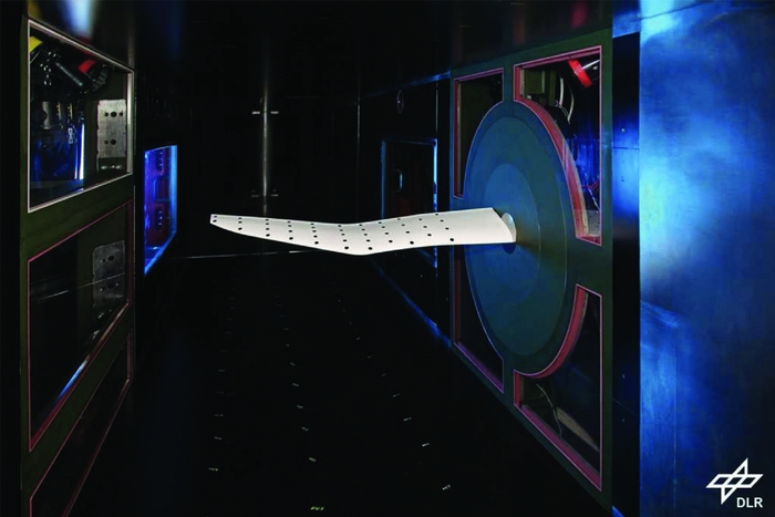
Figure 1. Pitching helicopter blade tip in the DNW-TWG.
This paper highlights how high-fidelity structural and aerodynamic simulations can be used to design the wind-tunnel experiment described above at the safety limit. The wind-tunnel facility and the chosen geometry are described in detail. Important structural design features and the finite element modelling of the carbon fibre model including results of the modal and the static analyses are shown. The finite element model is validated by an experimental modal analysis. Steady and unsteady RANS simulations are studied and validated with the experimental data from discrete pressure transducers. Expected and occurring flow phenomena and deviations between numerical and experimental data are discussed in detail.
2.0 EXPERIMENTAL SET-UP – BLADE-TIP GEOMETRY
The test section of the DNW-TWG, shown in Fig. 1, has a cross section of 1 m × 1 m. The lower and upper wall can be adapted to steady flow conditions by changing the wall shape to follow a streamline. Optical windows in the wind-tunnel sidewalls offer access for optical measurement systems. Flow phenomena are resolved by 60 unsteady pressure transducers (see Fig. 2), pressure sensitive paint and a piezoelectric balance(Reference Schewe15). Aeroelastic measurements are performed by two acceleration sensors and a 3D marker tracking system to record deformation. In this paper, only the experimental data of the pressure transducers are presented. Additional aerodynamic and thermodynamic parameters concerning the experimental set-up are listed in Table 1.
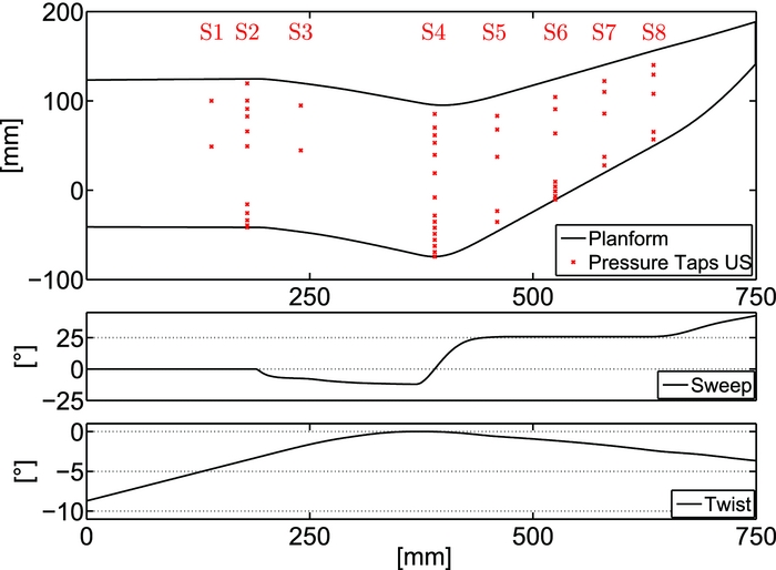
Figure 2. Planform of the model; location of the upper pressure taps; sweep and twist distribution.
Table 1 Geometric and aerodynamic boundary conditions of the experiment
A maximum model span of b = 750 mm was chosen in order to minimise the wind-tunnel wall interference on the blade tip. A high aspect ratio of 4.7 was chosen to include the point of first separation on a real rotor blade, which appears at a radial position of approximately 70%-90%. The planform, shown in Fig. 2, is derived from the parameterised patent of AIRBUS-Helicopters(Reference Schimke, Link and Schneider14): a rectangular section at the root, a forward swept section, a tapered backward swept section, and a parabolic shape for the outside section. The backward sweep is used to relieve the effects of compressibility at the advancing blade in forward flight. The forward sweep helps to move the centre of gravity forward and keeps the aerodynamic centre near the quarter-chord feathering axis of the blade. Thus, pitch link loads and vibrations can be reduced(Reference Brocklehurst and Barakos11). The pitch axis is positioned at the quarter-chord of the root section. The axis is flush with the wind-tunnel wall and a distance of 1.5 mm between wind-tunnel wall and root aerofoil ensures contactless operation.
The EDI-M112 aerofoil with 12% thickness is used for the inner unswept part of the blade since it shows soft trailing edge stall at low Mach number (Ma = 0.3–0.4)(Reference Gardner, Richter, Mai, Altmikus, Klein and Rohardt2). The EDI-M109 aerofoil with 9% thickness is used for the forward/backward swept part of the blade where higher Mach numbers occur. Along with the tapered outer part, a low drag coefficient is expected.
The twist angle of helicopter rotor blades usually decreases gradually from the root to the tip. In case of the pitching wind-tunnel model, the twist is decreased at the root in order to avoid dynamic stall being triggered by the separation at the wind-tunnel wall. Thus, the position of inner dynamic stall moves to a radial position of r ≈ 250 mm, where forward sweep begins. Here the sectional lift is at its maximum, while the interference of the wind-tunnel wall is negligible. For this model, the angle-of-attack refers to the angle of the chord at zero twist (r = 0.39 m) to the direction of the inflow. The blade tip has no anhedral, to reduce measurement complexity. The chord is nearly constant, c = 165 mm (small variations at the notch), until r = 400 mm. At the tip, the chord is c = 100 mm. The trailing edge is slightly modified at the tapered part to maintain a thickness of at least tTE = 0.5 mm. The small chord length and the thin aerofoils considerably limit the mounting space for pressure transducers and acceleration sensors.
3.0 CARBON FIBRE MODEL
The pitching wind-tunnel model is designed as a carbon fibre model because high bending and torsional stiffness, low weight, and sufficient mounting space for instrumentation are required. A high mass moment of inertia around the pitching axis and a strong bending-torsion coupling due to the planform is expected(Reference Rauch, Gervais, Cranga, Baud, Hirsch, Walter and Beaumier8). For stability reasons, a specific bending-torsion coupling to reduce the positive elastic twist is a further design goal. Since no centrifugal stiffening effects as under real flight conditions occur in the experiment, a high bending stiffness is a second design goal.
Thus, the wind-tunnel model is built up of an upper and a lower carbon composite shell (Table 2) which are bonded to a shaft and a spar (Fig. 3). At the leading edge, the upper and lower shell are connected by a leading-edge support structure.
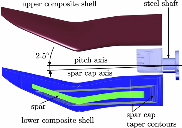
Figure 3. Catia V5 model of the rotor blade tip.
Table 2 Laminate of outer shells with M46J plies
The upper and lower shells are built using the unidirectional lamina M46J. A fibre volume fraction of ρ f ≈ 50% can be obtained by the hand lay-up method. Integrated unidirectional spar caps run from the steel shaft in the span-wise direction, tapering out at the beginning of the backward sweep (Fig. 3). Their fibres, which carry the main bending loads, are orientated forward at an angle of 2.5°. Thus, positive elastic twist is reduced in case of positive bending. The overlap of the unidirectional layers on the steel shaft is tapered 26:1 in span-wise direction and 8:1 in chord direction in order to reduce stress concentrations(Reference Bailie, Ley and Pasricha16). The spar consists of a foam core covered with ± 45° weave Style469. It experiences shear forces as a result of the lift, torsional loads as a result from the aerodynamic moments, and forced pitching inertial moments. The leading-edge bonding is a support structure of 0.8-mm-thick laminate Style469 ( ± 45°). Bonded to the composite shells and to the spar, a steel shaft (Fig. 4) transfers the loads to the Piezo balance which is interconnected between the model shaft and the hydraulic oscillation rig.
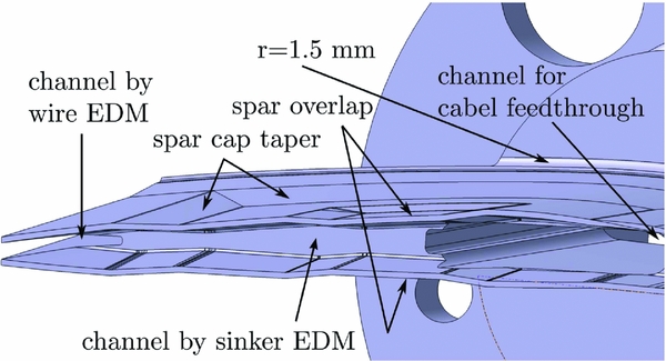
Figure 4. 42CrMo4 steel shaft with tapered channels.
The steel shaft has a corner radius of r = 1.5 mm in order to avoid high stress concentrations. A tapered channel is manufactured using sinker Electrical Discharge Machining (EDM) at the span-wise end of the steel shaft. Thus, a more homogeneous stress distribution in the laminate and the steel is obtained. Another tapered channel is manufactured using wire-cut EDM at the chord-wise end of the steel shaft for the same reason. Two overlapping regions between steel shaft and spar allow torsional load transfer between spar and root. A tapering of about 12:1 in span-wise and chord direction is provided for the overlapping weave of the spar. The shaft is hollow in order to integrate the cables and pressure reference tubes of the unsteady pressure tabs and the cables of the acceleration sensors. After the instrumentation of both shells, they are bonded together.
4.0 FINITE ELEMENT MODELLING
In order to detect local stress concentrations and weak spots, high-fidelity Finite Element (FE) models have been established by means of ANSYS(17). Shell elements are used for the laminate. Solid elements are used for the spar, bonding and shaft. The applied shell element SHELL281 is described by the first-order shear-deformation theory (Mindlin-Reissner). It has eight nodes with three translational and three rotational degrees of freedom at each node. The applied solid element SOLID186 is defined by 20 nodes having three translational degrees of freedom at each node. All material properties and deformations are considered linear. The shell elements are placed on the outer contour of the model because their thickness is not known in advance. Since the contour of the steel shaft depends on the final thickness of the laminate, an estimation of its thickness is required at the beginning. Based on existing wind-tunnel models, laminate thicknesses of t = 1.8 mm in the unreinforced region and t = 3.0 mm in the region of the integrated spar caps are chosen. Thus, the 2D shell elements of the outer composite surface and the 3D solid elements of the steel shaft have to be connected over a distance of the presumed thickness of the laminate. The same holds for the connection ‘outer surface – spar’ as well as for the connection ‘outer surface – leading-edge support structure’. In reality, the bonding procedure leads to an adhesive thickness of t ≈ 0.3 − 0.4 mm between the inner components and the outer contour. Two different modelling approaches (V1 and V2) for the connection of the outer contour to the shaft and the spar are proposed in the following (see Table 3).
In the model V1, which is shown in Fig. 5, the gap between inner components and outer contour is filled with solid elements with the material properties of epoxy. This kind of modelling is easy to accomplish, but leads to an adhesion thickness which is up to 10 times too thick.
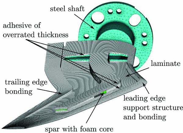
Figure 5. FE model V1 with solid elements for the connection ‘outer contour - shaft/spar’.
In the second, more sophisticated modelling approach V2, solid elements of t = 0.3 − 0.4 mm total thickness with the material properties of epoxy are implemented on the shaft (Fig. 6). The nodes of the free surface of the adhesive elements are connected by rigid links (CERIG) with the nodes of the shell elements on the outer contour. The steel shaft of V2 is adapted to the final contour and has small design changes in comparison to V1.

Figure 6. FE model V2; shaft and leading-edge bonding (rigid links are not displayed).
In both modelling approaches, the foam core of the spar is modelled with solid elements. The outer faces of the core volume are covered with shell elements simulating the ± 45° weave of t = 0.6 mm thickness. In version V1, the elements simulating the ± 45° weave are connected to the shell elements of the outer surface by 3D solid elements with epoxy properties. Again, this leads to an overestimated bonding thickness. In version V2 (Fig. 7), solid elements with the material properties of epoxy simulate a bonding of t = 0.4 mm thickness. The elements are modelled parallel to the upper and lower surface of the core. The upper and lower surface nodes of the spar are connected by rigid links with the opposite nodes of the solid elements, which represent the adhesive. The first approximation of the weave thickness t = 1.5 mm in V1 is reduced to t = 0.6 mm in V2, see Fig. 7. The nodes of the shell elements on the outer contour are connected by rigid links to the opposite nodes of the epoxy volume. This is only possible if the connected surfaces have the same node distribution. In model V1, holes for cable feed-through are integrated in the spar. The holes are eliminated for V2 because they lead to a significant weakening of the structure(see Section 6).
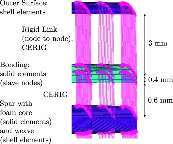
Figure 7. Spar, adhesive and outer surface connected via rigid links (V2).
For both model versions, the support structure of the leading-edge bonding is connected to the outer contour by solid elements with epoxy properties (Fig. 6). The adhesive of the leading-edge bonding is about ten times thinner in reality than in the model.
The axis of the hydraulic test oscillation rig is modelled with BEAM188 elements for all modelling approaches. Constraints in x-, y- and z-direction are applied to the bearing positions of the hydraulic oscillation rig.
5.0 NUMERICAL AND EXPERIMENTAL MODAL ANALYSIS
A typical undamped modal analysis is performed. The classical eigenvalue problem
 $$\begin{equation}
\mathbf {K}\mathbf {\phi }_i = \omega _i^2\mathbf {M}\mathbf {\phi }_i
\end{equation}$$
$$\begin{equation}
\mathbf {K}\mathbf {\phi }_i = \omega _i^2\mathbf {M}\mathbf {\phi }_i
\end{equation}$$
is solved using the Block Lanczos method. The first six eigenfrequencies of the two finite element models V1 and V2 are listed in Table 4.
The results of the first two frequency columns are produced with the clamped condition simulating the axis of the hydraulic oscillation rig. The lower eigenfrequencies of V1 in comparison to V2 are for the most part due to its higher mass (Table 3) and the less stiff modelling approach of the adhesive.
Table 3 Finite element models (FEM) V1 and V2
Before the wind-tunnel experiment takes place, an experimental modal analysis is carried out. Thus, the FE model is validated and possible problems can be solved before the wind-tunnel tests. In Fig. 8, the test set-up and the modelling of the clamped condition are shown. The model mass is m = 4.6 kg including sensors and cables inside the model. The model is mounted on a massive steel block and instrumented with accelerometers. Comparing the eigenfrequencies in Table 4, one can see that the clamp condition is essential. The stiffer clamp condition on the steel block (Clamp 2) leads to higher eigenfrequencies. The numerical and experimental eigenfrequencies and mode shapes show an excellent agreement (see Table 4 and Fig. 9). The good agreement is reflected by the high values of the modal assurance criterion(Reference Allemang and Brown18) and the small differences in the frequencies (less than 9% for mode 3). One spurious experimental mode is skipped in the evaluation. The first and second mode shape shown Fig. 9 are almost pure bending mode shapes. The third mode contains strong lag parts and small torsional parts. The first pure torsion mode is mode number four. Because of the high eigenfrequencies in general and the very high eigenfrequencies for the torsional modes, the aeroelastic interaction between structural deformation and aerodynamic forces is expected to be small. This has also been confirmed by fluid-structure interaction simulations presented in Lütke et al(Reference Lütke, Schmidt, Sinske and Neumann19).

Figure 8. Test set-up of the experimental modal analysis.

Figure 9. Experimental vs numerical eigenmodes.
Table 4 Eigenfrequencies [Hz] of the modelling approaches V1 and V2
6.0 STRENGTH ANALYSIS
The strength analysis procedure is presented for load case LC4 (Table 5) in the following. The aerodynamic forces are selected from the unsteady CFD-simulation at the angle-of-attack where the highest lift, FZ = 1322 N, occurs (see Section 7). The loads acting on the CFD-nodes f a are interpolated to the FE-nodes f s .
 $$\begin{equation}
\mathbf {f}_s=\mathbf {H}^T \mathbf {f}_a
\end{equation}$$
$$\begin{equation}
\mathbf {f}_s=\mathbf {H}^T \mathbf {f}_a
\end{equation}$$
The transposed coupling matrix H T is generated by using a radial basis function approach as presented in Neumann et al(Reference Neumann, Krüger, Kroll, Radespiel, van der Burg and Sorensen20). A static analysis is performed with the interpolated loads in ANSYS. The almost pure bending deformation of V2 is shown in Fig. 10. The deformation in z-direction reaches its maximum uz = 18 mm at the trailing edge of the tip. That indicates a light negative elastic twist at the tip.
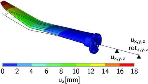
Figure 10. Elastic deformation of LC4 for statically applied loads; FZ = 1, 322 N.
Table 5 Aerodynamic load cases at Ma = 0.4 ; max. forces calculated on grid V4
The same loads applied to V1 lead to a very similar bending deformation with a 2.0 mm higher maximum deformation at the tip.
In the next step, the forced pitching motion is simulated by means of a harmonic analysis. Therefore, the aerodynamic forces are deleted and the y-rotation constraint is adapted. The equation of motion is split into two parts, namely, unknown displacements u a and prescribed displacements u b .
 $$\begin{equation}
\left( \begin{array}{cc}\mathbf {M}_{aa} & \mathbf {M}_{ab}\\
\mathbf {M}_{ba} & \mathbf {M}_{bb} \end{array} \right) \left( \begin{array}{c}\ddot{\mathbf {u}}_a\\
\ddot{\mathbf {u}}_b \end{array} \right) + \left( \begin{array}{cc}\mathbf {D}_{aa} & \mathbf {D}_{ab}\\
\mathbf {D}_{ba} & \mathbf {D}_{bb} \end{array} \right) \left( \begin{array}{c}\dot{\mathbf {u}}_a\\
\dot{\mathbf {u}}_b \end{array} \right) + \left( \begin{array}{cc}\mathbf {K}_{aa} & \mathbf {K}_{ab}\\
\mathbf {K}_{ba} & \mathbf {K}_{bb} \end{array} \right) \left( \begin{array}{c}\mathbf {u}_a\\
\mathbf {u}_b \end{array} \right) =\mathbf {0}.
\end{equation}$$
$$\begin{equation}
\left( \begin{array}{cc}\mathbf {M}_{aa} & \mathbf {M}_{ab}\\
\mathbf {M}_{ba} & \mathbf {M}_{bb} \end{array} \right) \left( \begin{array}{c}\ddot{\mathbf {u}}_a\\
\ddot{\mathbf {u}}_b \end{array} \right) + \left( \begin{array}{cc}\mathbf {D}_{aa} & \mathbf {D}_{ab}\\
\mathbf {D}_{ba} & \mathbf {D}_{bb} \end{array} \right) \left( \begin{array}{c}\dot{\mathbf {u}}_a\\
\dot{\mathbf {u}}_b \end{array} \right) + \left( \begin{array}{cc}\mathbf {K}_{aa} & \mathbf {K}_{ab}\\
\mathbf {K}_{ba} & \mathbf {K}_{bb} \end{array} \right) \left( \begin{array}{c}\mathbf {u}_a\\
\mathbf {u}_b \end{array} \right) =\mathbf {0}.
\end{equation}$$
A constant modal damping of ξ = 0.02 is defined. With the harmonic approach
 $$\begin{equation}
\mathbf {u}=\hat{\mathbf {u}}\times e^{j\omega t},
\end{equation}$$
$$\begin{equation}
\mathbf {u}=\hat{\mathbf {u}}\times e^{j\omega t},
\end{equation}$$
the equations can be rewritten as
 $$\begin{equation}
\left(-{\omega ^2} \mathbf {M}_{aa} +j\omega \mathbf {D}_{aa}+\mathbf {K}_{aa}\right)\hat{\mathbf {u}}_a = \left(\omega ^2 \mathbf {M}_{ab} -j\omega \mathbf {D}_{ab}- \mathbf {K}_{ab}\right)\hat{\mathbf {u}}_b
\end{equation}$$
$$\begin{equation}
\left(-{\omega ^2} \mathbf {M}_{aa} +j\omega \mathbf {D}_{aa}+\mathbf {K}_{aa}\right)\hat{\mathbf {u}}_a = \left(\omega ^2 \mathbf {M}_{ab} -j\omega \mathbf {D}_{ab}- \mathbf {K}_{ab}\right)\hat{\mathbf {u}}_b
\end{equation}$$
and
 $$\begin{equation}
\left(-\omega ^2 \mathbf {M}_{ba} +j\omega \mathbf {D}_{ba}+\mathbf {K}_{ba}\right)\hat{\mathbf {u}}_a = \left(\omega ^2 \mathbf {M}_{bb} -j\omega \mathbf {D}_{bb}- \mathbf {K}_{bb}\right)\hat{\mathbf {u}}_b
\end{equation}$$
$$\begin{equation}
\left(-\omega ^2 \mathbf {M}_{ba} +j\omega \mathbf {D}_{ba}+\mathbf {K}_{ba}\right)\hat{\mathbf {u}}_a = \left(\omega ^2 \mathbf {M}_{bb} -j\omega \mathbf {D}_{bb}- \mathbf {K}_{bb}\right)\hat{\mathbf {u}}_b
\end{equation}$$
As one can see from the equations above, the resulting
 $\hat{\mathbf {u}}_a$
is generally complex
$\hat{\mathbf {u}}_a$
is generally complex
 $$\begin{equation}
\mathbf {\hat{u}}_a=\mathbf {\hat{u}}_{a,Re}+j\times \mathbf {\hat{u}}_{a,Im}
\end{equation}$$
$$\begin{equation}
\mathbf {\hat{u}}_a=\mathbf {\hat{u}}_{a,Re}+j\times \mathbf {\hat{u}}_{a,Im}
\end{equation}$$
Inserting Equation (7) into Equation (4) and extracting the physically relevant real part leads to
 $$\begin{equation}
\mathbf {u}_a(t)=\Re (\mathbf {\hat{u}}_ae^{j\omega t})=\mathbf {\hat{u}}_{a,Re}\times \cos (\omega t)-\times \mathbf {\hat{u}}_{a,Im}\times \sin (\omega t)
\end{equation}$$
$$\begin{equation}
\mathbf {u}_a(t)=\Re (\mathbf {\hat{u}}_ae^{j\omega t})=\mathbf {\hat{u}}_{a,Re}\times \cos (\omega t)-\times \mathbf {\hat{u}}_{a,Im}\times \sin (\omega t)
\end{equation}$$
The deformation in z-direction of the real part
 $\mathbf {\hat{u}}_{a,Re}$
and the deformation of the imaginary part
$\mathbf {\hat{u}}_{a,Re}$
and the deformation of the imaginary part
 $\mathbf {\hat{u}}_{a,Im}$
of Equation (8) are shown in Fig. 11.
$\mathbf {\hat{u}}_{a,Im}$
of Equation (8) are shown in Fig. 11.
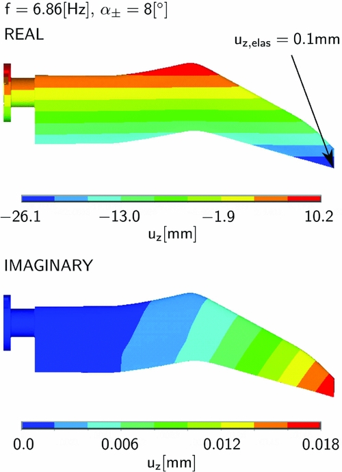
Figure 11. Harmonic motion and elastic deformation due to inertia forces.
Thanks to lightweight construction and the short chord length of the model, the moments of inertia are small, which leads to very small deformations due to harmonic motion. Because the deformation of V1 does not show any significant differences, only the deformation of V2 is presented.
The real part shows the blade tip at time t = 0, where the rotational acceleration is at its maximum. The elastic deformation is obtained by subtracting the rigid motion from the overall deformation. The maximum elastic deformation uz = 0.1 mm is small compared to the deformation due to the statically applied loads.
The imaginary part shows the blade tip at time t = T/4. The elastic deformation in the z-direction uz = 0.018 mm shows that the phase difference should be generally taken into account for high frequencies and amplitudes. For the presented case, the real part is superimposed on the static solution only, which is a conservative approach for small phase differences.
The stresses in laminate, bonding and shaft are presented for the superposed load case in the following. Both modelling approaches V1 and V2 are compared. The highest von-Mises stresses occur at the root section (Fig. 12) of the steel shaft.
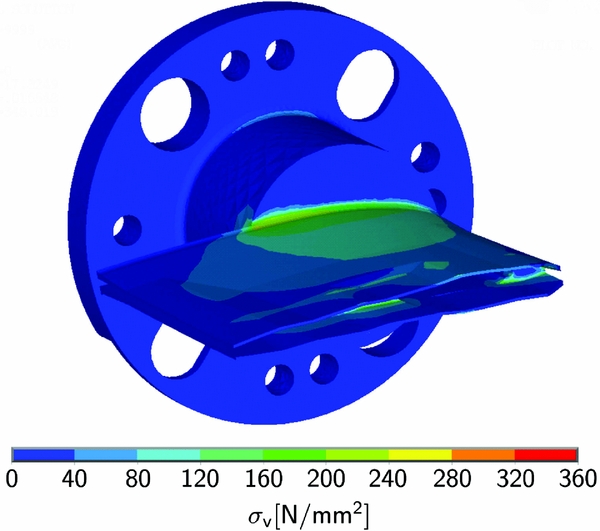
Figure 12. Von Mises stress in the steel shaft of V2.
They are nearly independent on the modelling approach. Assuming a yield point of R p0.2 = 720MPa for the 42CrMo4 steel shaft, the factor of safety is FoS = 2.
For the strength analysis of the half shells, the Puck criterion(Reference Puck and Schürmann21) is used. It identifies Fibre failure (FF) and Inter-Fibre Failure (IFF) in the unidirectional M46J lamina listed in Table 1. The out-of-plane properties of the M46J lamina and the four Puck inclination parameters are estimated with data from similar materials, while the other material properties are determined experimentally. In Fig. 13, the FF stress exposure is shown for the 2.5° spar cap layers in the upper shell. The highest physical relevant stress peaks occur at the span-wise end of the steel shaft where the loads are transferred from the spar cap to the shaft. However, the factor of safety is FoS > 3. The stress peaks show that the minimisation of the stiffness discontinuities is essential. Without the tapered channel at the span-wise end of the steel shaft, the stress exposure would be significantly higher. The stress exposure according to the IFF criterion of Puck is shown for the 90° layer of the lower half shell on the bottom of Fig. 13. The upward bending causes tensional loads in the lower half shell. Since the IFF criterion is sensitive to tensional loads, the stress exposure is highest in the 90° layer of the lower half shell. It increases towards the root where the bending moment reaches its maximum. Small discontinuities can be seen at the free corners of the spar cap reinforced shells. The effect is enforced by the neglected chord-wise tapering in the FE model. The stresses in all layers show peaks at the root section since global forces and bending moments reach their maximum. Furthermore, the material thickening of the shaft leads to a strong change in stiffness. Span-wise tapering at the root section in order to prevent edge delamination is included in the FE model.
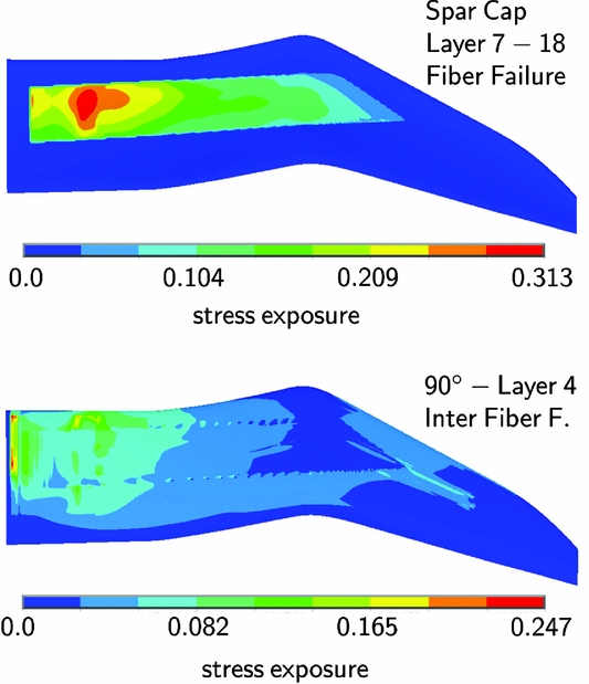
Figure 13. Strength analysis for LC4 from Section 7.
The resulting span-wise shear stress distributions τ yz of the bonding are shown in Fig. 14. Comparing the results of both modelling approaches, one can state that model V1 with the overrated bonding thickness leads to lower stress peaks than V2. The differences of the two modelling approaches are more obvious but similar to the stress distribution of the plies. In order to reduce the stress peaks in the adhesive at the span-wise end of the shaft, a channel with higher and more homogeneous tapering is introduced in V2. Furthermore, the tapering of the spar overlap is included in the V2 model and the holes in the spar are eliminated. The mean shear stress in the bonding on the upper side of the shaft is often calculated by
 $$\begin{equation}
\tau _{yz,mean}=\frac{F}{A}=\frac{18{,}873\,\mathsf {N}}{15{,}000\,\mathsf {mm^2}}=1.26 \,\mathsf {MPa},
\end{equation}$$
$$\begin{equation}
\tau _{yz,mean}=\frac{F}{A}=\frac{18{,}873\,\mathsf {N}}{15{,}000\,\mathsf {mm^2}}=1.26 \,\mathsf {MPa},
\end{equation}$$
where F are the internal section forces in span-wise direction summed over the nodes of the upper shells and A is the upper surface area of the steel shaft. The maximum mean shear stress τ yz, mean, max = 7 MPa divided by the mean shear stress of the shaft yields a factor of safety of FoS = 5.6. However, due to the inhomogeneous stress distributions shown in Fig. 14, a FoS = 2.0 seems more realistic. In the experiment, the structural FoS might be lower due to underestimated loads.
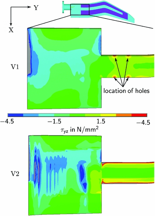
Figure 14. Shear stress τ yz in bonding on upper shaft and spar.
7.0 CFD COMPUTATIONS
Three types of computational fluid dynamic (CFD) computations with an increasing degree of complexity are presented: steady (s), unsteady (u), and unsteady cases with grid deformation (u-gd) (see Table 5). The simulations are used as load cases for the strength analysis and in order to study the occurring flow phenomena.
The CFD computations are performed by the edge-based finite-volume solver DLR-TAU(Reference Gerhold, Friedrich, Evans and Galle22). The inviscid fluxes are discretised using a second-order central scheme. A fully turbulent flow is considered. For turbulence closure, the SST k-ω turbulence model(Reference Menter23) is applied. The unstructured CFD grids are generated with CENTAUR. The same geometric properties and boundary conditions are used for all grids. Version 4 (V4) of the grid is depicted in Fig. 15.

Figure 15. CFD-grid Version 4; Geometric properties.
The grid depth equals the wind-tunnel depth of 1m. Viscous sidewalls and a farfield with radius r = 10 m (60 times the chord length) are implemented. For these conditions, the growth of the side wall boundary layers corresponds with the inflow conditions of the TWG(Reference Gardner, Richter and Rosemann25). Preliminary simulations with symmetry boundary conditions on the sidewalls are not presented because no conclusions can be drawn with respect to the separation behaviour at the wind-tunnel wall. The root aerofoils section is directly connected to the viscous wall and the gap of 1.5 mm is not taken into account.
In the first step, steady RANS simulations are carried out. A mesh convergence study is performed for case LC1 (see Table 5). The global aerodynamic coefficients and the grid properties are shown in Table 6. Above grid V2, only minor changes in the aerodynamic coefficients are given. Since the flow for this load case is attached, one might argue that a grid convergence study for unsteady cases with high angles of attack is appropriate. This investigation is beyond the scope of the work. Grid V4, presented in Fig. 15, is used for all final steady and unsteady simulations. For unsteady cases, this grid has the best convergence behaviour. The surface resolution is higher than for grid V2 and surface nodes are more physically distributed than they are in grid V1. Grid V3 was neglected because of its huge size. The value of y+ max > 1 occurs only in very small regions of the domain. Furthermore, the Reynolds number was decreased to Re = 1.2 × 10⁶ in the structural design process, which consequently leads to lower values of y+.
Table 6 LC1 computed with different grids
The basic flow features and the cp -distribution at high angles of attack can be deduced from the steady load case LC2, shown in Fig. 16. Three regions of separation can be seen on the upper blade tip surface. Hereby, it is deduced that the modification of the twist at the root is sufficient to separate wind-tunnel wall separation and first inboard separation on the model.
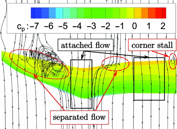
Figure 16. LC2 with grid V4; Ma = 0.4, Re = 1.2 × 10⁶, α = 15°.
In the second step, unsteady RANS computations with a rotating grid are performed. This configuration leads to fast converging results, starting with a converged steady solution. A single period is simulated with 2,000 physical time steps per period and 100-1,000 inner iterations, depending on a Cauchy convergence criterion. In order to check the influence of the different grids, LC3 is simulated with grids V1, V3 and V4 (Fig. 17). More than two periods are only calculated with grid V1 in order to check periodicity. The second period is already in good agreement with the third period, as shown in Fig. 17. Grids V3 and V4 show a better agreement in the lift coefficient peaks C L, peak , which are significantly higher than in the steady case. However, the re-attachment region differs significantly, and a second lift peak is only resolved by grid V3, which is probably less dissipative. Due to the lower number points and its numerical robustness, grid V4 is used for all further simulations. The unsteady load case presented above yields a maximum global force F Z, max = 1, 766 N. This leads to a violation of the safety margin in the FE analysis (see above). Therefore, the Reynolds number is reduced by 25% for load case LC4 (see Table 5), which was used for the final strength analysis.
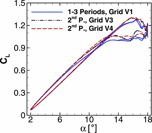
Figure 17. LC3: Ma = 0.4, Re = 1.6 × 10⁶; CL − α distribution for different grids.
Comparing the CL − α distribution at Re = 1.6 × 10⁶ in Fig. 17 to the CL − α distribution at Re = 1.2 × 10⁶ in Fig. 18, no significant differences can be seen. In order to save computational costs, one could have equally reduced the forces of LC3 by 25% for the final strength analysis. The delayed and increased lift peak in comparison to the steady case is clearly visible. There is no significant global pitching moment peak in the CMy − α distribution as presented for the 2D cases in Gardner et al(Reference Gardner, Richter, Mai, Altmikus, Klein and Rohardt2).
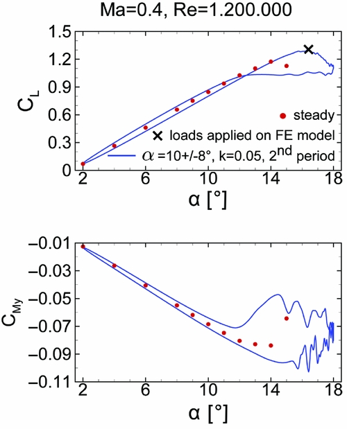
Figure 18. LC4: Ma = 0.4, Re = 1.2 × 10⁶; CL − α distribution (top), CMy − α distribution (bottom).
The rotating viscous sidewalls do not match the non-rotating wind-tunnel walls because they introduce momentum into the domain (no-slip condition). Therefore, unsteady RANS computations with grid deformation are carried out using the DLR-TAU deformation tool, which is based on radial basis functions(Reference Gerhold and Neumann24). All surface points of the aerodynamic mesh of the blade tip are moved in a rigid body motion. The instantaneous flow fields at α inst = 16.08°↗ computed with rotating sidewalls and with grid deformation technique are compared in Fig. 19. The differences in the pressure distribution cp and in the streamlines are so small that the simulation configuration with the rotating grid seems accurate enough to investigate the flow phenomena of the pitching blade tip. Comparing the FZ -peak of one period, the difference is ΔF Z, peak = 12 N, which is negligible for structural design criteria.
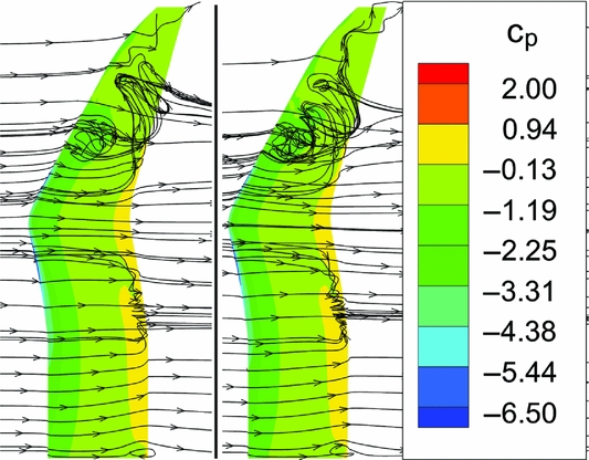
Figure 19. LC4 at α inst = 16.08°↗; Grid deformation (left) vs rotating grid (right).
The flow phenomena, shown in Fig. 19, are similar to the flow phenomena of the steady case, shown in Fig. 16. The tip vortex merges with the dynamic stall vortex of the backward swept part. A smaller inboard separation occurs at r ≈ 250 mm at the trailing edge. Inner and outer vortices pass the trailing edge at different angles of attack. Therefore, no single pitching moment peak appears in Fig. 18. There are two regions of attached flow: one at the notch and one between the corner stall at the root and the desired separation region at r ≈ 250 mm.
8.0 EXPERIMENTAL VALIDATION OF CFD COMPUTATIONS
Figure 17 depicts the grid dependency of the computational results as soon as soon as separation sets in. Using other turbulence models does not necessarily improve the results. The uncertainty and the lack of accuracy concerning the separation behaviour in CFD computations are one main reason for the continuing demand for wind-tunnel experiments. In this section, the numerical set-up is validated by experimental results. The global forces and moments measured by the piezo balance and the unsteady pressure transducers in the span-wise cross-sections 2, 4 and 6 (see Fig. 2) are evaluated. Due to limitations in the hydraulic oscillation rig, it was not possible to reach an oscillation amplitude of 8° at k = 0.05 in the experiment. Therefore, load cases LC6 and LC7 are used for the comparison of the numerical and experimental results. Table 7 lists the considered load cases.
Table 7 Aerodynamic load cases at Ma = 0.5 ; max. forces calculated on grid V4
In Fig. 20, the steady polar at Ma = 0.5 and Re = 1.2 × 10⁶ is shown. The measured global lift and moment coefficients are in a good agreement with the numerical data. However, separation sets in earlier in the numerical computations, which can be deduced from the nonlinear behaviour in the lift starting at α ≈ 12.0°. The experimental lift increases almost linearly up to the last measured point at α ≈ 12.5°. At this point, the augmentation of the standard deviation of the lift and moment coefficient indicates separation. Due to the high peak loads, no measurements are possible at higher angles of attack. The pitching moment coefficient is nearly zero at α ≈ 0.0° and reaches its nose-down minimum C My, min ≈ −0.075 at α ≈ 12.0°. The moment coefficient C My, exp is slightly lower in the computation as long as the flow stays attached.
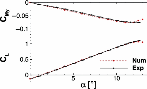
Figure 20. Global lift and pitching moment polar of LC6.
In Fig. 21, the global lift and moment coefficient for a light dynamic stall case at Ma = 0.5, Re = 1.2 × 10⁶ and α = 8° ± 5° are shown. On the experimental side, the phase average and standard deviation of CL and CM over 160 periods are presented. The experimental pitching frequency is fexp = 6.6 Hz, which leads to a period length of T = 0.1515 s. The experimental and numerical curves start at the same angle-of-attack. The corresponding experimental angle-of-attack is plotted for convenience. The numeric pitching frequency is fnum = 6.5 Hz, which yields a difference of Δf exp, num = 1.5%. In the regions of attached flow, the numerical and experimental data show a good agreement for CL . However, as soon as separation sets in, the lift is underestimated by the computations. The numerical lift peak is 5.4% higher than in the numerical static polar. As in the steady case, the simulations show an earlier drop of the lift at t = 0.03 s. After t = 0.03 s, oscillations occur in the experimental and numerical data. In case of C L, exp , this can be seen at the downstroke where the standard deviation of CL is significantly increased. The maximum lift peak has a strong variation over all periods. Its absolute maximum is C L, max = 1.49. It is 33% higher than the numerical lift peak, which reduces the overall factor of safety from FoS = 2.0 to FoS = 1.5. The aerodynamic oscillations caused by vortices travelling across the blade excite eigenfrequencies of the wind-tunnel model. In the pitching moment, the higher harmonic oscillations near the second eigenfrequency are evident. This behaviour cannot be captured by the CFD simulation with the rigid contour. However, similar tendencies can be seen for CM : a stronger nose-down moment for the first half of the period, a less strong moment for the second half of the period.
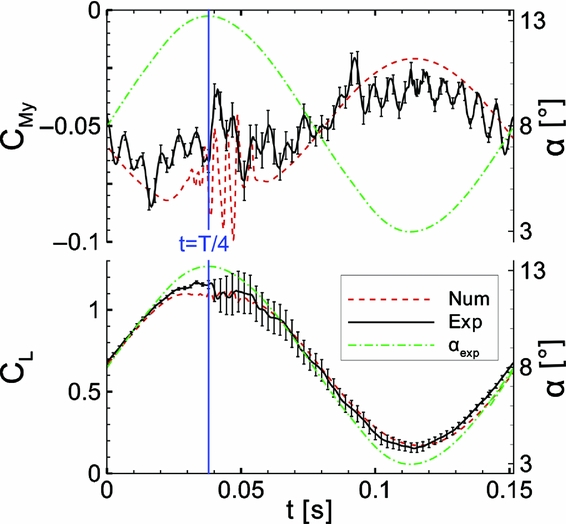
Figure 21. Unsteady lift and pitching moment for LC7.
In Fig. 22, two instantaneous cp -distributions are shown for three span-wise sections. The angle-of-attack is α = 8° at t = 0 and α = 13° at t = T/4. As mentioned in Section 1, the angle-of-attack refers to the angle of the chord at zero twist (r = 0.39 m) to the direction of the inflow. Compared to the notch section and the inboard section, the outboard section S6 at r = 0.525 m shows the highest numerical and experimental suction peak for both points of time. At t = T/4, the increased standard deviation at sensor three and four indicate a shock-induced laminar separation bubble. The computations do not resolve the laminar separation bubble but show large separation from x/c = 0.3 to the trailing edge at t = T/4. The experimental and numerical results at sections S2 and S4 show an excellent agreement, although the computations are fully turbulent and with a rigid geometry. The critical pressure coefficient for Ma = 0.5 is c p, krit = 2.13. A light shock between x/c = 0.1 and x/c = 0.15 at S4 for t = T/4 is not resolved by the RANS calculations.

Figure 22. cp -distributions at span-wise sections for LC6; α unst (t = 0) = 8° and α unst (t = T/4) = 13°.
9.0 CONCLUSIONS
The aerodynamic and structural design of a pitching double-swept rotor blade tip for the investigation of 3D dynamic stall in the transonic wind tunnel (TWG) is presented. The carbon fibre reinforced plastic model and its FE analysis concerning deformation, stress and eigenmodes are shown. The FE model is validated by an experimental modal analysis. Fully turbulent RANS simulations are presented for Ma = 0.4 and Ma = 0.5. A light dynamic stall at Ma = 0.5 is compared to experimental data.
-
• A span width of b = 750 mm and an aspect ratio of 4.7 lead to a very limited instrumentation space and highly loaded carbon composite shells.
-
• Two FE modelling approaches of different complexity are proposed for the adhesive between the outer half shells and the inner components. The fast and easy approach is well suited for the pre-design because the weakest spots can be detected and a first estimation of eigenfrequencies and mode shapes is possible. However, the more sophisticated approach should be used for the final strength analysis because this approach is conservative and stresses are not underestimated.
-
• The experimental modal analysis shows an excellent agreement to the results of the FE model. The first mode shape (bending) is at f = 70 Hz, the first pure torsional mode at f = 434 Hz. Thus, the model is considered to be relatively stiff, the aeroelastic influence is low.
-
• For statically applied unsteady aerodynamic loads (Ma = 0.4, Re = 1.2 × 10⁶, α inst = 16.08°) the deformation is almost pure bending and reaches 18 mm at the tip.
-
• An overall strength analysis including Puck criterions is shown. The shear stresses τ yz in the adhesive limit the possible load cases. A simple averaged calculation of the mean shear stress is not conservative for inhomogeneous stress distributions. The simulated light dynamic stall case at Ma = 0.5 and Re = 1.2 × 10⁶ yields a factor of safety of FoS = 2.0 for the FE model.
-
• Fully turbulent, unsteady RANS computations with the rigid geometry show three regions of separated flow: one outboard of the notch, one inboard of the notch and one at the wind-tunnel wall. The inboard dynamic stall is not triggered by the wind-tunnel wall separation because of the reduced twist at the root.
-
• The unstady RANS simulations show a grid dependency at high angles of attack and separated flow. However, the lift peaks are nearly at the same magnitude, so the simulations are well suited for design purposes.
-
• The global lift and moment polar for Ma = 0.5 and Re = 1.2 × 10⁶ show an excellent agreement between numerical and experimental results. The simulations indicate separation at slightly lower angles of attack than the experiment.
-
• Due to the earlier separation in the computations, the experimental global peak forces are 33% higher for Ma = 0.5 α = 8 ± 5° and f = 6.6 Hz. Thus, the factor of safety is reduced from FoS = 2.0 to FoS = 1.5. This is the limit taking into account further uncertainties in the composite materials. Therefore, one can state that a factor of safety of FoS = 2.0 is necessary but sufficient for the design of this experiment and the presented computational methods. If there is a stronger uncertainty for the aerodynamic loads, an online monitoring of the global forces is recommended during the experiment.
ACKNOWLEDGEMENTS
This work is funded by the DLR programmatic research in the project ‘STELAR’. The authors would like to acknowledge the support and help of H. Mai, T. Büte, A. Benkel and J. Sinske during the experiment. The authors would like to thank A. D. Gardner, Y. Meddaikar, F. Wienke and M. Fehrs for the paper correction.


