


Results from the 2020 Census led to a new round of House apportionment: New York, California, Illinois, West Virginia, Michigan, Ohio, and Pennsylvania lost one seat; Montana, Florida, Colorado, North Carolina, and Oregon gained one seat; and Texas gained two seats. Careful readers of the apportionment results noticed that New York, with a population of more than 20 million, lost its one seat by an extremely small margin. That is, if the Census had counted 89 more people in the state’s population, New York would not have lost any of its original 27 seatsFootnote 1; instead, Minnesota would have lost one seat. Some scholars argue that New York’s loss was a direct result of an unfairly conducted Census because the Trump administration attempted to add a citizenship question to the questionnaire and shortened the counting period by a month. Both decisions likely contributed to an undercounting of minorities and immigrants, groups that are overrepresented in states such as New York. Even without these changes, it was likely that the 2020 Census undercounted minorities and immigrants regardless for reasons ranging from the inherent bias of the enumeration method, “actual inquiry at every dwelling-house” as opposed to statistical sampling,Footnote 2 to the negative impact of the COVID-19 pandemic.
These counting-related issues attracted significant attention because they directly impacted the Census results and the downstream applications, such as the apportionment of the US House of Representatives. The apportionment method drew less attention in part because it has been unchanged since 1941, when an amendment to the Permanent Apportionment Act of 1929 established the officially named “Equal Proportions Method”—also known as Huntington-Hill’s method—as the current apportionment method. For many, the apportionment method appears to be a simple technical matter: once the 2020 Census results were determined, the numbers were input into the Equal Proportions Method and the new “equally proportioned” apportionment numbers were the result.
Overlooking the apportionment method would be a significant omission, however, because—contrary to common belief—the US House of Representatives in fact is malapportioned, and different methods result in different levels of malapportionment. It is easily understood that the apportionment of the House—that is, the distribution of 435 House seats among 50 states—cannot be perfectly proportional to the population because the number of seats for each state must be a positive whole number. Consequently, the proportion of a state’s House seats relative to the total number cannot always match the proportion of a state’s population relative to the national population. For example, South Carolina has seven House seats and a population of 5,124,712, according to the 2020 Census.Footnote
3 The state’s share of House seats is
 $ \frac{7}{435}\hskip0.35em =\hskip0.35em 1.609\% $
, whereas its share of the population is
$ \frac{7}{435}\hskip0.35em =\hskip0.35em 1.609\% $
, whereas its share of the population is
 $ \frac{\mathrm{5,124,712}\;}{\mathrm{331,108,434}}\hskip0.35em =\hskip0.35em 1.547\% $
; thus, South Carolina is slightly overrepresented in the House. Ideally, this inevitable malapportionment would be random among states regardless of population size so that neither more populous nor less populous states are systematically disadvantaged because of the apportionment method used. However, the malapportionment among states is not random. The current apportionment method is biased against more populous states, and states such as New York lost one seat in 2020 as a result.
$ \frac{\mathrm{5,124,712}\;}{\mathrm{331,108,434}}\hskip0.35em =\hskip0.35em 1.547\% $
; thus, South Carolina is slightly overrepresented in the House. Ideally, this inevitable malapportionment would be random among states regardless of population size so that neither more populous nor less populous states are systematically disadvantaged because of the apportionment method used. However, the malapportionment among states is not random. The current apportionment method is biased against more populous states, and states such as New York lost one seat in 2020 as a result.
The current apportionment method is biased against more populous states, and states such as New York lost one seat in 2020 as a result.
Historically, the United States has used four different apportionment methods that fall into two categories: Hamilton’s method (a quota method), Huntington-Hill’s method (a divisor method), Jefferson’s method (a divisor method), and Webster’s method (also a divisor method).Footnote
4 All quota methods start with the standard quota of each state. For example, because South Carolina has
 $ 1.547\% $
of the total population based on the 2020 Census, its standard quota is
$ 1.547\% $
of the total population based on the 2020 Census, its standard quota is
 $ 1.547\% $
of House seats, which is
$ 1.547\% $
of House seats, which is
 $ 1.547\% $
×435=6.729 seats. Because it is not possible to apportion 6.729 seats to a state, Hamilton’s method works by first giving every state its lower quota (e.g., in the case of South Carolina, its lower quota is six) and then distributing the remaining seats one at a time to states based on the size of their leftover quota fractions (e.g., South Carolina’s leftover fraction is 0.729). A divisor method works by dividing the state populations by a modified divisor to obtain modified quotas and then rounding the modified quotas to whole numbers using a predetermined rounding method. For example, a modified divisor that works for Huntington-Hill’s method for the 2020 apportionment is 762,995. Thus, South Carolina has a modified quota of
$ 1.547\% $
×435=6.729 seats. Because it is not possible to apportion 6.729 seats to a state, Hamilton’s method works by first giving every state its lower quota (e.g., in the case of South Carolina, its lower quota is six) and then distributing the remaining seats one at a time to states based on the size of their leftover quota fractions (e.g., South Carolina’s leftover fraction is 0.729). A divisor method works by dividing the state populations by a modified divisor to obtain modified quotas and then rounding the modified quotas to whole numbers using a predetermined rounding method. For example, a modified divisor that works for Huntington-Hill’s method for the 2020 apportionment is 762,995. Thus, South Carolina has a modified quota of
 $ \frac{\mathrm{5,124,712}\;}{\mathrm{762,995}}\hskip0.35em =\hskip0.35em $
6.716. Because Huntington-Hill’s method uses geometric rounding, 6.716 is rounded up to 7 because this modified quota is greater than its geometric mean, which is
$ \frac{\mathrm{5,124,712}\;}{\mathrm{762,995}}\hskip0.35em =\hskip0.35em $
6.716. Because Huntington-Hill’s method uses geometric rounding, 6.716 is rounded up to 7 because this modified quota is greater than its geometric mean, which is
 $ \sqrt{6\times 7}\hskip0.35em =\hskip0.35em 6.480 $
.
$ \sqrt{6\times 7}\hskip0.35em =\hskip0.35em 6.480 $
.
Applying different apportionment methods to the 2020 Census leads to dramatically different outcomes, as shown in figure 1. Webster’s method, the only unbiased divisor method (Balinski and Young Reference Balinski and Young2001), would have led to changes in four states compared to the current method. New York and Ohio would have gained one seat each, preserving their respective 27 and 16 seats from the 2010 Census, whereas Montana and Rhode Island would have lost one seat each. Jefferson’s method, with a bias in favor of more populous states, would have led to changes in 14 states. Among the changes, California, Texas, and New York would have gained two seats and eight states would have lost one seat.Footnote 5
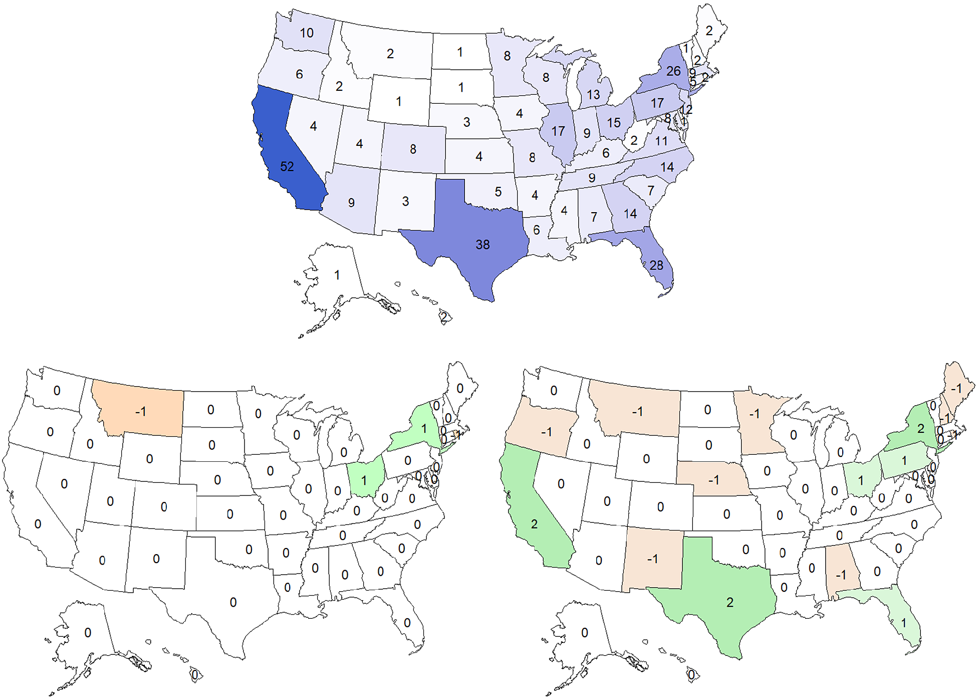
Figure 1 Different Apportionment Outcomes under Different Methods, 2020
(1) Top: Apportionment results are based on the current (i.e., Huntington-Hill’s) apportionment method. Darker colors indicate more seats. (2) Bottom left: Changes are from the current method to Webster’s method. Orange indicates seat loss; green indicates seat gain. (3) Bottom right: Changes are from the current method to Jefferson’s method. Orange indicates seat loss; green indicates seat gain.
The choice of an apportionment method is ideally a priori and based on a method’s mathematical properties instead of its short-term political implications. If the apportionment method is not to be changed every few years based on what benefits the party in power at the time, it is necessary to have criteria to evaluate potential methods. Balinski and Young (Reference Balinski and Young2001) developed the criteria of within-quota, consistency, and unbiasedness, among others. In simple terms, “within-quota” means that the actual number of seats that a state receives (i.e., a positive whole number) should be close to the theoretical number of seats that a state is supposed to receive (i.e., its standard quota, unlikely to be a positive whole number); therefore, the actual number of seats should be either the lower or the upper quota. South Carolina has a standard quota of 6.729 seats based on the 2020 Census; therefore, it has a lower quota of six and an upper quota of seven, the two nearest integers to the standard quota. The within-quota criterion requires South Carolina to have six or seven seats. Assigning fewer than six seats or more than seven seats would violate the within-quota criterion.
The consistency criterion requires an apportionment method to behave predictably when the size of the US House of Representatives and/or the size of the population changes. The requirements relating to House size and population size are known as “house monotonicity” and “population monotonicity,” respectively. If the House increases in size, it would require a new apportionment. The house monotonicity criterion requires that because there are more seats to be distributed among the same states, no state should lose a seat(s) as a result of the new apportionment. In other words, if the House increases in size—for example, from 435 to 500—and the population remains the same, then South Carolina, which currently has seven seats, should be able to keep at least all of its seven seats without losing any and with the possibility of gaining a few. If South Carolina loses one or even a few seats when the House increases in size, then the responsible apportionment method would be violating house monotonicity and, therefore, the consistency criterion. Population monotonicity means that if one state gains a seat(s) and another state loses a seat(s), it must be the result of the first state gaining population relative to the second state. The violation of population monotonicity also means the violation of the consistency criterion.
The unbiasedness criterion is closely connected to the US Supreme Court’s “one person, one vote” principle in that it requires no state—regardless of population size—to be systematically advantaged or disadvantaged as a result of apportionment. In every apportionment, some states received more than their standard quota, such as South Carolina in 2020, and others received less. Theoretically, the gains and the losses should be random in terms of state population size. In other words, if an apportionment method consistently leads to larger districts (e.g., an average of 800,000 constituents per district) in more populous states and smaller districts (e.g., an average of 700,000 constituents per district) in less populous states, it would be considered biased against more populous states because an individual in a more populous state would have less voice compared to an individual in a less populous state.Footnote 6
Although all three criteria may seem desirable for selecting an apportionment method, Balinski and Young (Reference Balinski and Young2001) demonstrated that, unfortunately, it is not possible for an apportionment method to satisfy both the within-quota and the consistency criteria. Because of this inevitable tradeoff, the United States had oscillated between Hamilton’s method, which stays within quota but is not consistent, and a divisor method (e.g., Jefferson’s or Webster’s), which is consistent but violates the within-quota rule. After long arguments mired with deep confusion, Congress decided in the 1910s that inconsistency was a greater evil compared to out-of-quota and rejected Hamilton’s method as a result.
After rejecting Hamilton’s method, Congress took more than two decades to eventually codify Huntington-Hill’s method as the official apportionment method in 1941. Congress believed at the time that Huntington-Hill’s method was both a consistent method and the least biased method in its category of divisor methods; however, the latter belief is untrue.Footnote 7 All divisor methods, including Huntington-Hill’s method, are consistent. The least biased divisor method, however, is not Huntington-Hill’s but rather Webster’s method. Huntington-Hill’s method is biased in favor of less populous states, and the fact that New York lost a seat to Minnesota as a result of the 2020 Census perfectly illustrates this bias. Scholars including social scientist Walter Wilcox disputed the erroneous notion that Huntington-Hill’s method was the least biased divisor method as early as 1928, and mathematicians, economists, legal scholars, and political scientists have since demonstrated repeatedly the validity of his original argument. However, Huntington-Hill’s method was adopted and continues to serve as the official apportionment method. It has produced nine apportionment results since its adoption, eight of which are biased in favor of less populous states. Webster’s method should replace Huntington-Hill’s method as the official apportionment method because, as Wilcox stated, “If the main purpose is, as it probably was in the Constitutional Convention of 1787, to hold the balance even between the large and the small states as groups, that end is best secured by the method of Webster” (Balinski and Young Reference Balinski and Young2001, 55).
Webster’s method should replace Huntington-Hill’s method as the official US apportionment method because, as Wilcox stated, “If the main purpose is, as it probably was in the Constitutional Convention of 1787, to hold the balance even between the large and the small states as groups, that end is best secured by the method of Webster.”
HAMILTON’S METHOD AND THE TRADEOFF BETWEEN WITHIN QUOTA AND CONSISTENCY
The essential task of an apportionment method is to distribute all of the US House of Representatives seats among the states in a way that resembles proportional representation. Consider the example illustrated in table 1. Three states—Large, Medium, and Small—share a total population of 1 million and a total of 100 House seats. To begin, an intuitive rule of thumb is the within-quota rule. Because Large State has 55.22% of the population, it makes sense that it also should have approximately 55.22% of the House seats, which is either 55 (lower quota) or 56 seats (upper quota). If Large State’s seat number is fewer than 55 or more than 56, then this violates the within-quota rule and deviates from an intuitive approximation of proportional representation.
Table 1 Hamilton’s Method

Note: Standard divisor/average district size: 10,000.
Hamilton’s method is structured such that it always satisfies the within-quota rule. His method first divides the states’ populations by the standard divisor (i.e., the average district size) to give each state a standard quota. It then rounds the standard quota down to the nearest integer (i.e., if the standard quota is less than 1, it rounds up to 1) and distributes any remaining seats one at a time to states with the highest leftover fractions. Hamilton’s method always satisfies the within-quota rule because it first gives states their lower quota, thereby guaranteeing not going below the lower quota, and it allows the addition of at most one seat on top of the lower quota, thereby never exceeding the upper quota.
Despite satisfying the within-quota rule and therefore intuitively approximating proportional representation, Hamilton’s method violates both aspects of the consistency criterion: house monotonicity and population monotonicity. The house monotonicity criterion stipulates that if the population remains the same and the House size increases thereby requiring a new apportionment, then no states should lose a seat(s) as a result between the original and the new apportionment. This criterion makes intuitive sense: because the same states now have more House seats to share among them, some states should be better off by gaining a seat(s), other states should remain the same, and no states should be worse off by losing a seat(s). However, this is not what would have happened in Alabama in 1880 using Hamilton’s method. It was discovered that if the House size were to increase from 299 to 300 in 1880 and the population remained the same, the State of Alabama would have lost one seat, decreasing from eight to seven using Hamilton’s method.Footnote 8
The population monotonicity criterion stipulates that if one state gains a seat(s) and another state loses a seat(s) in a new round of apportionment, then this must be the result of the first state gaining population relative to the second state.Footnote 9 If one state gains a seat(s) and another state loses a seat(s) but the state populations remain the same—or worse, the first state lost population relative to the second state—this would violate the population monotonicity criterion. The Oklahoma Paradox serves as an example of such a violation. When the State of Oklahoma joined the Union as the 46th state in 1907, its population was estimated at approximately 1 million and the standard divisor (i.e., the average House district size) was approximately 193,000. It therefore was decided that the House size should increase by five seats, from 386 to 391, to accommodate the new state. Using Hamilton’s method, Oklahoma indeed would acquire exactly five seats in 1910; however, New York also would lose a seat to Maine, even though New York’s and Maine’s populations remained the same. The Oklahoma Paradox, also known as the New State Paradox, is an example of the violation of the population monotonicity criterion because when one state (Maine) gained a seat and another (New York) lost a seat, it was not because Maine gained population relative to New York, which was required by the population monotonicity criterion. Maine’s population remained the same as did New York’s.Footnote 10
The New State Paradox was the breaking point that led Congress to discontinue the use of Hamilton’s method in the 1910s. Despite its intuitive appeal (i.e., it satisfies the within-quota rule), Hamilton’s method is inconsistent (i.e., it violates both the house monotonicity and population monotonicity criteria), which could cause problems and raise objections. Is there a method that is both within quota and consistent? Unfortunately, the answer is no because the Balinski and Young impossibility theorem demonstrated that it is not possible for an apportionment method to satisfy both the within-quota and population-monotonicity criteria.Footnote 11 A choice was made: when Congress discontinued the use of Hamilton’s method in the 1910s, it decided to permanently move to divisor methods, which are consistent but may violate the within-quota criterion.Footnote 12
DIVISOR METHODS AND BIAS IN TERMS OF STATE POPULATION
The United States completed its first congressional apportionment using Jefferson’s method. Jefferson’s method first divides state populations by a modified divisor to obtain a modified quota for each state and then rounds the quotas down to whole numbers to obtain the number of seats for each state. Because the number of seats for all of the states must add up to exactly the size of the House, the key is to find a modified divisor that satisfies this requirement. In the example shown in table 2, a modified divisor of 9,850 satisfactorily apportions a total of 100 House seats using Jefferson’s method.
Table 2 Divisor Methods

Other divisor methods including Webster’s and Huntington-Hill’s work in a similar manner, with the only difference being the method of rounding. A modified divisor first divides state populations into modified quotas, which then are rounded to whole numbers to obtain the number of seats for each state such that the total number adds up to the size of the House.Footnote
13 For Webster’s method, the rule for rounding is arithmetic rounding: that is, a number with a fraction equal or greater to 0.5 is rounded up and the remainder are rounded down. For Huntington-Hill’s method, the rule for rounding is geometric rounding: that is, for a number to round up, it must be greater than the square root of the product of its two nearest integers. For example, to determine whether a modified quota of 55.44 should be rounded up or down using Huntington-Hill’s method, 55.44 is compared to
 $ \sqrt{55\times 56}\hskip0.35em =\hskip0.35em 55.49 $
and, because 55.44 < 55.49, the quota is rounded down to 55.
$ \sqrt{55\times 56}\hskip0.35em =\hskip0.35em 55.49 $
and, because 55.44 < 55.49, the quota is rounded down to 55.
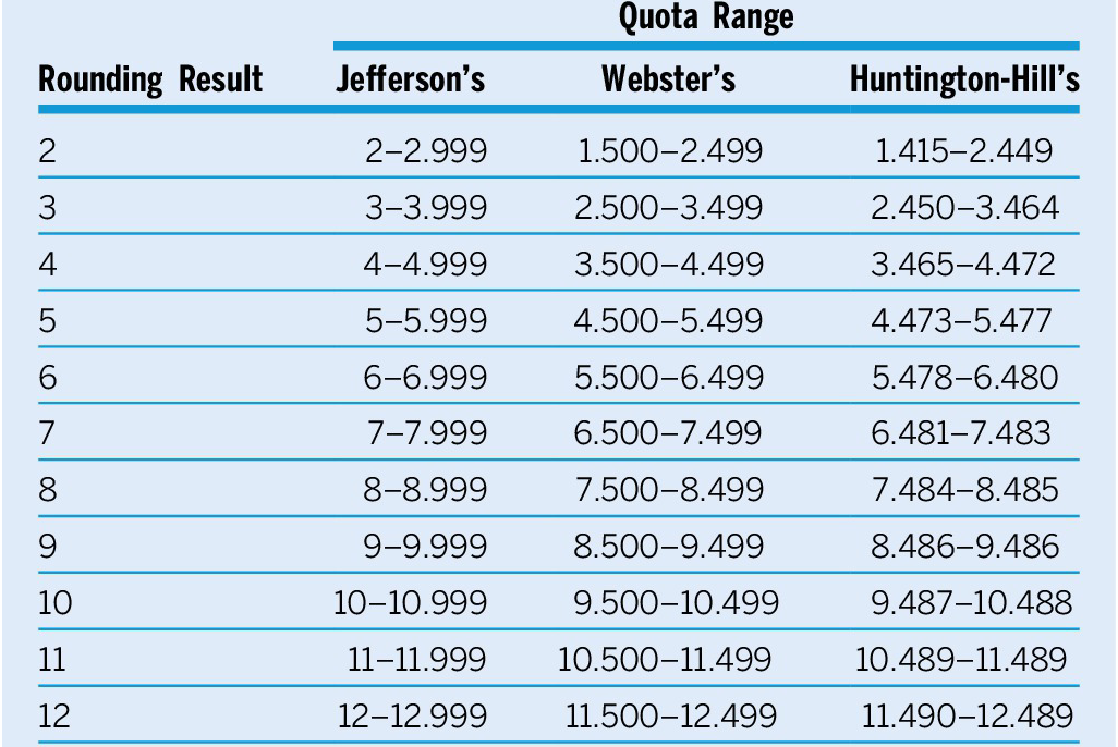
The biases of divisor methods in terms of state population size are in their rounding methods because different methods require different thresholds for rounding up or down. Table 3 shows the rounding thresholds for the three methods discussed previously. Because Jefferson’s method always rounds down, it is biased in favor of more populous states. When two states lose the same fraction as the result of rounding down, the more populous state loses less in proportion to its total quota.
Table 3 Comparing Rounding Methods
Webster’s method is unbiased (i.e., the only unbiased divisor method) in terms of state population because it allows for rounding up as well as rounding down to the nearest integer, thereby allowing the greater loss of less populous states to be offset by their greater gain.Footnote
14 Huntington-Hill’s method is biased in favor of less populous states because its fractional threshold for rounding up is not a constant; it is smaller for less populous states and larger for more populous states. Because of the different thresholds, the relative losses of less populous states are less than their relative gains. Consider this example: for a less populous state to round down to two seats, it loses at most
 $ \frac{0.45}{2.45}\hskip0.35em =\hskip0.35em 18.36\% $
of its quota; for a less populous state to round up to two seats, it gains at most
$ \frac{0.45}{2.45}\hskip0.35em =\hskip0.35em 18.36\% $
of its quota; for a less populous state to round up to two seats, it gains at most
 $ \frac{2-1.415}{1.415}\hskip0.35em =\hskip0.35em 34.27\% $
of its quota. Therefore, a less populous state’s potential gain is greater than its potential loss; the reverse is true for a more populous state.
$ \frac{2-1.415}{1.415}\hskip0.35em =\hskip0.35em 34.27\% $
of its quota. Therefore, a less populous state’s potential gain is greater than its potential loss; the reverse is true for a more populous state.
The bias of Huntington-Hill’s method against more populous states is illustrated by the latest apportionment result. Based on the 2020 Census and a modified divisor of 762,995, New York and Minnesota have modified quotas of 26.49526 and 7.48334, respectively (table 4). Although New York’s quota has a larger fraction (0.49526>0.48334), it also faces a larger threshold for rounding up because it is a more populous state. The threshold for New York is
 $ \sqrt{26\times 27}\hskip0.35em =\hskip0.35em 26.49528 $
and the threshold for Minnesota is
$ \sqrt{26\times 27}\hskip0.35em =\hskip0.35em 26.49528 $
and the threshold for Minnesota is
 $ \sqrt{7\times 8}\hskip0.35em =\hskip0.35em 7.48331 $
. Because of the bias in favor of less populous states, New York ultimately rounded down to 26 seats and Minnesota rounded up to eight seats.
$ \sqrt{7\times 8}\hskip0.35em =\hskip0.35em 7.48331 $
. Because of the bias in favor of less populous states, New York ultimately rounded down to 26 seats and Minnesota rounded up to eight seats.
Table 4 New York and Minnesota, Apportionment Results Based on the 2020 Census

Because of the bias of the current apportionment method in favor of less populous states, congressional district sizes are smaller in less populous states. As table 4 indicates, the average district size in Minnesota is significantly smaller than in New York; the difference is even greater if states such as Rhode Island and Montana are considered (i.e., the average district size for Rhode Island is 549,081 and for Montana is 542,703). From a different perspective, less populous states have greater shares of House representation: Minnesota has
 $ \frac{\mathrm{5,709,752}}{\mathrm{331,108,434}}\hskip0.35em =\hskip0.35em 1.724\% $
of the national population and
$ \frac{\mathrm{5,709,752}}{\mathrm{331,108,434}}\hskip0.35em =\hskip0.35em 1.724\% $
of the national population and
 $ \frac{8}{435}\hskip0.35em =\hskip0.35em 1.839\% $
of House seats; New York has
$ \frac{8}{435}\hskip0.35em =\hskip0.35em 1.839\% $
of House seats; New York has
 $ \frac{\mathrm{20,215,751}}{\mathrm{331,108,434}}\hskip0.35em =\hskip0.35em 6.105\% $
of the national population and
$ \frac{\mathrm{20,215,751}}{\mathrm{331,108,434}}\hskip0.35em =\hskip0.35em 6.105\% $
of the national population and
 $ \frac{26}{435}\hskip0.35em =\hskip0.35em 5.977\% $
of House seats.
$ \frac{26}{435}\hskip0.35em =\hskip0.35em 5.977\% $
of House seats.
Table 5 is an overview of the apportionment methods against the evaluation criteria, which is a two-step process for the selection of an apportionment method.Footnote 15 First, because it is not possible for a method to satisfy both the within-quota and the consistency criteria, a choice must be made between the two. Congress decided to choose consistency, which meant rejecting Hamilton’s method and accepting divisor methods. Second, because all divisor methods are consistent but have different biases, the methods must be evaluated against the unbiasedness criterion. Congress failed in this regard and chose Huntington-Hill’s method over Webster’s method in 1941, even though Webster’s method was the only unbiased divisor method.
Table 5 Apportionment Methods Against Evaluation Criteria

Notes: *Overlapping years indicate that two methods agreed and no official distinction was made. Missing years indicate no apportionment.
THE BIAS OF RECENT APPORTIONMENT RESULTS AND THE PROPOSED SOLUTION
Since its official adoption in 1941, the bias of Huntington-Hill’s method against more populous states was evident in eight of the nine apportionments, compared to the results obtained using Webster’s method. Table 6 shows that between 1940 and 2020, Huntington-Hill’s method and Webster’s method agreed only once, in 2000. Otherwise, at least one and sometimes two populous states lost a seat to less populous states. This bias has serious, long-lasting ramifications, disadvantaging more populous states in almost all aspects of federal politics ranging from congressional representation to the Electoral College.
Table 6 Apportionment Results under Different Methods, 1940–2020*

Note: *Apportionment results for 1940–2000 were obtained from Balinski and Young (Reference Balinski and Young2001). Apportionment results for 2010 and 2020 were calculated by the author.
Although the current apportionment method is demonstrably biased against more populous states, it has received surprisingly little attention considering the significance of its impact. Those who did become aware of the different apportionment methods and their respective properties were duly alarmed. “It cannot be said that reason and mathematics dictated the choice of the method that we use today in the United States.…So we find ourselves today uncomfortably uncertain if the arguments in favor of our current policy on apportionment are cogent, persuasive, or rigorous” (Robinson and Ullman Reference Robinson and Ullman2016, 222). Some scholars argued that Webster’s method should be implemented instead because it is the only unbiased divisor method (Agnew Reference Agnew2008; Balinski and Young Reference Balinski and Young2001), whereas others—more radically—argued for Jefferson’s method to create advantages in favor of more populous states to offset the disadvantages that they accrued in the Senate and in the Electoral College (Gaines and Jenkins Reference Gaines and Jenkins2009).
On balance, the argument favors Webster’s method both mathematically and pragmatically. Mathematically, Webster’s method is the only unbiased divisor method and, therefore, the best candidate to achieve proportional representation. Pragmatically, Webster’s method has the advantage of using a simple rounding method and therefore is more likely to be understood by the public as well as by members of Congress. The difference in apportionment results between Huntington-Hill’s method and Webster’s method also is relatively small, which might increase Webster’s appeal as a non-radical and viable alternative.
Ideally, the choice of an apportionment method should be a priori and based on the method’s properties instead of its short-term political implications. However, it is only an ideal—ultimately, any decision to change the apportionment method will be political. In 1941, Webster’s method lost to Huntington-Hill’s method in part because of an erroneous understanding of the apportionment methods’ mathematical properties, in part because of Harvard Professor Edward Huntington’s personal charisma, and in part because of the immediate political advantage that Huntington-Hill’s method afforded the party in power at the time. What tipped President Franklin D. Roosevelt and his fellow Democrats in favor of Huntington-Hill’s method was that if it were adopted, it would take a seat from a Republican state (Michigan) and give it to a Democratic state (Arkansas). If history is any indication, it would take tremendous political will to accomplish what some would consider a long-overdue task: that is, to replace the current biased apportionment method, Huntington-Hill’s, with the only unbiased method, Webster’s.
Ideally, the choice of an apportionment method should be a priori and based on the method’s properties instead of its short-term political implications.
DATA AVAILABILITY STATEMENT
Research documentation and data that support the findings of this study are openly available at the PS: Political Science & Politics Harvard Dataverse at https://doi.org/10.7910/DVN/43ZSGA.
Supplementary Materials
To view supplementary material for this article, please visit http://doi.org/10.1017/S1049096522000701.
CONFLICTS OF INTEREST
The author declares that there are no ethical issues or conflicts of interest in this research.


