INTRODUCTION
Although groundwater around the world is the most abundant freshwater resource, it is not always available for human consumption as a result of its natural quality or due to contamination. Furthermore, the groundwater residence time may be very long, often thousands of years, especially in deep aquifers or under arid conditions. As a result, the continuous use of these deep, old resources with scarce or no recharge may be unsustainable (Kazemi et al. Reference Kazemi, Lehr and Perrochet2006).
In the important field of hydrogeology and groundwater resources, new scientific, technical, and legal questions are continually being addressed. The resolution of a large number of these problems requires some understanding of the residence time and age of groundwater. In this framework, groundwater age studies require integral and holistic research using different tools (geological, geomorphological, geochemical, stratigraphic, isotopic, etc.). Thus, various pieces of evidence can be obtained that contribute to the better understanding of the regional hydrogeological behavior, an important and vital basis for groundwater management.
The use of stable and radioactive isotopes is of great interest for the development of hydrogeological models, allowing identification of the water origin and age, water mixing from different origins, and water residence time in aquifers. The isotopic techniques require good knowledge of the conceptual hydrogeological model (lithology, hydraulic connections, geochemical processes, etc.) as well as information for the age assessment.
When subsurface flow systems are studied, it is necessary to recognize that they have an inherent complexity (Turnadge and Smerdon Reference Turnadge and Smerdon2014). A groundwater sample will generally be the result of mixing that can be attributed to processes such as mechanical dispersion, chemical diffusion, and preferential flow, each of which has the potential to complicate environmental tracer interpretation. Corresponding to the range of mixing that can occur, a broad range of definitions for groundwater age exists; these have been summarized previously by Cook and Böhlke (Reference Cook and Böhlke2000), Kazemi et al. (Reference Kazemi, Lehr and Perrochet2006), and most recently by McCallum et al. (Reference McCallum, Cook and Simmons2014a), among others. The simplest method by which to estimate the age of a groundwater sample is to use Darcy’s law while assuming lateral flow only; this is known as the hydraulic age (Kazemi et al. Reference Kazemi, Lehr and Perrochet2006). Another calculation of groundwater age relates to ages derived from environmental tracers, known as apparent ages (Cook and Böhlke Reference Cook and Böhlke2000) or tracer ages (Purtschert Reference Purtschert2008). These ages provide an integrated estimate of various groundwater mixing processes. Waugh et al. (Reference Waugh, Hall and Haine2003) and McCallum et al. (Reference McCallum, Cook and Simmons2014a, Reference McCallum, Cook, Simmons and Werner2014b) recently demonstrated that the use of additional tracers with coincident timescales may be used to correct for the apparent age bias.
Among the complementary tools to identify old groundwaters, stable isotopes have been used as indicators of recharge during past climates (cold vs. warm, pluvial vs. arid). As reported by Clark (Reference Clark2015), stable isotopes do not provide quantitative measurements of subsurface residence time, but do provide useful constraints on age and provide important paleoclimate information. For dating, tritium-free groundwaters are considered to be greater than ~50 yr in age. Beyond about 1000 yr, radiocarbon remains the most useful and routine approach to date old groundwaters since its 5730-yr half-life is well suited to dating groundwater recharge during the Holocene and late Pleistocene. This time period includes significant variations in climate associated with the melting of continental ice sheets in high-latitude regions and shifting pluvial regimes at lower latitudes (Clark Reference Clark2015).
In the south of Cordoba Province (Argentina), groundwater resources support all human activities. Consequently, more comprehensive studies are necessary for the planning of more sustainable uses while considering groundwater renewal times in the different aquifer systems. The aim of this work is to evaluate groundwater age in confined aquifers based on hydraulic methods and isotopic techniques. Also, the links between atmospheric, surface, and groundwater systems were investigated in order to improve understanding of the entire system and to provide guidelines for water resources planning and management.
STUDY AREA
The study area covers 11,000 km2 and is located between the coordinates 32°30′S and 33°30′S and 63°00′W and 64°10′W (Figure 1). The climate is subhumid-tempered, characterized by a mean temperature of 16.5°C and an average annual precipitation of 800 mm. The selected zone is an extended plain area with great geomorphological, stratigraphic, hydrodynamic, and geochemical peculiarities (Blarasin and Cabrera Reference Blarasin and Cabrera2005; Degiovanni Reference Degiovanni2005; Blarasin et al. Reference Blarasin, Cabrera and Matteoda2014). The region offers various possibilities for groundwater use for different human activities (human consumption, livestock, irrigation, and industry), which must be planned carefully. The study area was selected taking into account that the confined aquifer systems (CASs) are being used frequently without management policies.
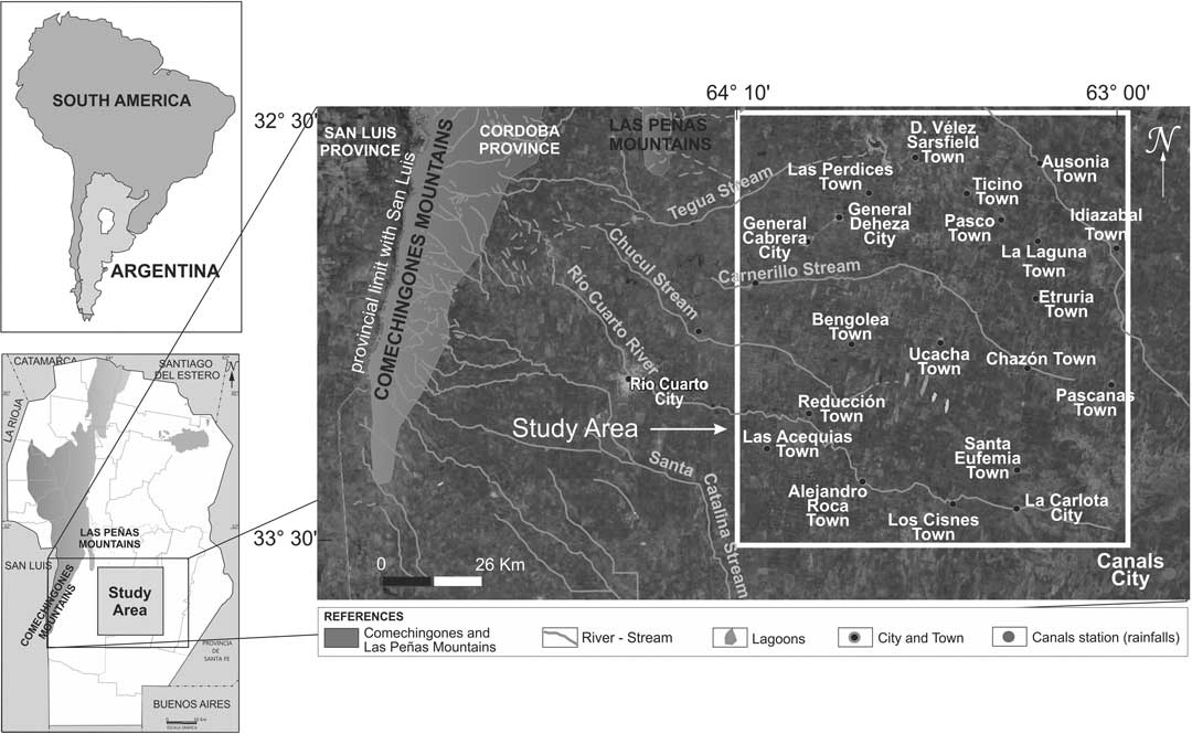
Figure 1 Location of the study area
MATERIALS AND METHODS
Standard geological and hydrogeological methodology was used for data collection. Groundwater levels were measured using water-level meters or manometers in the case of artesian wells. Next, hydraulic heads were calculated and piezometric maps were produced. Sediment samples were collected during drilling in selected sites to make textural studies. The results of grain-size analysis allowed us to estimate K values through empirical methods such as (a) the Sheelheim equation, to estimate K with the average particle size (Schafmeister Reference Schafmeister2006); (b) the Slichter equation, which bases the calculus on a particle size of 0.01–5 mm (Pérez et al. Reference Pérez, Tujchneider, Paris and D’Elia2014); and (c) the profile sieve percentage (PGP) (Pérez et al. Reference Pérez, Tujchneider, Paris and D’Elia2014), which uses triangular diagrams based on the model proposed by the US Department of Agriculture and considers both fine and coarse fractions. The results of these estimates were compared with K tables (Custodio and Llamas Reference Custodio and Llamas1996) and background data obtained in this region (Blarasin et al. Reference Blarasin, Cabrera and Matteoda2014). This information allows us to interpret the spatial configuration of different aquifer layers, to make correlations, and to estimate hydraulic aquifer parameters. In total, 71 groundwater samples were collected from unconfined and confined aquifers for chemical and isotopic analyses. The selected samples belong to wells with short screen lengths (<10 m) so that they are considered adequate for the interpretation of groundwater behavior at different depths, and preventing water mixture from different aquifers. Also, eight samples from streams and springs from the mountain and perimountain area were taken, in order to corroborate, mainly through the isotope information, the hypothesis of the potential recharge zones for the CAS.
During 2012–2015, 37 monthly composite rainfall samples were collected using a device located in the city of Canals, near the study area, following the International Atomic Energy Agency guidelines (IAEA/GNIP 2014). Rain samples were sent to for chemical and stable isotopes analyses, to know the input to the regional hydrological systems.
Field parameters, such as pH, electrical conductivity (EC), dissolved oxygen (DO), and temperature (T) were measured in situ. In the laboratory of the Geology Department of the National University of Rio Cuarto, the major ions (HCO3 –, SO4 2–, Cl–, Mg2+, Ca2+, Na+, K+) were determined using standard methods (APHA et al. 2005).
Stable isotope (2H and 18O) analyses were performed in the Instituto de Geocronología y Geología Isotópica (INGEIS-CONICET-UBA) using off-axis integrated cavity output spectroscopy (OICOS) (Lis et al. Reference Lis, Wassenaar and Hendry2008), with a DLT-100 liquid-water isotope analyzer from LGR Inc. Results were expressed in the conventional form, i.e. δ(‰), defined as
 $$\delta {\equals}1000{{R_{S} {\minus}R_{R} } \over {R_{R} }}$$
where R = isotope ratio 2H/1H or 18O/16O and δ = δ2H or δ18O, with isotopic deviation in ‰. R S denotes the sample and R R is the reference standard, which in the present case is V-SMOW (Gonfiantini Reference Gonfiantini1978). Uncertainties are ±1‰ for δ2H and ±0.3‰ for δ18O.
In addition, selected wells were sampled for 3H and 14C determination, to obtain representative values of different aquifer systems. Samples were prepared following the laboratory instructions and sent to the Environmental Isotope Laboratory of the University of Waterloo (Canada). Samples for 3H analysis were collected in 600-mL polyethylene bottles, while those for δ13C and 14C analyses were collected in 150-mL polyethylene bottles. All the samples were shipped in ice coolers. The 3H was determined by liquid scintillation counting (LSC) after electrolytic enrichment. The detection limit was of 0.8±0.3 tritium units (TU).14C and 13C samples were analyzed by an accelerator mass spectrometer (AMS).14C results are expressed as the percent of modern carbon (pMC) relative to the National Institute of Standards and Technology (NIST) SRM-4990C standard and normalized to δ13C =−25‰. The reference standard for δ13C is V-PDB (Craig Reference Craig1957) and the uncertainty is ±0.2‰. To correct 14C ages, the following methods were used: (a) the Tamers (Reference Tamers1975) method, which performs a chemical correction of the initial activity (14A); (b) the Pearson (Reference Pearson1965) method, which considers an isotopic correction of initial activity (14A); and (c) the Pearson-Gonfiantini method (Salem et al. Reference Salem, Visser, Dray and Gonfiantini1980), which involves chemical and isotope determinations.
HYDROGEOLOGY AND GROUNDWATER GEOCHEMISTRY
The area under study is situated in the middle of the Pampean plain (Figure 1), to the east of the Comechingones and Las Peñas Mountains. The regional tectonic scheme, an arrangement of blocks gradually descending eastwards, has influenced the sedimentation processes that gave rise to the different aquifers layers. This feature and the Quaternary climatic changes have affected the dynamic and geochemical processes of these groundwater systems over time.
The unconfined aquifer, with a thickness of almost 80–100 m, consists of fine Quaternary sediments and exhibits shallow groundwater levels. The base of the aquifer, formed by silty-clay sediments, has an average thickness of 20 m (Figure 2). The groundwater flow direction is NW-SE. Hydraulic characteristics are listed in Table 1. The aquifer geochemical pattern shows a salinity increase (EC from 777 to 15,600 µS/cm) along the flow path and the geochemical composition changes from sodium bicarbonate to sodium sulfate/chloride.

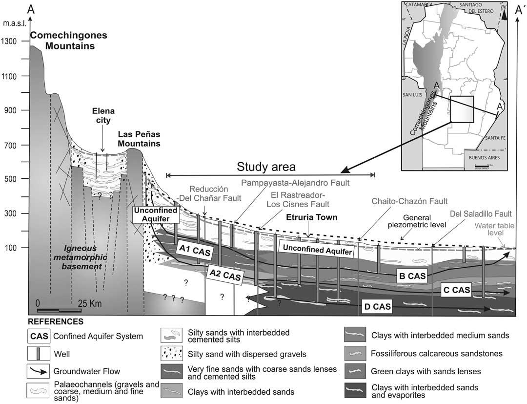
Figure 2 Regional hydrogeological A-A’ profile of southern Cordoba Province, Argentina (Blarasin et al. Reference Blarasin, Cabrera and Matteoda2014)
Table 1 Hydraulic parameters of the different aquifer systems.

The CASs, which show a lateral variable extension, are multilayered and formed by thin (4–6 m) sand-pebble lenses linked to Neogene–Pleistocene fluvial paleosystems or, in the eastern area, to sand marine layers (Blarasin et al. Reference Blarasin, Cabrera and Matteoda2014; Maldonado et al. Reference Maldonado, Cabrera, Blarasin, Dapeña and Panarello2015). These layers are situated at different depths, between 120 and 400 m, and are interlayered with thick aquitard or aquiclude silt-clay strata (40–80 m), which generate different confinement grades. Nodules of calcium carbonate can be observed in some layers. Hydraulic characteristics are listed in Table 1. Four principal CASs were identified: A1 and A2, B (not used for agricultural and urban activities, thus not considered for this study as a consequence of the scarce information), C, and D (Figure 2).
The A1 CAS is the shallowest system. The most permeable layers are mostly located between 100–120 and 190–230 m. A1 shows the less confinement grade according to the existing upper semipermeable materials. It extends from the western limit of the study area to the El Rastreador–Los Cisnes regional fault (Figure 2). The wells that pump groundwater from this system show piezometric levels between –22 and –3.5 m (beneath ground level), and the groundwater flow is west to east. The groundwater from the A1 CAS shows lower salinity (EC 823 to 4000 µS/cm; see Table 2) than the overlying unconfined aquifer. The A1 CAS has fresh to brackish sodium sulfate and sodium sulfate/bicarbonate water types in the N sector, where fine sediments predominate, and sodium bicarbonate water type in the S sector, where sand-gravel sediments dominate.
Table 2 Chemical and isotope (δ18O and δ2H) composition of confined aquifer systems.

The A2 CAS underlies A1 CAS and has a similar spatial distribution (Figure 2). It extends from 230–250 to 320–330 m depth. After the field measurements, it was interpreted that A2 is hydraulically connected with the C CAS; thus, the equipotential lines are presented in the same map (Figure 3). The wells that extract groundwater from this aquifer system are artesian, with piezometric levels that vary from +0.5 to +15 m (above ground level). This condition is related to the important confinement grade of the more permeable lenses of this system, which are interlayered with thick clay deposits. The groundwater flows from west to east, at different flow velocities (Table 1). The A2 CAS system has the freshest groundwater of the study area (EC 571 to 2400 µS/cm; see Table 2). The groundwater is sodium bicarbonate, sodium bicarbonate-sulfate, and sodium sulfate geochemical type. The low groundwater salinity in this system is linked to the coarse granulometry of the aquifer layers, which suggests lower water-sediments contact time. Moreover, because quartz grains prevail, the mineral weathering reactions decrease, thus lowering the transference of ions into solution.

Figure 3 Equipotential map of the A2 and C CAS systems
The C CAS is situated between 230 and 300 m depth (Figure 2 and 3). The wells that withdraw groundwater from this system are artesian, with piezometric levels that vary between +2 and +11 m. The more permeable layers are interbedded with thick greenish marine clay deposits. The groundwater flow in this system is NW-SE (Figure 3), with low hydraulic gradients and flow velocities (Table 1). In terms of salinity, the C CAS is characterized by EC values between 593 and 2690 μS/cm (Table 2), while the geochemical types are sodium bicarbonate, sodium sulfate, sodium bicarbonate-sulfate, and sodium bicarbonate-chloride. The main control on the groundwater geochemistry is the aquifer lithology, characterized by marine fine sands.
The D CAS is seen in the eastern part of the study area, located under the C system (Figure 2). It is the deepest system (320–400 m) and it shows the highest confinement grade as a result of thick overlying clay deposits. The wells that extract water from these layers are artesian, with piezometric levels that vary between +2 and +25 m. Some wells are artesian, despite overuse for more than 80 yr. The D CAS has a NW-SE groundwater flow direction, with low hydraulic gradients and low flow velocities (Table 1). This system returned the highest EC values (EC 1,121 to 3.600 µS/cm, see Table 2), and sodium sulfate-bicarbonate, sodium sulfate, sodium sulfate-chloride, and sodium chloride-sulfate groundwater types were identified. The high salinity values and the abundance of sulfate water types may be linked to the sediment composition, which includes some gypsum layers (Russo et al. Reference Russo, Ferello and Chebli1979).
ISOTOPE GEOCHEMISTRY
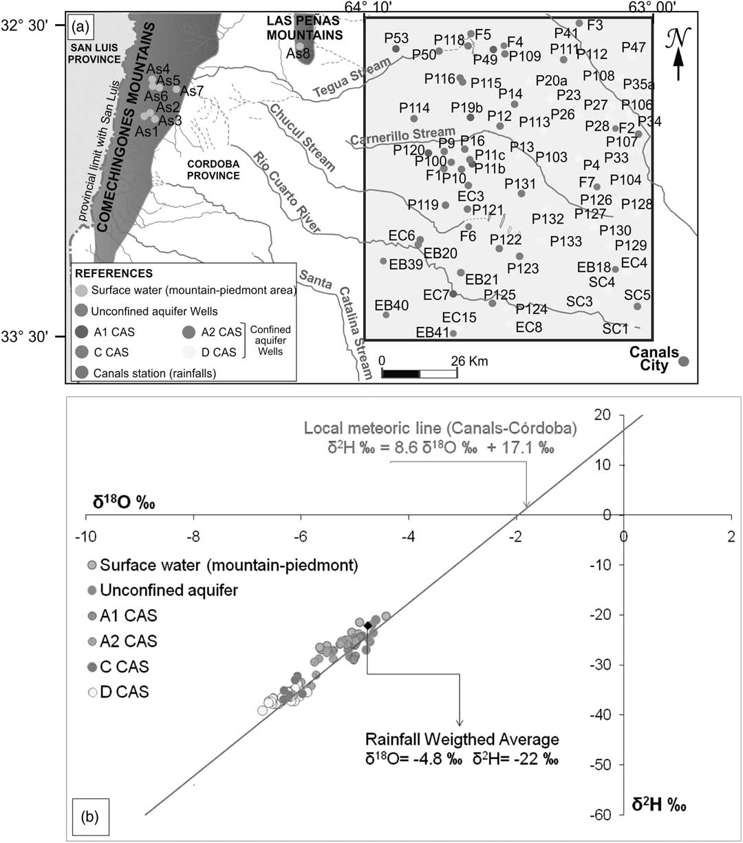
Precipitation isotopic values are aligned in a local meteoric line (Table 3, Figure 4), whose equation is δ2H =(8.6±0.2) δ18O + (17.1±1.2) ‰ obtained via orthogonal regression (IAEA 1992). The observed deuterium excess variations (d between +11‰ and +19‰) reveal different air mass origins, which probably produce rainfalls from recycled vapor related to the Low Level Jet (LLJ), the El Niño South Oscillation (ENSO) phenomenon, and the Intertropical Convergence Zone (ITZC) processes (Dapeña et al. Reference Dapeña, Panarello, Cerne, González and Sanchez-Coyllo2005; Gonzalez et al. Reference González, Dapeña, Cerne, Sanchez-Coyllo, Freitas, Silva Dias and Panarello2009; Cabrera et al. Reference Cabrera, Blarasin, Dapeña and Maldonado2013).

Figure 4 (a) Surface and groundwater sample locations; (b) δ2H vs. δ18O diagram for surface water and aquifer systems.
Table 3 δ18O and δ2H stable isotopic average values for each hydrological system.

The springs and the streams from the mountain area show an isotopic composition that suggests meteoric origin (Tables 2 and 3; Figure 4). These are more depleted than the eastern plain rainfalls (Canals station; Tables 2 and 3; Figure 4). This situation arises from a regional process in which the rains originate in a wet warm front that comes from the Atlantic Ocean (1000 km away), then suffer continental and altitude effects (Cabrera et al. Reference Cabrera, Blarasin, Dapeña and Maldonado2013; Giuliano Albo et al. Reference Giuliano Albo, Blarasin and Panarello2015).
Groundwater from the unconfined aquifer is characterized by an isotopic composition similar to the local rainfall (Tables 2 and 3; Figure 4), especially the rain that falls from September to February, the months during which the majority of aquifer recharge takes place (Cabrera et al. Reference Cabrera, Blarasin, Dapeña and Maldonado2013; Blarasin et al. Reference Blarasin, Cabrera and Matteoda2014).
It was observed that the A1 CAS has a similar isotopic composition to the unconfined aquifer and thus the local precipitation (Table 3, Figure 4). This situation allows us to correlate the hydraulic connection of each aquifer, taking into account the piezometric levels. Thus, the unconfined aquifer with a higher hydraulic head than A1 CAS would contribute water with a clear isotopic enriched signature from local precipitation, which would subsequently mix with depleted groundwater from the piedmont area.
The A2, C, and D CASs (Table 3, Figure 4) are more depleted in 2H and 18O than the unconfined aquifer and A1 CAS, suggesting a hydraulic disconnection with these systems. Moreover, these deep systems are more depleted than the surface water from the mountains and piedmont. This could be due to present recharge in higher areas or past recharge under a colder climate.
GROUNDWATER AGE ESTIMATION
Hydraulic Methods
The hydraulic age is based on Darcy’s law and takes into consideration a time water molecule trajectory (piston flow) from the recharge zone to a specific site where we need to know the age (Kazemi et al. Reference Kazemi, Lehr and Perrochet2006). In this way, using known values of the hydraulic gradients (i), effective porosity (ρ), and hydraulic conductivity (K), the age from young to very old groundwater may be calculated. In an aquifer with horizontal flow and no recharge along the flow line, such as a confined aquifer, the age of the groundwater at any point along the flow line equals the distance from the recharge area divided by the groundwater velocity, according to the following equation:
 $$Age{\equals}L\,/\,V$$
where L = trajectory longitude (m) and V = real velocity following Darcy’s law (m/d):
 $$V{\equals}{{k{\times}i} \over \rho }$$
where K = hydraulic conductivity (m/d), i = hydraulic gradient (%), and ρ = specific porosity (%).
Groundwater ages obtained using this methodology are shown in Table 4.
Table 4 3H, δ13C, and 14C results and ages reported from University of Waterloo laboratory and calculated ages with hydraulic methods and Pearson-Gonfiantini model (Salem et al. Reference Salem, Visser, Dray and Gonfiantini1980).

nd: not determined.
Stable Isotopes (2H and 18O)
As discussed, the various analyzed systems show differing isotopic composition, which suggests that recharge has occurred. In Figure 5, it can be observed that the CAS groundwater is depleted in the flow direction, a feature that agrees with each aquifer system depth. Taking into account the high depletion in 2H and 18O in the deepest CAS, especially the D CAS (Figure 4b), it thus may be interpreted that the groundwater is very old and would have been recharged in a previous geological epoch with colder climatic conditions than the present times.

Figure 5 δ18O values in the confined aquifers as a function of distance from the recharge zone. Groundwater flow is towards the east (i.e. towards the right).
Radioactive Isotopes (3H and 14C)
To estimate and interpret the groundwater ages of deep regional aquifers, 3H was measured in selected samples in the A1, A2, C, and D CASs, and compared with 3H concentration in precipitation, streams, and the unconfined aquifer, previously measured in the southern Cordoba Province (Cabrera et al. Reference Cabrera, Blarasin and Matteoda2010). The results given in Figure 6 and Table 4 suggest that these deep aquifers are not directly related to the present hydrological cycle.

Figure 6 3H concentration in the different water systems (Cabrera et al. Reference Cabrera, Blarasin and Matteoda2010; Maldonado et al. Reference Maldonado, Cabrera, Blarasin, Dapeña and Panarello2015)
When the 14C method is used for groundwater dating, some difficulties arise and ages must be corrected because of two reasons. The first is the difficulty in calculating the initial 14C concentration in the recharge precipitation due to fossil fuel burning and the influence of plants and soil. The second reason is the modification of 14C due to of geochemical reactions in the aquifers (such as the congruent dissolution of carbonate minerals, dissolution of carbonate or other calcium-containing minerals, the addition of dead carbon from other sources, etc.).
In the study area, the main geochemical process that would affect the 14C activity in the deep aquifers is the dissolution of carbonates. Although these aquifers have sulfated waters, they have moderate to high bicarbonate concentration (≥145 mg/L). Another process that would modify 14C activity is sulfate reduction, which can be discarded if it is taken into account that moderate oxic conditions exist at the studied depth (dissolved oxygen >2 mg/L) and that the groundwater contains moderate to high sulfate values.
As previously stated, to deal with these complexities, some methods for age corrections have been developed. The three models used adjust better for those samples with less 14C activity (D CAS, older samples). The Pearson (Reference Pearson1965) model gave dissimilar results, especially in those samples with high 14C activity. The Tamers (Reference Tamers1975) and Pearson-Gonfiantini (Salem et al. Reference Salem, Visser, Dray and Gonfiantini1980) models provided results more suitable for the hydrogeological model. In this paper, only the Pearson-Gonfiantini model results are presented. This equation includes both the chemical and isotopic composition of the water samples, and the results were in line with those obtained via hydraulic calculation:
 $$t(years){\equals}8267\ln \left( {{{C_{0} } \over C}} \right)$$
 $$C_{0} {\equals}\left[ {{{100\left( {\delta {}^{{13}}C_{m} {\minus}\delta {}^{{13}}C_{c} } \right)} \over {(\delta {}^{{13}}C_{{CO_{2} }} {\minus}\delta ^{{13}} C_{c} {\plus}{\epsilon})}}x\left( {1{\plus}{{2{\epsilon}} \over {1000}}} \right)} \right]$$
where C = 14C concentration in the sample, C 0 = initial 14C concentration, δ 13 C m = content of the carbonate species dissolved in the sample, δ 13 C C =content of the aquifer carbonate, δ 13 C CO2 = concentration of the soil CO2 at the time of recharge, and ε= fractionation factor between bicarbonate and CO2. The 14C ages obtained for the deep aquifers are presented in Table 4.
A2 CAS (EC6 and P115 samples)
Taking into account the δ13C values (Table 4), it may be considered that there was an important dissolution of carbonates, according to saturation indexes (SI) for calcite (−0.3), which would give an apparent groundwater aging; that is, groundwater would be younger. Figure 7 shows values that support this hypothesis. The ages obtained with the 14C method have high uncertainty levels but are similar to those obtained with the hydraulic method. The A2 CAS has younger groundwater than the deeper aquifers (C and D CAS), which is in line with the features of this aquifer system: the location near the mountains, its depth, and high groundwater gradient, and velocity.

Figure 7 14A vs. δ13C diagram of isochrons of the different confined aquifers systems.
C CAS (P131 sample)
Taking into account the laboratory values (Table 4), we obtained an age that also suggests dissolution of carbonates, but in a smaller proportion than in the samples described above. The obtained age is 10.8±3.0 ka BP, i.e. old groundwater. This result agrees with the location of the aquifer in the central sector of the plain, away from the recharge area, with low groundwater velocities, which favor water aging.
D CAS (P112, P126, SC4 samples)
These samples contain 14C lower values than the A2 and C CAS (Table 4). The low δ13C values, the small increase in alkalinity, and the SI for calcite (+0.1) suggest a near equilibrium situation (dissolution/precipitation), which may be showing that the apparent aging of groundwater is lower. Conversely, there is an evident gypsum dissolution (IS –1.1). That is, the low 14C values are likely to be the result of the radioactive decay itself, taking into account the similitude of corrected and uncorrected ages. Geochemical (sodium sulfate water) and isotope data (strongly depleted in 2H and 18O) show a gradual aging of groundwater in the direction of flow from recharge areas in the western mountains (outside the study area), which would confirm that these samples correspond to paleowaters.
The 14C ages obtained for the A2 and C CASs (up to 10.8±3.0 ka BP) and D CAS (up to 46.0±3.0 ka BP) allow us to conclude that groundwater was recharged during different geological periods.
CONCLUSIONS
The interpretations made from the stable isotope and 3H results, as well as with hydraulic calculations in the confined aquifer systems, suggested that the groundwater is old, and not related to the present hydrological cycle. It was also revealed that the age increased with depth and in the groundwater flow direction.
Ages estimated by hydraulic methods are general consistent with those of the 14C data. Taking into account the geochemical features, methanogenesis, and sulfate reduction, denitrification or anaerobic oxidation of organic matter would not be taking place into the confined aquifer systems. Therefore, it is assumed that the applied model takes into account dead C from carbonate dissolution as the main cause of decreased 14C activity, especially in the upper systems A2 and C.
The 14C ages obtained for the A2 and C CASs indicate waters recharged during the Holocene cold periods, between the Little Ice Age and the end of the Holocene Climatic Optimum, and during the last glaciation, respectively. Similarly, the D CAS comprises paleowaters that would have been recharged during the Pleistocene.
The proposed hydrogeological model demands attention in relation to the present mismanagement of CAS groundwater, especially if we take into account that these first results show long groundwater renewal times. In other words, groundwater resources must be carefully used and managed. It is thus necessary to collect more samples from each aquifer layer and to use other methods to improve the assessment of the internal dynamics of the groundwater system and the quantification of timescales associated with groundwater flow.
ACKNOWLEDGMENTS
This paper was supported by FONCyT-MINCyT Cordoba PID 35/08, UNRC and partially by IAEA Research Contract ARG: 17385; CRP F33020.