


1. Introduction
Membrane filters have a wide range of industrial and commercial applications. Water purification (Meng et al. Reference Meng, Chae, Drews, Kraume, Shin and Yang2009), beer clarification (der Sman et al. Reference der Sman, Vollebregt, Mepschen, Noordman and R.2012) and radioactive sludge removal (Ambashta & Sillanpää Reference Ambashta and Sillanpää2012), among many other processes, have all benefited from the use of filters capable of microfiltration or ultrafiltration. Increasing interest in studying filter design and filtering efficiency has resulted in many comprehensive review articles, such as that by Bowen & Jenner (Reference Bowen and Jenner1995), who provide a thorough overview of membrane separation technology, by Iritani (Reference Iritani2013), who surveys the various fouling mechanisms that operate during a membrane filtration process, and more recently by Chew, Kilduff & Belfort (Reference Chew, Kilduff and Belfort2020), who compiled experimental and modelling results on interfacial interactions and membrane fouling in tangential filtration. Other reviews survey different aspects of membrane filtration, such as filtration materials (Zahid et al. Reference Zahid, Rashid, Akram, Rehan and Razzaq2018), filtration techniques (Ersahin et al. Reference Ersahin, Ozgun, Dereli, Ozturk, Roest and van Lier2012) and applications to chemical waste treatment (Daniel et al. Reference Daniel, Schonewill, Shimskey and Peterson2010).
There are three typical microporous membrane filtration modes – tangential, dead-end filtration and direct flow – with respective merits and shortcomings. The difference between the first two modes of filtration is that, in the former case, the fluid flow is parallel to the membrane surface whereas flow in the latter case is perpendicular to the membrane surface Chew et al. (Reference Chew, Kilduff and Belfort2020). Under the same transmembrane pressure, tangential filtration also requires more energy to obtain the same throughput: not all solute passes through the membrane; some recycles back to the feed. By contrast, in dead-end filtration, all energy goes into forcing the solute through the membrane (the interested reader is referred to Daniel et al. (Reference Daniel, Schonewill, Shimskey and Peterson2010) for a more detailed discussion on the relative merits of these two processes). Direct flow is similar to cross-flow but with one end of the central channel closed off by a cap and both sides of the channel operating as membrane filters (Collum Reference Collum2017).
In all filtration modes, particles within the fluid interact with the membrane material physically or chemically, leading to membrane fouling, the process by which foulants deposit on the membrane surface or within the pores. Membrane fouling occurs by three principal mechanisms: (1) adsorption, an accretion process in which small particles adhere to the pore walls and thus shrink the effective radius of the pore; (2) blocking, a discrete process in which particles larger than pores cover (partially or completely) the entrance of a pore; and (3) caking, in which an additional layer of porous medium, composed of the particles carried by the flow, forms on top of the membrane surface (this occurs particularly in the later stages of a membrane filtration process). These fouling modes have been studied via experiments and numerical simulations, both in isolation and with multiple modes operating simultaneously, by many researchers with a goal of developing predictive modelling; see for example the works of Polyakov (Reference Polyakov2008) and Bolton, Boesch & Lazzara (Reference Bolton, Boesch and Lazzara2006a) on adsorption, Hwang, Liao & Tung (Reference Hwang, Liao and Tung2007) on blocking, Daniel et al. (Reference Daniel, Billing, Russell, Shimskey, Smith and Peterson2011) on caking and Bacchin et al. (Reference Bacchin, Derekx, Veyret, Glucina and Moulin2014), Bolton, LaCasse & Kuriyel (Reference Bolton, LaCasse and Kuriyel2006b), Ho & Zydney (Reference Ho and Zydney2000) and Sanaei et al. (Reference Sanaei, Richardson, Witelski and Cummings2016) for multiple simultaneous modes. In the present work, we consider dead-end filtration as the primary type of filtration and adsorption as the dominant fouling mechanism. This approach facilitates a simpler system than would be obtained by considering all fouling modes, allowing us to focus on gaining insight into the effects of pore connectivity. We defer the study of multiple fouling modes in a pore-network model to a future work.
There is considerable industrial interest in designing and manufacturing layered filters that allow for fine control of particle removal while maintaining a reasonable filter lifetime. Such filters typically have pore size that decreases from one layer to the next (in the direction of flow; see figure 1a). In this way, pore closure occurs more uniformly throughout the filter, since fouling begins at the upstream side of the membrane, and thus the fouling rate is a decreasing function of depth through the membrane (as is the concentration of particles in the feed). Such layered structures may incorporate varying degrees of connectivity between pores in different layers, seen in figure 1(b).

Figure 1. Magnified membrane images showing (a) gradation of pores sizes through membrane depth, and in-plane inhomogeneity of pore sizes (Li Reference Li2009), (b) connectivity and junction layer (Yang et al. Reference Yang, Park, Yoon, Ree, Jang and Kim2008) and (c) pore-size distributions (Souza & Quadri Reference Souza and Quadri2013).
The literature on the influence of membrane morphology (pore structure and connectivity) on filtration efficiency is too large to provide a comprehensive review (but see, for example, Ho & Zydney Reference Ho and Zydney1999; Kanani et al. Reference Kanani, Fissell, Roy, Dubnisheva, Fleischman and Zydney2010; Zydney Reference Zydney, Oyama and Stagg-Williams2011; Griffiths, Kumar & Stewart Reference Griffiths, Kumar and Stewart2014, Reference Griffiths, Kumar and Stewart2016; Dalwadi, Griffiths & Bruna Reference Dalwadi, Griffiths and Bruna2015). Here we briefly outline the most relevant work that provides the primary motivation for our paper. The starting point for our modelling is the work of Sanaei & Cummings (Reference Sanaei and Cummings2018), who introduced a simple bifurcating-pore model to capture some of the layering features described above. In that paper, adsorption is the sole fouling mechanism: small particles are transported through a network of initially circularly cylindrical pores, and deposited on the pore walls. The particle concentration in the flow decreases as the pore network is traversed, with the goal that it reaches a sufficiently low level by the time the flow exits the filter. While the bifurcations model inter-layer pore connectivity, there is no additional intra-layer connectivity (see figure 1b) to allow interactions between pores in the same layer. Griffiths et al. (Reference Griffiths, Kumar and Stewart2016) accounted for such a feature by means of an ad hoc connectivity parameter, which can be tuned to adjust the degree of communication (allowed flux) between pores that occupy the same layer. An important new feature of our present work is the incorporation of inter-layer junctions with concentration- and pressure-equalizing capabilities that influence membrane performance metrics (detailed in § 2.3). Furthermore, neither Sanaei & Cummings (Reference Sanaei and Cummings2018) nor Griffiths et al. (Reference Griffiths, Kumar and Stewart2016) consider pore-size variation within individual layers. Such pore-size variation (which we term intra-layer heterogeneity, or heterogeneity in short) is another novel feature of the present work: it is inevitable due to imperfect manufacturing and, as we shall see, it may have non-intuitive implications for membrane performance.
In this paper, we introduce simple models of membrane pore networks that incorporate both intra-layer connectivity and heterogeneity. Our goal is to study and explain the effects of membrane connectivity and investigate the influence of pore-size variations introduced by manufacturing defects. The paper is arranged as follows. In § 2, we describe a mathematical model for the flow inside a membrane with homogeneous intra-layer structure and its heterogeneous analogue; in § 3, we give appropriate scalings and non-dimensionalizations for these models; and in § 4, we present results and discuss their implications and limitations. Lastly in § 5, we present our conclusions and discuss several ideas for future extensions of this work.
2. Mathematical modelling
In this paper, we consider a planar membrane filter whose top (upstream) surface resides in the  $Y$–
$Y$– $Z$ plane, as shown in figure 2(a). The flow is (at least initially) assumed to be entirely unidirectional, in the positive
  $X$ direction. Furthermore, the membrane pore structure is assumed homogeneous in the
  $Y$–
$Y$– $Z$ plane, but is allowed to vary internally along the
  $X$ axis, thereby imparting depth-dependent permeability. Throughout this work, uppercase symbols denote dimensional quantities, while lowercase symbols are dimensionless (see § 3).

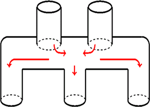
Figure 2. Illustration of a connected, branched-pore membrane and volumetric flow rate balance at pore junctions. (a) A three-layer ( $m=3$) pore network with unit cell area
  $(2W)^2$. (b) Schematic bifurcation of a single pore (left) and two pores merging into one (right), homogeneous in both cases. In the former case
  $Q_1=2 Q_2$ and in the latter
  $2Q_1=Q_2$, by mass conservation.
We assume that a membrane consists of units that repeat periodically in the  $Y$–
$Y$– $Z$ plane of the membrane in a square lattice pattern, with period
  $2W$. Globally, we assume incompressible unidirectional Darcy flow (Probstein Reference Probstein1994) across the porous medium, in which the superficial Darcy velocity,
  $\boldsymbol {U}=(U (X,T),0,0)$, is directly proportional to the pressure gradient:
 \begin{equation} U= -\frac{K (X,T)}{\mu} \frac{\partial P}{\partial X} , \quad \frac{\partial U}{\partial X} = 0, \quad 0\leq X \leq D, \end{equation}
where  $K(X,T)$ is the permeability at depth
  $X$ and
  $D$ is the thickness of the entire membrane. A pressure difference across the membrane acts as the driving force for fluid flow, and hence the following boundary conditions are imposed:
 \begin{equation} P(0,T) = P_0, \quad P(D,T) = 0. \end{equation}
Locally, the membrane's pore network is modelled as a composition of cylindrical tubes, of circular cross-section. The Hagen–Poiseuille model, which provides the local permeability  $K(X,T)$ in terms of the local pore radii, is a suitable framework for this structure.
2.1. Homogeneous model
We now present our connected pore model, first in the simplest homogeneous case in which all pores within a given layer are identical. To incorporate intra-layer connectivity, here referred to simply as connectivity, we require that at least two pores in the  $i$th layer connect in the
  $(i+1)$th layer; see figure 2(a) for an example of a two-inlet connected membrane. In this example, the basic period-unit has a top layer that consists of two inlet pores (identical tubes of length
  $D_1$ and radius
  $A_1$) on the upstream membrane surface. Flow from these two pores enters the first inter-layer region, where mixing occurs. The flow then enters the second layer of the membrane, consisting of three identical tubular pores of length
  $D_2$ and radius
  $A_2$, which exit into the second inter-layer region, where mixing again occurs. This structure repeats, so that the
  $i$th layer contains
  $i+1$ pores, with mixing in each inter-layer region.
More generally, for a membrane with  $m$ layers and
  $\nu _i$ pores in layer
  $i$, we assume that the inter-layer junction regions are short enough to have negligible resistance so that the pressure drop between the exit of pores in layer
  $i$ and the entrance of pores in layer
  $i+1$ is negligible (also see Sanaei & Cummings Reference Sanaei and Cummings2018; Chang & Roper Reference Chang and Roper2019). Because all pores in the
  $i$th layer have the same initial radius and length, they consequently experience the same local volumetric flow rate,
  $Q_i$. Incompressibility (mass conservation) conditions for the fluid yield
 \begin{equation} \frac{\partial Q_i}{\partial X} = 0, \quad 1 \leq i \leq m, \end{equation}
where  $Q_i$ through any pore in the
  $i$th layer can be related to the corresponding cross-sectionally averaged pore velocity
  $\overline {U}_{\mathrm{p},i}$:
 \begin{equation} Q_{i} = {\rm \pi}A_{i}^2 \overline{U}_{\mathrm{p},i}, \quad X_{i-1} \leq X \leq X_i, \quad X_i=\sum_{j=0}^{i} D_j,\quad D_0 = 0, \quad 1 \leq i \leq m, \end{equation}
with  $A_{i} = A_{i}(X,T)$ and
  $D_i$ the radius and the length of each pore in the
  $i$th layer, respectively. The chosen cylindrical pore geometry allows us to calculate
  $Q_i$ using the Hagen–Poiseuille equation:
 \begin{equation} Q_{i} = -\frac{(P_{i} - P_{i-1})}{\mu R_i}, \quad R_i = \frac{8}{{\rm \pi} } \int_{X_{i-1}}^{X_{i}} \frac{\textrm{d} X}{A_i^4(X,T)}, \end{equation}
where  $P_i$ is the pressure at the exit and
  $R_i$ the total resistance, for each pore in the
  $i$th layer. By continuity, we have
 \begin{equation} Q\equiv (2W)^{2}U=\nu_i Q_i, \quad 1 \leq i \leq m, \end{equation}
where  $Q$ is the global volumetric flow rate across the membrane,
  $U$ the global superficial Darcy velocity and
  $\nu _i$ the number of pores in the
  $i$th layer, which will vary depending on the exact pore architecture chosen (in the example of figure 2a,
  $\nu _i = i+1$). Volumetric flow rate through the
  $i$th layer in the membrane,
  $\nu _{i} Q_{i}$, can then be related to the local pore velocity,
  $\overline {U}_{\mathrm{p},i}$, under the assumption that the pressure gradient is uniform across each layer (an assumption implicit in (2.5a,b)). For the case that the imposed pressure is the same at each inlet, this condition becomes equivalent to stating that at each junction the flow rate ‘splits’ evenly – i.e. the fluid mass is divided at each junction according to the number of pores.
Note that (2.5a,b) and (2.6) together yield  $m$ equations for the global superficial Darcy velocity,
  $U$, and the inter-layer pressures,
  $P_i$. Solving successively for
  $P_i$ gives
 \begin{equation} (2W)^2 U = \frac{P_0}{\mu R}, \quad R = \sum_{i=1}^{m} \frac{R_i}{\nu_i}. \end{equation}
The above equation for  $R$ describes the net resistance of the membrane. To compare and contrast with the single-inlet non-connected bifurcating pore model presented by Sanaei & Cummings (Reference Sanaei and Cummings2018) (where
  $\nu _i = 2^{i-1}$), we will consider single-inlet and two-inlet connected pore models, with linear growth in the number of pores through each layer. In these two cases,
  $\nu _i=i$ and
  $i+1$, respectively, in (2.6).
2.1.1. Particle transport and fouling
The model described above constitutes Darcy flow through the membrane with the specified pore architecture, and we now develop the model for the transport and deposition of foulants. In this paper, we consider membrane fouling due to adsorption (also known as standard blocking) only, as we intend to study the effect of different pore architectures rather than the complexities of multiple fouling mechanisms. Adsorptive fouling is the process of small particles adhering to the walls of the pores, thereby shrinking the pore radius, and is dominant in many applications. To model this, within each pore we follow Sanaei & Cummings (Reference Sanaei and Cummings2017), where an asymptotic analysis of the advection–diffusion equation governing particle transport down pores is carried out, revealing that (in a certain distinguished Péclet number limit) diffusion dominates in the radial direction, leading to particle concentration that is approximately uniform across the pore cross-section, while variation in concentration along the length of the pore is governed by an advection equation:
 \begin{equation} \overline{U}_{\mathrm{p},i}\frac{\partial C}{\partial X} = -\Lambda \frac{C}{A_i}, \quad X_{i-1} \leq X \leq X_i, \quad 1 \leq i \leq m. \end{equation}
Here,  $A_i(X,T)$ is the pore radius,
  $C(X,T)$ is the local concentration of adsorption foulants carried by the flow in the membrane,
  $\overline {U}_{\mathrm{p},i}$ is the cross-sectionally averaged pore velocity (see (2.4a–d)) and
  $\Lambda$ is a parameter (with dimensions of velocity) that captures the physical attraction between particles and pore walls. This equation is solved subject to a specified particle concentration at the upstream surface:
 \begin{equation} C(0,T)=C_0.\end{equation}
In real filters, it is desirable to have membrane outlet concentration  $C(D,T)$ significantly smaller than
  $C_0$ and therefore
  $C$ must vary spatially in
  $X$. In fact, according to (2.8),
  $C$ changes continuously through the depth of the filter since the concentration at the downstream surface of a given layer must match with that at the upstream surface of the next. At the same time, since the pore radius
  $A_i$ jumps in value between layers (by design), we must in general expect
  $\partial C/\partial X$ to be discontinuous at layer junctions. In the next subsection we will justify and carry out a coarse-grained discretization of (2.8), which leads us to a simple approximate model for the particle concentration within each layer.
The rate of pore radius shrinkage in each layer is proposed to be proportional to the local concentration of particles. The assumption underlying our deposition law, similar to that in Sanaei & Cummings (Reference Sanaei and Cummings2018), is that (at a given location  $X$ in the pore) in a time increment
  $\delta T$ the change in pore area,
  $2{\rm \pi} A_i \delta A_i$, is proportional to the void fraction of particles locally (
 $\alpha C$, where
  $\alpha$ is an effective particle volume), the deposition coefficient
  $\Lambda$ and the pore circumference available for particles to stick to:
 \begin{gather} \frac{\partial\left({\rm \pi} A_{i}^2\right)}{\partial T} = 2{\rm \pi} A_{i}\frac{\partial A_{i}}{\partial T}= -\Lambda \alpha C \left(2{\rm \pi} A_{i}\right) \iff \frac{\partial A_i}{\partial T} = -\Lambda\alpha C, \end{gather}
 \begin{gather}X_{i-1} \leq X \leq X_i, \quad A_{i}(0) = A_{i0}, \quad 1\leq i \leq m. \end{gather}
2.1.2. Spatial discretization (coarse-grained model)
The system of partial differential equations (PDEs) described by (2.8)–(2.11a,b) must be solved numerically. Sanaei & Cummings (Reference Sanaei and Cummings2018) did not consider pore-size variation within layers and were able to solve the full system of PDEs as presented above to obtain results. In our case, our later simulations for heterogeneous membranes require simulations where the radii of pores in the same layer are randomly assigned, and a large number of simulations is needed to obtain reliable statistics representative of an entire membrane, which is numerically expensive. Therefore, we propose instead a coarse-grained discretization of the model (2.8)–(2.11a,b) in which we solve for quantities  $A_i$ and
  $C_i$ that represent approximations to pore radius and particle concentration within layer
  $i$, respectively.
If one assumes that the layers are sufficiently numerous that the particle concentration does not change appreciably across a single layer (corresponding to an assumption that  $32\Lambda \mu D^2/({\rm \pi} m P_0 W^3)\ll 1$; see (2.8)) then such a coarse-grained approximation should be reasonable. The particle concentration can then be approximated by a piecewise (spatially) constant function,
  $C_i(T)$, changing in value from one layer to the next. We note that if
  $C_i(T)$ is assumed independent of
  $X$ across a given layer
  $i$, then consistency requires that the pore radii must also be independent of
  $X$ in layer
  $i$,
$i$,  $A_i(T)$, and therefore shrink uniformly within a given layer over time. The particle concentration within the first layer is taken to be
  $C_0$, the concentration in the feed, making a jump to the value
  $C_1$ at the boundary between first and second layers. More generally, the concentrations within each layer are taken to satisfy
 \begin{equation} \overline{U}_{\mathrm{p},i} \frac{C_{i}-C_{i-1}}{D_i}=-\Lambda \frac{C_{i}}{A_{i}}, \quad 1\leq i \leq m, \end{equation}
(replacing (2.8)) with  $C_0$ specified as in (2.9). This equation allows the particle concentration
  $C_{i}$ in each pore in layer
  $i$ to be expressed in terms of the concentration in the previous layer as
 \begin{equation} C_{i}=\frac{\overline{U}_{\mathrm{p},i}C_{i-1}}{\overline{U}_{\mathrm{p},i}+\Lambda D_i/A_{i}}, \quad 1\leq i \leq m. \end{equation}
For the pore radius we propose
 \begin{equation} \frac{\partial A_i}{\partial T} = -\Lambda\alpha C_{i-1}, \quad 1\leq i \leq m, \end{equation}
as the coarse-grained discretization of (2.11a,b). Note the shift of index on the right-hand side: since particle deposition occurs first at the upstream side of pores, it is the concentration at pore inlets that dominates the fouling and pore closure, hence (we have confirmed) using the upstream value  $C_{i-1}$ gives more accurate results than using either the downstream value
  $C_{i}$ or an average
  $(C_i+C_{i-1})/2$. At the same time local resistance
  $R_i$, previously defined in (2.5a,b), reduces to
 \begin{equation} R_i = \frac{8 D_i}{{\rm \pi} A^{4}_{i}}, \end{equation}
since each pore in the  $i$th layer has length
  $D_i$.
To check the accuracy of our coarse-grained model we carried out simulations, and compared with solutions to the full PDE model over a range of geometric and material parameters. In all simulations presented in this paper we use parameter values such that the coarse-grained model gives less than 5 % error when compared with fully converged solutions to the PDE model (see appendix A for more details of how this determination of accuracy was made).
2.2. Heterogeneous model
Until now, we have focused on a homogeneous model in which all pores within a given layer of the membrane are identical. Now, we turn our attention to heterogeneous connected pore membranes in which the initial pore sizes within a given layer may vary. Consequently, pores in the  $i$th layer do not necessarily experience identical volumetric flow rates. Similar to (2.4a–d), the net volumetric flow rate through pores is given by
 \begin{equation} Q_{ij} = {\rm \pi}A_{ij}^2\overline{U}_{\mathrm{p},ij}, \quad 1\leq i\leq m, \ 1\leq j \leq \nu_i, \end{equation}
where  $A_{ij}$ and
  $\overline {U}_{\mathrm{p},ij}$ are the radius of the
  $j$th pore in the
  $i$th layer and the cross-sectionally averaged pore velocity, respectively. By balancing the flow rates through a mass-conservation argument (cf. figure 2b), we allow for non-uniform splitting of the flow at each junction. A general representation of this model in terms of the global superficial Darcy velocity (and global volumetric flow rate
  $Q$) is given by
 \begin{equation} Q = (2W)^2U = \sum_{j=1}^{\nu_i} Q_ {ij}, \quad 1 \leq i \leq m. \end{equation}
Again, the junction regions are assumed to be of sufficiently low resistance that pressure is spatially uniform within them, with perfect mixing of the flow in these regions so that the concentration  $C$ of suspended particles is spatially uniform. Similarly to (2.5a,b),
  $Q_{ij}$ through and resistance
  $R_{ij}$ of the
  $j$th pore in layer
  $i$ become
 \begin{equation} Q_{ij} = -\frac{(P_{i} - P_{i-1})}{\mu R_{ij}}, \quad R_{ij} = \frac{8}{{\rm \pi} }\int_{X_{i-1}}^{X_{i}} \frac{\textrm{d} X}{ A_{ij}^4(X,T)}, \quad 1 \leq i \leq m, \ 1 \leq j \leq \nu_i. \end{equation}
By continuity,  $Q$ and
  $\sum ^{\nu _{i}}_{j=1}Q_{ij}$ must be equal. In view of this, (2.17) and (2.18a,b) lead to
  $m$ equations which, when solved successively for
  $P_i$, yield (cf. (2.7a,b))
 \begin{equation} Q=(2W)^2 U = \frac{P_0}{\mu R}, \end{equation}
where  $R$ is the total resistance of the membrane, now given by
 \begin{equation} R = \sum_{i=1}^{m}\ \left(\sum_{j=1}^{\nu_i}\frac{1}{R_{ij}}\right)^{-1}. \end{equation}
Comparing this expression with resistors in an electrical circuit, one can see the  $\nu _i$ pores in the
  $i$th layer are analogous to resistors in a parallel circuit, while the total resistance of each layer is summed as for resistors in series. Using (2.17) and (2.19) to isolate
  $P_i - P_{i-1}$ in (2.18a,b), we arrive at an explicit expression for
  $Q_{ij}$:
 \begin{equation} Q_{ij} = {\rm \pi}A_{ij}^{2}\overline{U}_{\mathrm{p},ij} = \frac{P_0}{\mu R\left( R_{ij} \displaystyle\sum_{j=1}^{\nu_i} \frac{1}{R_{ij}}\right)}, \quad 1 \leq i \leq m, \ 1 \leq j \leq \nu_i. \end{equation}
2.2.1. Particle transport and fouling
Fouling and foulant transport for the heterogeneous scenario are governed similarly to the homogeneous case, but here particle concentrations at the outlets of pores in a given layer are not the same because the pores have differing initial radii, which leads to different fouling behaviour. Continuity of concentration is therefore not automatic in the inter-layer regions, and we need to invoke our perfect mixing assumption in order to close the model. The transport equations now read
 \begin{equation} \overline{U}_{\mathrm{p},ij} \frac{\partial C_{ij}}{\partial X}=- \Lambda \frac{C_{ij}}{A_{ij}}, \quad X_{i-1} \leq X\leq X_i , \ 1\leq i \leq m, \ 1 \leq j \leq \nu_i, \end{equation}
where  $C_{ij}$ is the cross-sectionally averaged concentration of foulants in the
  $j$th pore of layer
  $i$. The initial condition is
 \begin{equation} C_{01}(T)=C_0.\end{equation}
With our perfect mixing assumption the uniform particle concentration,  $C_{i,mix}$, in the junction region below the
  $i$th layer satisfies
 \begin{equation} C_{i,mix} := \frac{\displaystyle\sum_{j=1}^{\nu_i} Q_{ij}C_{ij}}{\displaystyle\sum_{j=1}^{\nu_i} Q_{ij}}, \quad 1 \leq i \leq m. \end{equation}
With  $C_{ij}$ calculated from (2.22),
  $C_{i,mix}$ then provides the boundary (upstream) condition to calculate
  $C_{i+1,j}$ (see figure 3).

Figure 3. Schematic of a connected branching-pore membrane with  $m=2$ layers, pressure drop
  $P_0$ and upstream particle concentration
  $C_0$. Flow is assumed to be entirely in the
  $X$ direction.
The rate of change in pore radius is again determined as in (2.11a,b). The only modification is the introduction of double indices, so that the rate of change of radius of the  $j$th pore in layer
  $i$ is given by
 \begin{equation} \frac{\partial A_{ij}}{\partial T}=-\Lambda \alpha C_{i-1,j}, \quad 1\leq i \leq m, \ 1\le j \le \nu_i, \end{equation}
with the initial pore radii specified:  $A_{ij}(0)=A_{ij0}$. Note that this general heterogeneous model reduces to the homogeneous model when all pores in a given layer are identical.
2.2.2. Spatial discretization (coarse-grained model)
We modify (2.12) according to the concentration rebalance introduced in (2.24), replacing  $C_{i-1}$ by the appropriate upstream value
  $C_{i-1,{mix}}$. The heterogeneous analogue of (2.13) then becomes
 \begin{equation} C_{ij}=\frac{\overline{U}_{\mathrm{p},ij}C_{i-1,{mix}}}{\overline{U}_{\mathrm{p},ij}+\Lambda D_i/A_{ij}}, \quad C_{0,{mix}}=C_{0}, \ 1\leq i \leq m, \ 1\le j \le \nu_i, \end{equation}
and the radius of pore  $j$ in the
  $i$th layer evolves at the following rate:
 \begin{equation} \frac{\partial A_{ij}}{\partial T}=-\Lambda \alpha C_{i-1,{mix}}, \quad 1\leq i \leq m, \ 1\le j \le \nu_i. \end{equation}
Similar to (2.15),  $R_{ij}$, the total resistance of the
  $j$th pore in the
  $i$th layer, defined in (2.18a,b), now reduces to
 \begin{equation} R_{ij} = \frac{8 D_i}{{\rm \pi} A^{4}_{ij}}. \end{equation}
2.3. Measures of performance
There are several primary measures of membrane performance used in applications. First, volumetric throughput (referred to simply as throughput henceforth), which represents the total cumulative volume of filtered fluid (filtrate) collected at the outlet of the filter by time  $T$, is defined as the time integral of the global volumetric flow rate
  $Q$, i.e.
 \begin{equation} V(T) = \int_0^T Q(T') \, \textrm{d} T'. \end{equation}
Flow rate  $Q$ is often plotted against throughput
  $V$ to illustrate the relative efficiency of the filter. A desirable performance would be represented by a relatively uniform
  $Q$ during most of the filtration, during which significant throughput is achieved, followed by a sharp drop in
  $Q$ towards the end of the filter's lifetime when fouling is severe.
Another important performance metric is the concentration of foulants at the outlet of the membrane,  $C_{m}(T)\equiv C_{m,{mix}}(T)$ (see (2.24)). Calculating these performance measures using our model, our simulations will allow us to study the dynamics of filtration, infer dependence on material and geometric parameters and ultimately infer the most efficient filtration scenarios.
3. Scaling and non-dimensionalization
3.1. Homogeneous model
The model presented in § 2.1 is non-dimensionalized using the following scalings:
 \begin{equation} \left. \begin{array}{c@{}} P_i = P_0p_i, \quad (X,D_i) = D(x,d_i), \quad C_i = C_0c_i, \quad A_i = Wa_i, \\ (U,\overline{U}_{\mathrm{p},i}) = \dfrac{{\rm \pi} W^2 P_0}{32\mu D\hat{r}_0}(u, \bar{u}_{\mathrm{p},i}), \quad T = \dfrac{W}{\Lambda \alpha C_0}t, \end{array}\right\} \end{equation}
where the physical scaling quantities are defined in table 1 (with the exception of  $\hat {r}_0$, a representative value of the membrane resistance, which is defined below). After applying the boundary conditions for pressure,
 \begin{equation} p_0(t) = 1,\quad p_m(0) = 0, \end{equation}
the resulting dimensionless model for  $u(t)$,
  $\bar{u}_{\mathrm{p},i}(t)$,
  $r(t)$,
  $a_i(t)$ and
  $c_i(t)$ (global Darcy velocity, cross-sectionally averaged pore velocity, total membrane resistance, radius of pores in the
  $i$th layer and particle concentration in the
  $i$th pore, respectively) is
 \begin{gather} r = \frac{1}{\hat{r}_0} \sum^m_{i=1}\frac{d_i}{\nu_i a_i^4},\end{gather}
 \begin{gather} u = \frac{1}{r}, \quad u = \frac{\nu_i}{4}{\rm \pi} a_{i}^2\bar{u}_{\mathrm{p},i},\end{gather}
 \begin{gather} c_i = \frac{\bar{u}_{\mathrm{p},i} \, c_{i-1}}{\bar{u}_{\mathrm{p},i}+\lambda d_i/a_i}, \quad \lambda = \frac{32 \mu D^2 \hat{r}_0}{{\rm \pi} P_0 W^3}\Lambda, \quad \frac{\partial a_i}{\partial t} = -c_{i-1}, \quad 1\leq i \leq m.\end{gather}
Here  $\hat {r}_0$ is chosen from a typical value (
 $\hat {r}_0 = 15\,000$ in most of the cases we analyse; see § 4 for more details) of
 \begin{equation} \hat{r}\left(0 \right) = \sum_{i=1}^m \frac{d_i}{\nu_i a_i^4\left(0 \right)}, \end{equation}
to ensure  $r$ and
  $u$ take order-one values (at least initially), and
  $\lambda$ is a dimensionless deposition parameter that describes the competition between the affinity of the foulant particles for the membrane material and the downstream flow (which depends on physical quantities such as viscosity
  $\mu$, transmembrane pressure
  $P_0$, etc.). Note that this choice of scaling (rather than simply scaling on the membrane's initial resistance in all cases) enables us to make direct comparisons of membranes with different initial resistances.
Table 1. Key nomenclature used throughout this work. Uppercase symbols denote dimensional quantities; lowercase are dimensionless.

We also define dimensionless volumetric flow rate  $u(t)$ and throughput
  $v(t)$:
 \begin{equation} Q = \frac{{\rm \pi} W^4 P_0}{8\mu D\hat{r}_0}u, \quad V = \frac{\left(2W\right)^2 D}{\alpha C_{0}}v, \quad v(t) = \frac{1}{\lambda}\int^t_0 u\left(t^{\prime}\right)\textrm{d} t^{\prime}; \end{equation}
see the definitions of dimensional global volumetric flow rate  $Q$ (2.19) and throughput
  $V$ (2.29). These quantities are often compared when studying membrane performance. We make comparisons between real membranes with variations only in
  $\Lambda$ while all other physical parameters (e.g.
  $\mu , D, P_0, W$) are held fixed. The resulting variations in
  $\lambda$ are directly reflected in the time scale in (3.1), but no other scalings are affected. The factor of
  $1/\lambda$ in
  $v$ then emerges naturally after using the scales of
  $Q$,
$Q$,  $V$ and
  $T$ in the definition of throughput (2.29).
Non-dimensionalized boundary and initial conditions are given by
 \begin{equation} c_0(t) = 1, \quad a_i(0) = a_{i0}, \end{equation}
with  $a_{i0}$ specified for
  $1 \leq i \leq m$. This closes the system described by (3.3)–(3.5).
3.2. Heterogeneous model
The heterogeneous model is also non-dimensionalized using the scalings of (3.1). The relevant non-dimensional equations are then
 \begin{gather} r = \frac{1}{\hat{r}_0}\sum_{i=1}^m d_i \, \left(\sum_{j=1}^{\nu_i} a_{ij}^4\right)^{-1}, \end{gather}
 \begin{gather}u = \frac{1}{r}, \quad \bar{u}_{\mathrm{p},ij} = \frac{4}{{\rm \pi} } a_{ij}^2 \frac{1}{ r\left(\displaystyle\sum_{j=1}^{\nu_i}a_{ij}^4\right)^{-1}}, \end{gather}
 \begin{gather}c_{ij} = \frac{\bar{u}_{\mathrm{p},ij} \, c_{i-1,{mix}}}{\bar{u}_{\mathrm{p},ij}+\lambda d_i/a_{ij}} , \quad c_{i,mix} = \frac{\displaystyle\sum_{j=1}^{\nu_i}a_{ij}^2\bar{u}_{\mathrm{p},ij} \, c_{ij}}{\displaystyle\sum_{j=1}^{\nu_i}a_{ij}^2\bar{u}_{\mathrm{p},ij}} , \quad \lambda = \frac{32\Lambda \mu D^2}{{\rm \pi} P_0 W^3}\hat{r}_0, \end{gather}
 \begin{gather}\frac{\partial a_{ij}}{\partial t} = -c_{i-1,{mix}}, \quad 2 \leq i \leq m, \quad c_{0,{mix}} = c_{0j}, \end{gather}
where  $1 \leq j \leq \nu _i$ and
  $1 \leq i \leq m$. The following non-dimensional boundary and initial conditions also apply:
 \begin{equation} \left.\begin{array}{c@{}} c_{0j}(t)=1, \quad 1\leq j\leq\nu_{1},\ \forall \,t\geq 0,\\ c_{ij}(0)=0, \quad 1\leq i\leq m,\,1\leq j\leq\nu_{i},\\ a_{ij}(0)=a_{ij0}, \quad 1\leq i\leq m,\,1\leq j\leq\nu_{i}, \end{array}\right\} \end{equation}
with  $a_{ij0}$ specified for
  $1\leq i \leq m$ and
  $1 \leq j \leq \nu _i$. This closes the system given by equations (3.9)–(3.13).
4. Results
We now present results of the models summarized in §§ 3.1 and 3.2. Our focus is on comparing membranes with different internal pore structures, with particular emphasis on how the intra-layer pore connectivity affects filtration performance. We mainly consider the three basic pore architectures sketched in figure 4. Results for homogeneous membranes (all pores in a given layer identical) are obtained using the system (3.3)–(3.8a,b), while results for heterogeneous membranes are obtained from (3.9)–(3.13). The stopping criterion for a simulation is when the radius of the top pore  $a_1(t)$ reaches
  $0$, at a time we label
  $t_{{final}}$, defined more precisely as
 \begin{equation} t_{{final}} = \left\{t>0: \lim_{t^{\prime}\rightarrow t} a_{1}\left(t^{\prime}\right) = 0\right\}. \end{equation}
The reason why the first-layer pore always closes first in practical situations will be discussed later.

Figure 4. The three distinct pore architectures compared: (a) single-inlet non-connected branch membrane; (b) single-inlet connected membrane; (c) two-inlet connected membrane. The ordered colour coding (black, blue and red) is used throughout § 4.
In § 4.1, we highlight differences in flow and fouling behaviour between the three membrane types and consider how various performance metrics are influenced by membrane structure. Then, in § 4.2, we address the influence of membrane inhomogeneity by examining simulations of the heterogeneous model.
In order to make the most representative comparison between the three membrane pore structures, we simulate fouling of structures that have equivalent initial total membrane resistance  $r(0) = r_0$. Thus, in the absence of fouling, compared membranes should behave identically under the same imposed pressure drop.
4.1. Results for homogeneous membranes
For all homogeneous models, the total dimensionless membrane resistance is given by
 \begin{equation} r(t) = \frac{1}{\hat{r}_0}\sum_{i=1}^m \frac{d_i}{\nu_i a_i^4(t)}, \end{equation}
where  $\hat {r}_0$ is the typical membrane resistance given in (3.1) (see also (3.6)) and in layer
  $i$,
$i$,  $\nu _i$ is the number of pores and
  $a_i(t)$ is the radius of each pore. Per figure 4, for the non-connected membrane
  $\nu _i = 2^{i-1}$, while
  $\nu _i = i$ and
  $i+1$ for the single-inlet connected and the two-inlet connected membranes, respectively. We specify the initial value of the resistance,
  $r(0)=r_0$. Additionally, in all simulations layers are of equal thickness. Thus
  $d_i = 1/m$, where
  $m$ is the total number of layers.
The initial radii of pores within each layer are taken to decrease geometrically with layer depth. This geometry is selected in order to retain tractability of the models in terms of the number of parameters, but other scenarios can be easily implemented. Thus,
 \begin{equation} a_{i}(0) = a_1(0)\kappa^{i-1}, \end{equation}
with  $0 <\kappa \leq 1$ the geometric ratio, which characterizes the extent of the membrane heterogeneity across layers. There are two parameters in (4.3):
  $a_1(0)$ and
  $\kappa$. We impose the value of one of these parameters; the other is then determined by using (4.2), subject to the constraint that
  $r(0) = r_0$. In physical membranes, surface porosity,
  $\phi _{top} = \nu _1{\rm \pi} a_1(0)^2/4$, is a fairly controllable and readily measurable membrane property. For this reason, we typically specify
  $\phi _{top}$ in our simulations. Nonetheless, in order to quantify more fully the differences between the three membrane types, we also briefly compare membranes with equal geometric coefficients,
  $\kappa$. (Note that (4.3) in general leads to porosity gradients within the filter, with (initial) porosity ratio between adjacent layers readily calculated from (4.3) if desired, as
  $\phi _i(0)/\phi _{i-1}(0)=\kappa ^{2}\nu _i/\nu _{i-1}$.)
In most simulations, we compare membranes with  $m=5$ layers, initial dimensionless resistance
  $r_0 = 1$ and with the dimensionless deposition coefficient set to
  $\lambda _{{typical}} = 30$, chosen so that the membrane particle removal efficiency is in qualitative agreement with typical requirements in applications. Figure 5 shows simulations for the pore radius evolution in each layer for all three membranes with identical top-layer porosity
  $\phi _{top} = 0.539$. Note that this is the largest possible surface porosity for a two-inlet membrane of the type in figure 4(a). Both single-inlet models display notably longer membrane lifetimes than the two-inlet model – the value of
  $t_{final}$, determined by when the radii of pores in the top layer go to zero, is larger. This is because for a fixed value of
  $\phi _{top}$,
  $a_1 (0)$ must decrease as the number of pores in the first layer increases.

Figure 5. Homogeneous models: pore radius evolution for each layer. (a) Non-connected branch membrane, (b) single-inlet connected membrane and (c) two-inlet connected membrane. For all calculations,  $\phi _{top} = 0.539$ (maximum comparable porosity),
  $\lambda = 30$,
  $m = 5$ and the initial resistance
  $r_0 = 1$.
We also observe that the radius evolution of the second-layer pores presents interesting curvature changes towards the end of the simulation. We attribute this change in curvature to the top-layer pore radius becoming smaller than the radii of downstream pores. When the top pore is largest among all pores, it provides the dominant contribution to particle removal. However, when it becomes smaller than the second-layer pores, it incurs a higher local pore velocity due to conservation of mass (analysed in a later discussion involving figure 11d) increasing the advective flux of foulants further into the membrane to the second layer, which now takes on the majority of particle removal. The second-layer radius will then decrease more rapidly due to this higher inflow of particles. A similar reasoning can be used for layers further downstream at later times, though the effect is less visible than for the second layer, until the filtration ends with the top pore closing to zero. This hypothesis is further supported by figure 6, which shows the evolution of  $u(t)$ (volumetric flow rate) for each model. For each plot, we can associate the onset of rapid decrease in
  $u$ with the time at which the top pore becomes appreciably smaller than the second- and third-layer pores, shown in figure 5.

Figure 6. Homogeneous models: volumetric flow rate evolution for non-connected branch membrane (black), single-inlet connected membrane (blue) and two-inlet connected membrane (red). The solid black curve lies under the solid blue curve. For all calculations,  $\phi _{top} = 0.539$ (maximum comparable porosity),
  $\lambda = 30$,
  $m = 5$ and the initial resistance
  $r_0 = 1$.
In order to quantify the relative performance of our membranes, we investigate their dimensionless volumetric flow rate  $u(t)$ versus throughput
  $v(t)$ characteristics (see (3.7a–c)). Figure 7 plots
  $u(t)$ versus
  $v(t)$ for the (equal initial resistance) single-inlet non-connected, single-inlet connected and two-inlet connected membranes depicted in figure 4, for three different values of the top-layer porosity
  $\phi _{top}$. Figure 8(a) shows total throughput versus porosity results for the different pore architecture membranes as the number of layers
  $m$ varies, while figure 8(b) illustrates
  $u(t)$ versus
  $v(t)$ performance as the number of inlet pores
  $\nu _1$ varies (of these architectures, only
  $\nu _1=1$ and
  $\nu _1=2$ are sketched, in figures 4b and 4c, respectively). Together, figures 7 and 8(a) show that for each system, the best throughput performance is realized when
  $\phi _{top}$ is maximized, or equivalently, the initial pore radius is the widest possible at the upstream side. As
  $\phi _{top}$ increases (for fixed initial resistance), membranes process more filtrate and sustain larger volumetric flow rates that decay sharply – an advantageous attribute indicating that the system performs at a high level before failure. We also find that (for the chosen model parameters) the single-inlet models outperform their two (or more) inlet counterparts. When comparing systems with equivalent
  $\phi _{top}$, we find that the two-inlet model exhibits notably shorter membrane lifetimes, consistent with the results shown previously for pore radii evolution in figure 5. Consequently, the total throughput of such systems is diminished. We remark that the results of figures 7 and 8(a) reveal the two single-inlet models to exhibit strikingly similar performance. In these simulations the two models share the same top-layer radius while the geometric ratio
  $\kappa$ differs slightly (relative
  $\kappa$ difference is
  ${\sim }6\,\%$). This indicates that for the chosen parameters, the morphology in lower layers, including intra-layer connections, does not play a prominent role in membrane performance as measured by total throughput. Moreover, figure 8(a) shows that for each selected membrane structure, with fixed top-layer porosity and the same deposition coefficient
  $\lambda$, membranes with more layers yield larger total throughput. This is because under the equal initial resistance constraint (in addition to fixed top-layer porosity), a membrane with more layers has a larger
  $\kappa$ value and therefore larger pores in upper layers, which take longer to close than the smaller pores of a membrane with fewer layers. Motivated further by the observations of figure 8(a), we probe the effect of having more than two inlets on the upstream surface (again while fixing the top-layer porosity
  $\phi _{top}$) in figure 8(b). We find that, as the number of inlet pores is increased, total throughput decreases. This is because the more pores a membrane has in its top layer (with pore size constrained by circle packing in the designated square), the smaller are the initial pore sizes in the top layer. These pores shrink to zero faster than those in a membrane with fewer inlets (see (3.5c)) and lead to less total throughput.

Figure 7. Homogeneous models: volumetric flow rate versus throughput for non-connected (black), single-inlet connected (blue) and two-inlet connected (red) membrane structures. Curves with the same line style represent equivalent values of  $\phi _{top}$ for each model. The solid black curve lies under the solid blue curve. For all simulations,
  $\lambda = 30$,
  $m = 5$ and initial resistance
  $r_0 = 1$.

Figure 8. Homogeneous models: (a) total throughput  $v(t_{final})$ versus
  $\phi _{top}$ for non-connected (black), single-inlet connected (blue) and two-inlet connected (red) membrane structures. (b) Volumetric flow rate versus throughput for connected membranes with
  $\nu _1$-inlet pores and
  $\phi _{top} = 0.539$. For all simulations,
  $\lambda = 30$,
  $m = 5$ and initial resistance
  $r_0 = 1$.
We also observe a common feature from figures 7 and 8(b) that volumetric flow rate  $u(t)$ decreases very sharply towards the end of the filtration. This is due to the radii of top pore(s) becoming smaller than those of the downstream ones. The radius of the top pore contributes more markedly to total resistance (per (4.2)) when it is very small (smaller than pore radii in downstream layers), thus increasing the rate at which
  $u(t)$ decreases via (3.4).
We next investigate the effect of variations of  $\lambda$, as induced by changes in the dimensional coefficient
  $\Lambda$, corresponding to changes in specific material properties of the filter or the particles in the feed. This coefficient captures the overall attraction strength or ‘stickiness’ of the pore wall, per (3.5): in general, a larger value means that particles carried by the feed solution will adhere to the walls of a pore more easily. This in turn causes faster pore shrinkage and a shorter membrane lifetime. Conversely, smaller values of
  $\lambda$ lead to reduced adsorption and more particles escaping capture by the membrane. As
  $\Lambda$ appears in the chosen time scale (see (3.1)), such variations in
  $\lambda$ effectively change the time scale. This effect is manifested in (3.7a–c), where total throughput
  $v(t)$ is inversely proportional to
  $\lambda$.
In figures 9 and 10 we show results as  $\lambda$ varies for
  $m=6$ layer single-inlet membranes with initial dimensionless resistance
  $r_0 = 1$ and several values of the top-layer porosity. Figure 9(a) illustrates the (initial) particle capture within the first layer of the membrane. The results show that, as
  $\lambda$ increases, the percentage of particles captured by the first-layer pore rapidly increases, exceeding
  $50\,\%$ in all cases by the time
  $\lambda =20$. In figure 9(b), we plot the (initial) particle capture within all layers of the membrane. We note that as
  $\lambda$ decreases, differences in performance between the two models become more apparent. For smaller
  $\lambda$ values, membrane internal structure begins to play a more prominent role, as a greater percentage of particles reach the lower layers. This is shown, for
  $\lambda \leq 5$, by the widening gaps in the graphs of
  $c_i$ as
  $i$ increases, between the connected and non-connected models in figure 9(b). The non-connected branch model (black curves) achieves lower particle concentration at the outlet of each layer, because its more numerous downstream pores are able to contribute more to overall retention capability when upstream pores capture fewer particles (the small-
 $\lambda$ effect).

Figure 9. Homogeneous models: (a) initial particle concentration at outlet of first layer,  $c_1(0)$, versus deposition coefficient
  $\lambda$ for single-inlet structures. Note that the results are identical for both connected and non-connected single-inlet models because they have the same initial top-pore radius
  $a_{1}(0)$. (b) Initial particle concentration at
  $i$th-layer pore outlets,
  $c_i(0)$, versus
  $\lambda$ for single-inlet non-connected (black) and connected (blue) models with
  $\phi _{top} = 0.709$. The vertical range is extended below zero for clarity only;
  $c_i(0)>0$ always. For all simulations,
  $m = 6$ and
  $r_0 = 1$.

Figure 10. Homogeneous models: total throughput versus  $\lambda$ for single-inlet non-connected (black) and connected (blue) membrane structures. Each set of curves represents equivalent initial top-layer porosity. Each black dot is an equivalence point between the two models such that the same total throughput is achieved with the same
  $\lambda$. For all simulations,
  $m = 6$ and
  $r_0 = 1$.
For both connected and non-connected single-inlet models, over the range of  $\lambda$ considered, the membrane total throughput increases as
  $\lambda$ decreases, as figure 10 demonstrates. Furthermore, when
  $\lambda$ becomes large, the total throughputs of the single-inlet models converge towards one another, suggesting that, for large
  $\lambda$, filtration performance is dominated by the top-layer pore (which is identical in these two models). This conclusion is further supported by figure 9(a). Finally, we draw attention to the existence of total throughput equivalence points in figure 10. For certain values of
  $\lambda$, the total throughput of the two models is the same (see black dots). To determine if either morphology is preferential at equivalence points, we consider the concentration of particles remaining in the filtrate as it exits the membrane,
  $c_m(t)$, which measures the retention capability of the membrane. Additional simulations (not shown here) indicate that the non-connected model does a marginally better job (lower particle concentration at outlet) at equivalence points, consistent with our remarks concerning figure 9(b) above.
In figure 11, we further analyse the influence of membrane morphology on particle removal efficiency for our three models. In figure 11(a–c) particle concentration in the filtrate is plotted as a function of instantaneous throughput for all three membrane structures, and for three different  $\kappa$ values. From the
  $y$ intercepts of those figures, we see that a smaller
  $\kappa$ value (and consequently smaller downstream pores) contributes to lower initial particle concentration in the filtrate, indicating that a steeper porosity gradient in the filter medium leads to greater initial foulant retention. Interestingly, however, for the selected parameters we observe that the outlet particle concentrations
  $c_{m}(t)$ do not necessarily decrease monotonically in time for all choices of geometric coefficients examined. For example, in figure 11(c) for
  $\kappa = 0.6$, the value of
  $c_m(t)$ for the two-inlet model increases over a considerable portion of the membrane lifetime before finally decreasing and dropping to zero due to complete fouling of the first layer. This phenomenon, which we investigate more thoroughly below, is especially important because in many applications it is necessary for membranes to maintain a guaranteed particle removal efficacy throughout their operational lifetimes. We hypothesize that this non-monotonic behaviour is linked to the corresponding increase in cross-sectionally averaged pore velocity,
  $\bar{u}_{\mathrm{p},i}$, as shown in figure 11(d). As
  $\bar{u}_{\mathrm{p},i}$ increases due to the reduction of pore size through adsorptive fouling, particles in the feed solution are advected through pores faster. The upshot is that more particles are advected through the membrane before they have the opportunity to adhere to the pore walls, in contrast to the low-pore-velocity situation.

Figure 11. Homogeneous models: (a–c) concentration at pore outlet versus throughput for (a) non-connected, (b) single-inlet connected and (c) two-inlet connected membrane structures. (d) Two-inlet connected model: the concentration of particles leaving the first-layer downstream surface ( $c_1$, solid red curve) and cross-sectionally averaged first-layer pore velocity (
 $\bar{u}_{\mathrm{p},1}$, dashed red curve) are shown. For all calculations,
  $\lambda = 30$,
  $m = 5$,
  $\kappa =0.6$ and
  $r_0 = 1$.
In order to understand better which parameter regimes lead to the observed increase in filtrate particle concentration, we plot the normalized difference between the initial and maximum filtrate particle concentrations,
 \begin{equation} c_{diff}(\lambda;m) = \frac{\displaystyle{\max_{0\leq t\leq t_{final}}} c_{m}(t)-c_m(0)}{c_m(0)}, \end{equation}
as a function of  $\lambda$. If, for a given value of
  $\lambda$, the outlet concentration monotonically decreases for the entire membrane lifetime, then
  $\max _{0\leq t\leq t_{final}}c_{m}(t) = c_m(0)$ and
  $c_{diff}$ vanishes. Conversely, a positive value of
  $c_{diff}$ is indicative of a deteriorating particle retention capability over at least some of the filter lifetime. Figures 12(a), 12(b) and 12(c) show
  $c_{diff}$ plotted against the dimensionless deposition parameter
  $\lambda$ for the single-inlet non-connected model and the single- and two-inlet connected models, respectively, for a range of layer numbers
  $m$. Here we choose initial (dimensionless) resistance
  $r_0 = 2$ in order to include a large range of
  $m$ values (for a given
  $\kappa$ value, large
  $m$ leads to very small pores in lower layers, particularly for the non-connected model, hence a larger net resistance).

Figure 12. Normalized difference  $c_{diff}(\lambda; m)$ defined in (4.4) versus
  $\lambda$ for (a) single-inlet non-connected, (b) single-inlet connected and (c) two-inlet connected membrane structures. (d) Zero level set of the function
  $g$ defined in Theorem 4.1 for single-inlet model (blue), two-inlet model (red) and the branch model (black). The coloured data points are the pairs of
  $x$ intercepts with their respective
  $m$ values from (a–c), respectively. For all simulations,
  $\phi _{top} = 0.4$ and
  $r_0 = 2$.
It is, in fact, possible to find a sufficient condition that characterizes parameter choices guaranteeing the existence of a maximum in the function  $c_m(t)$. Our sufficient condition takes the form of an inequality, depending entirely on initial conditions of the problem and model parameters, and is summarized by the following theorem (proved in appendix B).
Theorem 4.1 Let
 \begin{equation} f_{j}(\lambda,m) = \frac{1}{1+\dfrac{\gamma\lambda}{m}\nu_{j}\kappa^{j-1}}, \quad 1\leq j\leq m, \ f_0 = 1, \ \gamma=\frac{{\rm \pi} a_{1}(0)r_{0}}{4}, \end{equation}
and define
 \begin{align} g\left(\lambda,m;\gamma,\{\nu_j\}_{j=1}^{j=m}\right)&:= \left(\sum_{j=1}^{m}\nu_{j}\prod_{i=0}^{j}f_{i}(\lambda,m)\right) \left(\sum_{j=1}^{m}\frac{1}{\nu_{j}\kappa^{4(j-1)}}\right)\nonumber\\ &\quad-4\left(\sum_{j=1}^{m}\nu_{j}\kappa^{j-1}f_{j}(\lambda,m)\right) \left(\sum_{j=1}^{m}\frac{\displaystyle\prod_{i=0}^{j-1}f_{i}\left(\lambda,m \right)}{\nu_{j}\kappa^{5(j-1)}}\right). \end{align}
If  $g > 0$, then there exists
  $s_{\lambda ,m}>0$ such that
  $({\textrm {d} c_{m}}/{\textrm {d} t})(s_{\lambda ,m})=0$ and
  $c_{m}(s_{\lambda ,m})$ is maximal.
We first provide some intuition for the terms in the theorem. The  $f_j$ are closely related to (3.5a). In fact, each
  $f_j$ is the ratio of the initial particle concentrations in the
  $j$th and
  $(j-1)$th layers (see appendix B for the derivation of this relation). The function
  $g$ arises from the expression of
  $c^{\prime }_m(0)$, the initial slope of the particle concentration function
  $c_m(t)$, in terms of the
  $f_j$ and the model parameters. Note that the sufficient condition depends only on
  $\lambda ,m$ and the membrane geometry, which is parametrized by
  $\gamma$ (defined in the theorem) and the number of pores per layer,
  $\nu _i$. Even though
  $\kappa$ appears in the inequality, it is uniquely determined via (4.2) once
  $a_1(0)$ (or
  $\phi _{top}$) and
  $r_0$ are specified.
We can illustrate the region of parameters that satisfy the inequality given in theorem 4.1, with specified initial resistance  $r_0$ and top-layer porosity
  $\phi _{top}$. In figure 12(d), we present the level curves
  $\{(\lambda ,m):g = 0 \}$ for each model membrane with
  $\gamma$ and
  $\nu _j$ specified. Two observations may be made about these contour curves. First, for large
  $\lambda$, the two single-inlet models nearly coincide. This is because membrane fouling occurs primarily in the first layer when the material has a high affinity for the passing particles. However, in relatively small-
 $\lambda$ regimes (
 $\lambda \approx 5$ and lower), the single-inlet and two-inlet connected models exhibit very similar behaviour. This is because for small
  $\lambda$, more particles are able to penetrate to the lower layers, where the single- and two-inlet models share more or less the same structure (differing by just one pore per layer). For applications, in order to ensure particle retention performance that does not deteriorate in time, the region to the right of the level curves in figure 12(d) should be avoided. This region represents the set of parameters that satisfy the inequality, namely the region of sufficiency for deteriorating particle retention given by
  $\{(\lambda ,m):g>0\}$. To check the tightness of the bound provided by the theorem, we extract the
  $x$ intercepts (roots of
  $c_{diff}=0$) in figure 12(a–c), and pair them with their respective
  $m$ values as the second component. Together, these ordered pairs
  $(\lambda ,m)$ make up the data points (the crosses) presented in figure 12(d). Indeed, as expected, the data points, representing the onset of local maxima in
  $c_m(t)$ with various parameter choices, all lie in the region of sufficiency of the theorem. The bound is particularly tight for the single-inlet connected model (in blue), and reasonably so for the two-inlet connected model (red). However, it is rather poor for the single-inlet non-connected model (black), and becomes worse as
  $m$ increases. This is because in this case, the number of pores per layer
  $\nu _j = 2^{j-1}$ (
 $1\leq j\leq m$) grows much faster with layer number than in the other cases (
 $\nu _j = j, j+1$), making the difference between the two terms in
  $g(\lambda ,m)$ larger as
  $m$ increases.
4.2. Results for heterogeneous membranes
In general, the complex membranes found in real-world systems do not possess homogeneous geometries of the kind modelled in § 2.1 and studied so far. For this reason, we also consider membranes with varying degrees of heterogeneity in the pore structure. Further motivation is provided by considering industrial fabrication processes. Due to manufacturing precision limitations, even if it were desirable to make a membrane with perfect in-plane pore homogeneity, it would not be possible. It is therefore worthwhile to consider how in-plane variation in pore sizes, and manufacturing tolerance limitations, may influence membrane performance. Based on the assumption that membrane manufacturers attempt to specify the pore size to control permeability, we address this issue by introducing variations to the radius of each pore within our layered structure. The same basic pore structure is considered, but pores are no longer described by a single layer-dependent radius  $a_i$. For each model, individual pore radii are specified by introducing a random perturbation on top of the analogous homogeneous pore radius. More precisely, we suppose that the initial radius of the
  $j$th pore in the
  $i$th layer is now given by
 \begin{equation} {a}_{ij}(0) = a_i(0)(1+\epsilon_{ij}), \end{equation}
where  $a_i(0) = a_1(0)\kappa ^{i-1}$ as in the homogeneous case and
  $\epsilon _{ij}$ is a continuous random variable drawn independently for each
  $(i,j)$ pair from a uniform distribution centred about zero and with half-width – or noise amplitude –
  $b$, i.e.
 \begin{equation} \epsilon_{ij}\sim \text{unif} (-b,b), \quad 0\leq b\leq 1. \end{equation}
For each realization,  $\epsilon _{ij}$ may result in a larger or smaller initial pore size than if unperturbed (corresponding to
  $b=0$). In this way, by carrying out a suitably large number
  $N$ of such simulations and studying quantities such as volumetric flow rate, throughput and membrane resistance averaged over all simulations, we are able to gain qualitative insight into the influence of heterogeneity, and the specific effects of varying the noise amplitude.
The admissible range of  $b$ is chosen so as to ensure that the perturbed pore radii satisfy a physical constraint: loosely speaking, that the maximally perturbed pores will fit within the box of containment (a square of side length 2 in our dimensionless units). The perturbation applied to the initial pore sizes will lead to changes in the initial membrane resistance, the volumetric flow rate through the membrane and ultimately the total throughput of filtrate. We address the influence of the perturbations by first fixing
  $\kappa$,
  $m$ (geometric ratio of pore sizes between layers, total number of layers) and
  $r_0$ (initial membrane resistance) for the underlying homogeneous model, calculating the corresponding layer-dependent initial pore radii
  $a_i(0)$, then perturbing these radii using (4.7), before observing the performance of the resulting heterogeneous membrane. Before so doing, we first provide several definitions that we will need for this heterogeneous model.
In view of (3.9)–(3.12) where non-dimensional formulas for global resistance  $r$ and Darcy velocity
  $u$ are given, we can analogously define the dimensionless heterogeneous initial resistance and Darcy velocity as
 \begin{equation} r_{b}(t=0)=\frac{1}{\hat{r}_0}\sum_{i=1}^{m}d_{i} \left(\sum_{j=1}^{\nu_i} {a}_{ij}^4(0)\right)^{-1}, \quad u_{b}\left(t=0\right) = \frac{1}{r_{b}(t=0)}. \end{equation}
 Note that this formula is only valid for the connected models, for which the pore-inlet pressure is the same for each pore in a given layer, whereas in the non-connected heterogeneous model, the pressures at different junctions in the same layer are not necessarily the same. For the non-connected branch model we utilize the self-similar structure – the left and right branch at each connecting junction – and calculate the total resistance iteratively through each layer as follows. For an  $m$-layer membrane with non-connected branch structure:
 \begin{gather} {r}_{b,ij}(t)=\frac{d_{i}}{{a}_{ij}^{4}(t)}+ \left(\frac{1}{{r}_{b,i+1,2j-1}(t)}+\frac{1}{{r}_{b,i+1,2j}(t)}\right)^{-1}, \quad 1\leq i\leq m-1,\ 1\leq j\leq2^{i-1}, \end{gather}
 \begin{gather}{r}_{b,m,j}=\frac{d_{m}}{{a}_{m,j}^{4}(t)}, \quad 1\leq j\leq2^{m-1}, \end{gather}
where  ${r}_{b,ij}(t)$ represents, for a fixed perturbation strength
  $b$, the aggregate resistance in the branch originating from the
  $j$th pore in the
  $i$th layer. We initialize the iteration on
  $i$ with
  $i=m-1$ using (4.10) and the resistance from each pore in the
  $m$th layer via (4.11). More generally, for each
  $i$, we find
  ${r}_{b,ij}$ for each
  $j$ and then proceed to
  $i-1$ and so on, until we reach
  ${r}_{b,11}(t)=:r_b (t)$, the total resistance of the membrane with a non-connected branch structure.
As indicated above, for a given value of the noise amplitude  $b$, we average over a large number of simulations
  $N$ to obtain sample averages for membrane performance measures. Thus, average volumetric flow rate through the membrane is defined more precisely by
 \begin{equation} \bar{u}_b(t)=\frac{1}{N}\sum_{i=1}^{N}u_{b,i}(t), \end{equation}
where  $u_{b,i}(t)$ is the volumetric flow rate obtained for the
  $i$th simulation of the ensemble. Lastly, the average throughput is defined (analogously to (3.7a–c)) by
 \begin{equation} \bar{v}_{b}(t) = \frac{1}{\lambda}\int_0^t \bar{u}_b(t') \, \textrm{d} t'. \end{equation}
After some numerical experimentation the value  $N=10^4$ was chosen as a sufficiently large number of simulations to obtain reliable averaged results. We did generate selected results using
  $N=10^6$ simulations, but found only minor qualitative changes when compared to
  $N=10^4$. In light of the significantly larger computational cost of
  $10^6$ simulations, we use
  $N=10^4$ to obtain all results in the following section.
Before presenting the detailed results of the evolution of heterogeneous membranes, we briefly remind the reader of the principal structural difference between the connected and non-connected models under this heterogeneous regime. In figure 4(c), the non-connected branch model, each pore leads to two downstream pores, with different initial radii, and pores in the same layer are connected only to their direct sibling from the same upstream pore, and not to any other pores in that layer. Hence, pores within the same layer can experience different upstream (and downstream) pressures, and different particle concentrations at their inlets. However, in the connected geometries of figure 4(b,c), pores within the same layer are connected via a junction layer, where our mixing assumption (3.11a–c) and the assumption of equalized pressure (see the beginning of § 2.1) play important roles in distinguishing the qualitative differences between connected and non-connected models.
4.2.1. Expected volumetric flow rate versus throughput
We first investigate the effects of noise on membrane performance by observing the average (expected) volumetric flow rate  $\bar{u}_b(t)$ versus throughput
  $\bar{v}_b(t)$ for the heterogeneous models, with reference to the results for homogeneous membranes obtained earlier. We are also interested in how connected and non-connected pore structures compare. In figure 13, we present the
  $\bar{u}_b(t)$ versus
  $\bar{v}_b(t)$ results, for five-layer single-inlet connected and two-inlet connected membranes, with two choices of
  $\kappa$ (
 $0.95$ and
  $0.6$). We note the following two phenomena: firstly, we immediately observe from the horizontal intercepts of each graph that the greater the noise amplitude, the larger the average total throughput in both of these connected models (see blue and red curves in figure 13a–d); and secondly, the average initial volumetric flow rate
  $\bar{u}_b(0)$ generally increases with
  $b$, shown by the vertical intercepts in the same figures (with the exception of figure 13a, an anomaly that we defer to a later discussion).

Figure 13. Heterogeneous models: average volumetric flow rate (4.12) versus throughput (4.13) of single-inlet (blue) and two-inlet (red) connected models for varying noise amplitude,  $b$, for (a,c)
  $\kappa = 0.95$ and (b,d)
  $\kappa = 0.6$. All results are averaged over
  $10^4$ simulations, with common parameters
  $\lambda = 30$ and
  $m = 5$.
The corresponding  $\bar{u}_b(t)$ versus
  $\bar{v}_b(t)$ results for the non-connected pore model, in figure 14(a,b), reveal that the greater the noise amplitude
  $b$, the smaller the average total throughput – exactly the opposite trend noted for the connected cases in figure 13. There are two possible factors that might explain or at least contribute to these contrasting findings: (1) the much larger number of downstream pores in the non-connected branch model and (2) the absence of the pressure-/concentration-equalizing junction layer for the non-connected model. To investigate the first hypothesis, we consider a connected model with exactly the same number of pores per layer (i.e.
  $\nu _i = 2^{i-1}$) as the non-connected branch model. Results are shown in figure 14(c,d), again for the two
  $\kappa$ values used in figure 13 and the same
  $b$ values: it is clear from the horizontal intercepts in these plots that average total throughput again increases as
  $b$ increases, much as for the original connected model results of figure 13. This rules out the first possibility.

Figure 14. Heterogeneous models: average volumetric flow rate versus throughput of non-connected branch model (black); and connected branch model with  $\nu _i = 2^{i-1}$ (magenta), for (a,c)
  $\kappa = 0.95$ and (b,d)
  $\kappa = 0.6$. All results are averaged over
  $10^4$ simulations, with common parameters
  $\lambda = 30$ and
  $m = 5$.
Continuing to the second hypothesis, we first note that by having a concentration- and pressure-equalizing junction layer, in particular in the heterogeneous regime, the connected branch model is able to split upstream volumetric flow rates into downstream pores depending on their sizes. This feature would lead to different average volumetric flow rate evolution for the two considered models (non-connected versus connected) in figure 14 under different signs of the pore-size perturbation. We claim that the equalizing junctions in the connected model contribute to the larger throughput observed when compared to the non-connected case. Since the two models only begin to differ at the outlets of the second layer and onward, we focus on the effects of initial pore-size perturbation on the pores in the second layer as an example. If both pores are under perturbations that yield larger initial radii, they will both experience larger initial volumetric flow rates  $\bar{u}_b(0)$ than if unperturbed; such an effect on both connected and non-connected models is roughly the same. However, if either pore is under a perturbation that reduces initial pore radius and thus
  $\bar{u}_b(0)$, the equalizing junction in the connected model will help alleviate the volumetric flow rate-reducing effect via the mixing assumption, whereas the junctions in the same layer in the non-connected model behave independently from each other and are thus incapable of compensating in this way.
Now we return to the anomaly of figure 13(a), which showed that a small random perturbation to the pore sizes may cause  $\bar{u}_b(0)$ to decrease in the single-inlet connected case, in contrast to the results from two-inlet models provided in figure 13(c,d), where
  $\bar{u}_b(0)$ was seen to increase monotonically with respect to
  $b$. This is shown more clearly in figure 15(a), where we plot
  $\bar{u}_b(0)$ with respect to noise amplitude
  $b$, for various choices of
  $\kappa$ for the single-inlet connected model. We find that
  $\bar{u}_b(0)$ may exhibit a minimum with respect to
  $b$, for certain
  $\kappa$ values (e.g. when
  $\kappa =0.92$ in figure 15a), illustrating the potential for non-monotonicity of
  $\bar{u}_b(0)$ as a function of
  $b$. Figure 15(b) is discussed in § 4.2.2.

Figure 15. Heterogeneous models: results for the single-inlet connected model. (a) Initial average volumetric flow rate  $\bar{u}_b(0)$ (blue) and reciprocal of initial average resistance
  $1/{\overline {r}_b(0)}$ (black) versus noise amplitude,
  $b$. (b) A large sample approximation of the Jensen gap
  $\mathcal {J}$ (given in (4.16)) versus noise amplitude,
  $b$. All results are averaged over
  $10^4$ simulations, with common parameters
  $\lambda = 30$ and
  $m = 5$.
It is not immediately clear why average initial flow rate  $\bar{u}_b(0)$ through the membrane should depend on perturbation amplitude (with our chosen parameters). The intriguing behaviour indicated by these sample numerical simulations motivates an analytical approach to calculate explicitly the expected values of key quantities such as this.
4.2.2. Expected initial volumetric flow rate and membrane resistance
Motivated by the observations in the previous subsection, we now present further analysis to explain why, in certain parameter regimes, average initial resistance and volumetric flow rate behave non-monotonically with respect to variations in noise amplitude  $b$. For each choice of
  $b$, we carry out simulations of the model described in (3.9)–(3.13) and calculate average initial volumetric flow rate
  $\bar{u}_b(0)$ via the sample mean definitions in (4.12).
First, we proceed with basic sampling theorems to derive key quantities of interest. By the strong law of large numbers (Jacod & Protter Reference Jacod and Protter2004), the sample average converges to the true mean. More specifically, for a fixed choice of  $b$,
$b$,
 \begin{equation} \bar{u}_{b}(0)\overset{N\rightarrow\infty}{\rightarrow}\mathbb{E}\left[u_{b}(0)\right],\quad \mathrm{almost~surely}, \end{equation}
where  $N$ is the number of simulations and
  $\mathbb {E}[\cdot ]$ is the expectation under the joint probability density of
  $\epsilon _{ij}, 1\leq j \leq \nu _i, 1\leq i \leq m$.
As  $\bar{u}_b(0)$ is inversely proportional to initial membrane resistance for each realization of the random perturbation to the pore sizes,
  $\epsilon _{ij}$, it is also of interest to study the effect of perturbations on the expected initial resistance. The relationship between expected initial volumetric flow rate and resistance is characterized by Jensen's inequality (Jacod & Protter Reference Jacod and Protter2004):
 \begin{equation} \mathbb{E}\left[u_{b}(0)\right]=\mathbb{E}\left[\frac{1}{r_{b}(0)}\right]> \frac{1}{\mathbb{E}\left[r_{b}(0)\right]}, \end{equation}
by which the reciprocal of expected initial resistance provides a lower bound for expected initial volumetric flow rate. The inequality is strict because the convex function, here  $1/x$, is non-affine, while
  $r_b(0)$ is a non-constant random variable, almost surely.
As a result, we cannot claim a similar governing law  $u={1/r}$ as in the homogeneous case. To visualize Jensen's inequality, we refer to figure 15(a,b), which illustrates the terms on both sides of Jensen's inequality, and the Jensen gap, defined as
 \begin{equation} \mathcal{J}\left(1/x,\mathcal{P}\right) = \mathbb{E}\left[\frac{1}{r_{b}(0)}\right]-\frac{1}{\mathbb{E}[r_{b}(0)]},\end{equation}
where  $1/x$ and
  $\mathcal {P}$ are the convex function and the probability distribution of
  $r_{b}(0)$, respectively.
Now, upon rearrangement of (4.15), we have
 \begin{equation} \mathbb{E}[r_{b}(0)]\mathbb{E}[u_{b}(0)]>1. \end{equation}
From this inequality we can immediately conclude that if  $\mathbb {E}[u_{b}(0)]<1$ for some
  $b$, then the corresponding expected initial resistance for the same
  $b$ must necessarily satisfy
  $\mathbb {E}[r_{b}(0)]>1$. This provides a necessary condition for the phenomenon observed in figure 13(a), where
  $\bar{u}_b(0)$ does not monotonically increase with respect to
  $b$.
$b$.
To elicit further information regarding the emergence of the non-monotonic dependence of average initial resistance  $\overline {r}_{b}(0)$ on noise amplitude
  $b$, we study the quantity
  $\mathbb {E}[r_{b}(0)]$, the large-number limit of
  $\overline {r}_{b}(0)$. More precisely, we seek mathematical reasons that could yield physical insight into the non-monotonic behaviour. In figure 16(a,b), several plots of average initial resistance
  $\overline {r}_{b}(0)$ (averaged over
  $10^4$ simulations) with different geometric coefficients are shown for the single- and two-inlet models. In the single-inlet case, the behaviour of
  $\overline {r}_{b}(0)$ with
  $b$ undergoes a qualitative change as
  $\kappa$ varies. For
  $\kappa$ close to
  $1$,
$1$,  $\overline {r}_{b}(0)$ increases monotonically with increasing
  $b$. For
  $\kappa$ smaller than some threshold value between
  $0.8$ and
  $0.95$,
  $\overline {r}_{b}(0)$ always decreases with increasing
  $b$. This complex behaviour does not, however, persist in the two-inlet case, as shown in figure 16(b), where
  $\overline {r}_{b}(0)$ is monotonically decreasing for all selected values of
  $\kappa$.

Figure 16. Heterogeneous models: average initial resistance for (a) single-inlet connected model and (b) two-inlet connected model. All results are averaged over  $10^4$ simulations, with common parameters
  $m=5$ and
  $\lambda = 30$.
To attempt to explain these observations, we study the sensitivity of  $\overline {r}_{b}(0)$ to
  $b$ as the geometric coefficient
  $\kappa$ is varied. With the aid of an explicit formula for
  $\mathbb {E}[r_{b}(0)]$ ((B 22), derived in appendix B), we plot in figure 17 the initial slope of
  $\mathbb {E}[r_b(t)]$ as
  $b$ varies, the partial derivative
  $({\partial }/{\partial b})\mathbb {E}[r_b(0)]$. Evidently, for the considered values of
  $\kappa$, with the exception of
  $\kappa = 0.95$ in the single-inlet connected model,
  $({\partial }/{\partial b})\mathbb {E}[r_b(0)]$ is negative, and only turns positive for very large noise amplitude
  $b$. Another interesting observation is that in the single-inlet connected model, there is a range of
  $\kappa$ values that guarantees monotonic growth of
  $\mathbb {E}[r_b(0)]$ with
  $b$, yet for the two-inlet case, even for large geometric coefficients (
 $\kappa = 0.95$) the expected initial resistance is initially decreasing as
  $b$ increases. Moreover, we observe the difference in the order of magnitude of the partial derivatives for the two models, manifested by the range of the vertical axis in both graphs. This indicates that the level of sensitivity to manufacturing error varies with the internal pore structure of the membrane. Qualitatively, this observation has real implications for the design of filters. For single-inlet membrane filters, a suitable level of manufacturing imprecision in the initial pore-size distribution could, in fact, lead to improved initial performance due to the decreased average initial resistance, provided there is no serious negative impact on particle retention by the membrane.

Figure 17. Heterogeneous models: partial derivative of expected initial resistance with respect to noise amplitude  $b$ for (a) single-inlet connected model and (b) two-inlet connected model. For all simulations,
  $m=5$ and
  $\lambda = 30$.
Figure 18 shows the effect of varying both the geometric coefficient and noise amplitude on the average particle concentration at the membrane outlet for the single-inlet connected model. In all cases a local maximum is observed (worst particle retention scenario): our work makes explicit the dependence of this maximum on the noise amplitude. In particular, we observe that as the noise amplitude increases, the local maximum shifts towards smaller values of  $\kappa$. This implies that when fabricating filters with known dimensional pore-size tolerances, the appropriate geometric coefficient should be chosen in order to optimize particulate removal. For the results shown in figure 18, regardless of the fabrication precision (large or small
  $b$), filters with smaller
  $\kappa$ should be selected.

Figure 18. Initial average membrane outlet concentration versus geometric coefficient,  $\kappa$, for the single-inlet connected model. For all simulations,
  $m=5$ and
  $\lambda = 30$.
5. Conclusion
In this paper, we have modelled connected-pore membrane filters by studying fluid flow and particle transport and fouling in layered pore networks, focusing on selected specific membrane pore structures characterized by a geometric relationship (with ratio  $\kappa$) between pore radii in adjacent layers. We first considered in-plane-homogeneous membrane filters (the homogeneous models) composed of cylindrical pores with flow governed by the Hagen–Poiseuille law. The local fluid volumetric flow rate in each pore is then related to the superficial Darcy velocity in order to measure the global flow behaviour via conservation of mass. To incorporate fouling, we modelled the adsorption of feed solution particles onto the pore wall. We obtained flow and fouling results for connected membranes and compared these results to those for non-connected membranes with equal initial resistance. In addition to the study of connectivity in homogeneous membranes, we also probe the influence of manufacturing imprecision, manifested as random in-plane perturbations to the initial pore sizes, on overall performance of the filter in terms of total throughput and particle retention capability.
For homogeneous models, our results reveal that the relative performance of non-connected and connected membranes does not strongly depend on either intra-layer connections or surface porosity. Rather, for our assumed periodically repeating pore structure in which the membrane is assumed to consist of a square lattice of identical pore networks (see figure 4), the differentiating factor is the number of inlet pores in each unit of the lattice. Because adsorption occurs predominantly in the first layer, the performance of membranes with equivalent top-layer porosity is governed by the dimensions of the first-layer pore(s). Judging from radii evolution (figure 5) and volumetric flow rate–throughput (figure 7) results, we observe that within the scope of our study, single-inlet membranes yield the best overall performance. We have also shown that connected and non-connected single-inlet models can exhibit nearly identical performance depending on the choice of  $\lambda$, the dimensionless deposition coefficient. Finally, we have demonstrated that for certain morphology parameter choices, the concentration of particles leaving the membrane can increase over time. We attribute this phenomenon to the particle advection rate, which increases as pores shrink and may (in some cases) outweigh the increased particle adsorption that occurs in shrinking pores. To characterize and quantify this behaviour, we have derived a sufficient condition with a general set of initial conditions and parameters for the appearance of a maximum in concentration at the membrane outlet. To avoid decreasing particle retention capability during filtration, one should not design membrane filters with geometric parameters that satisfy our sufficient condition.
In addition to our findings for homogeneous model membranes, we have found that the effects of membrane pore connectivity are more prominent in the heterogeneous case (modelled by a random perturbation of the initial pore sizes), where the mixing in inter-layer junction regions (2.24) distinguishes connected models from the non-connected case. Regarding the average influence of noise perturbation to pore sizes on membrane performance as characterized by total throughput, we have shown that the filtrate collection efficiency of non-connected membranes is highly susceptible to noise, whereas the connected models are more robust, remaining relatively unchanged (see figures 13 and 14). This contrast shows that from this perspective, connected membrane filters are superior filtrate processors because of their enhanced capability of alleviating negative effects of (inevitable) heterogeneity, facilitated by the inter-layer junction regions where mixing occurs and pressure is equilibrated.
We also observe that average initial resistance does not always depend monotonically on the strength of noise perturbation, exemplified by Jensen's inequality. This further implies that statistically averaged Darcy's law does not hold with equality, but rather, a strict inequality, as specified in (4.17). In order to characterize the effect of noise more generally, we provide a full formula for the expression of average initial resistance of the connected models in (B 22), which we use to show that the two-inlet model responds to increasing noise strength with a favourable decreasing trend.
The study of the internal pore structures of the membranes presented in this paper is by no means a universal characterization of real membranes. Nonetheless, arising from physical observations and industrial motivation, the assumptions and results of our work are novel extensions to earlier efforts (e.g. Griffiths et al. Reference Griffiths, Kumar and Stewart2016; Sanaei & Cummings Reference Sanaei and Cummings2018), producing complex behaviour in both flow and foulant control under deterministic and random regimes. Furthermore, additional fouling mechanisms and their interaction with membrane connectivity will certainly lead to more complex problems, which may require more advanced mathematical and physical tools to tackle. We defer a more comprehensive study of multiple fouling modes acting on complex membrane structures to future work.
Acknowledgements
Initial research leading to this paper was carried out as a part of undergraduate Capstone class at NJIT, cohort of 2018 (Kondic Reference Kondic2018). P.S. was supported in part by NSF Research Training Group in Modeling and Simulation grant no. RTG/DMS-1646339, a travel award and an Institutional Support of Research and Creativity (ISRC) grant provided by New York Institute of Technology. L.J.C. and P.S. acknowledge support from the NSF under grant no. DMS-1261596. All authors acknowledge support from NSF grant no. DMS-1615719.
Declaration of interests
The authors report no conflicts of interest.
Appendix A. Norms for accuracy and sufficient penetration
Consider the homogeneous model. Let  $a_{i}(x,t)$ and
  $\hat {a}_{i}(x,t)$ be the radii in the
  $i$th layer, found from the solutions of the continuum model and the coarse-grained model, respectively (see (2.8)–(2.11a,b) and (2.12)–(2.14)). We solve both models numerically using the same time step. We wish to ensure a sufficiently accurate coarse-grained approximation
  $\hat {a}_{i}$ to
  $a_{i}$, as well as identify parameter regimes that lead to particle penetration to some specified depth of the membrane. More precisely, we look for parameter pairs
  $(m,\lambda )$ that satisfy the following conditions.
(i) Accuracy:
(A 1)where \begin{equation} \Vert a_{i}(x,t)-\hat{a}_{i}(x,t) \Vert _{L^{\infty}\left(\mathbb{R}^{+};L^{2}\left(\Omega_{i}\right)\right)} < \delta_{1},\quad i=1,2,\ldots,N < m, \end{equation}(A 2a,b)and\begin{equation} \Omega_{i}=\left\{ x:\frac{i-1}{m} < x < \frac{i}{m}\right\} ,\quad N=\left\lfloor \beta m\right\rfloor ,\quad 0 < \beta < 1; \end{equation}(A 3)\begin{equation} \left\Vert \,f\right\Vert _{L^{\infty}\left(\mathbb{R}^{+};L^{2} \left(\Omega_{i}\right)\right)}=\sup_{t\geq 0}\left(\int_{\Omega_{i}} \left|\,f(x,t)\right|^{2}\, \textrm{d} x\right)^{1/2}. \end{equation}
(ii) Sufficient penetration:
(A 4)\begin{equation} \frac{\left\Vert a_{N}\left(x,0\right)-a_{N}\left(x,t_{final}\right)\right\Vert _{L^{2}\left(\Omega_{N}\right)}}{\left\Vert a_{N}\left(x,0\right)\right\Vert _{L^{2}\left(\Omega_{N}\right)}}>\delta_{2}. \end{equation}


For (i), we consider the  $L^{2}$ error in space, which essentially records the volume of each pore. Once we find
  $\mbox {error}_{i}(t):=\Vert a_{i}(x,t)-\hat {a}_{i}(x,t)\Vert _{L^{2}(\Omega _{i})}$, we compute its maximum (or
  $L^{\infty }$ norm) over all time and compare it to our tolerance
  $\delta _{1}$. We only check accuracy up to a certain layer depth, controlled by the parameter
  $N$.
$N$.
For (ii), we measure the relative  $L^{2}$ difference of the radius of a pore in the
  $N$th layer, between times
  $t=0$ and
  $t=t_{final}$. We desire that a sufficient amount of its volume is occupied by particles at the final time, with
  $\delta _{2}$ as a minimum threshold. Parameter
  $N$ is technically arbitrary but should be chosen with care. For example, if we desire roughly
  $30\,\%$ of the membrane to be penetrated, we put
  $\beta =0.3$. The floor function simply ensures that
  $N$ is an integer.
We refer to figure 19 for a region of parameter pairs  $(m,\lambda )$ for the single-inlet model, with
  $\delta _1 = 5\times 10^{-2}$,
  $\delta _2 = 0.3$ and
  $\beta = \frac {1}{3}$ while other membrane geometric parameters are held fixed.

Figure 19. Single-inlet model: region of parameters that are  $\delta _1$-accurate and allow sufficient
  $\delta _2$ penetration. Parameter choice:
  $\delta _1 = 0.05$,
  $\delta _2 = 0.3$,
  $\beta = \frac {1}{3}$,
  $r_0 = 1$,
  $\phi _{top} = 0.4$.
Appendix B. Calculations and proofs
B.1. Proof of theorem 4.1
The two main non-dimensional equations associated with theorem 4.1 are (3.4) and (3.5), where  $d_i = 1/m$. Note that (3.5) can be viewed as a recurrence relation as follows:
 \begin{gather} c_{i}(t)=\left(\frac{1}{1+\dfrac{\lambda}{ma_{i}(t)\bar{u}_{\mathrm{p},i}(t)}}\right)c_{i-1}(t), \end{gather}
 \begin{gather}a_{i}^{\prime}(t) = -c_{i-1}(t) \end{gather}
(where prime denotes  $\textrm {d}/\textrm {d} t$) with initial and boundary conditions
 \begin{equation} c_{0}(t)=1,\quad a_{1}(0)=a_0, \quad a_{i}(0)=a_0\kappa^{i-1},\quad i=1,\ldots,m. \end{equation}
Proof. Iterating (B 1)  $m$ times on
  $i$, we obtain
 \begin{equation} c_{m}(t)=\prod_{j=1}^{m}\left(\frac{1}{1+\dfrac{\lambda }{ma_{j}(t)\bar{u}_{\mathrm{p},j}(t)}}\right), \end{equation}
where we used  $c_{0}(t)=1$ for all
  $t>0$. Using (3.4), we rewrite
  $c_{m}(t)$ as
 \begin{equation} c_{m}(t)=\prod_{j=1}^{m}\left(\frac{1}{1+\eta\nu_j a_{j}(t)r(t)}\right)=:\prod_{j=1}^{m}f_{j}(t) , \end{equation}
where  $\eta ={\rm \pi} \lambda /(4m)$. To derive a condition for the existence of a maximum, we first characterize the end time behaviour of
  $c_m(t)$. Using (4.2), we see that
 \begin{equation} a_{j}(t)r(t)=\frac{a_{j}(t)}{\hat{r}_{0}}\sum_{i=1}^{m} \frac{d_{i}}{\nu_{i}a_{i}^{4}(t)}\rightarrow\infty,\quad \mbox{as } t\rightarrow t_{{final}}, \end{equation}
which implies  $c_m(t)\rightarrow 0$ as
  $t\rightarrow t_{{final}}$. Note that since
  $a_j(t)\in \mathcal {C}^{1}(0,t_{{final}})$ for all
  $j$ and all
  $f_{j}$ are positive quantities without singularities,
  $c_m(t)\in \mathcal {C}^{1}(0,t_{{final}})$. Hence by the mean value theorem,
  $c_m(t)$ will achieve a maximum whenever
  $c_{m}^{\prime }(0)>0$.
Taking a time derivative of  $c_m(t)$ using the product rule of multiple functions, we have
 \begin{equation} c_{m}^{\prime}(t)=\prod_{j=1}^{m}f_{j}(t)\sum_{j=1}^{m}\frac{f_{j}^{\prime}(t)}{f_{j}(t)} \end{equation}
where we can find the derivative of  $f_{j}$:
 \begin{equation} f_{j}^{\prime}(t)=\frac{-\eta\nu_j \left(a_{j}^{\prime}(t)r(t)+a_{j}(t)r^{\prime}(t)\right)}{\left(1+\eta\nu_j a_{j}(t)r(t)\right)^{2}}=-\eta\nu_j \left(r(t)a_{j}^{\prime}(t)+a_{j}(t)r^{\prime}(t)\right)f_{j}^{2}(t).\end{equation}
We combine (B 2) with (B 5) to obtain
 \begin{gather} a_{j}^{\prime}(t) =-c_{j-1}(t)=-\prod_{i=1}^{j-1}f_{i}(t),\quad 2\leq j\leq m, \end{gather}
 \begin{gather}a_{1}^{\prime}(t) =-c_{0}(t)=-1=:-f_{0}(t). \end{gather}
Inserting (B 8), (B 9) and (B 10) into (B 7) and evaluating at  $t=0$, we have
 \begin{equation} c_{m}^{\prime}(0)=-\eta\left(\prod_{j=1}^{m}f_{j}(0)\right) \left[\sum_{j=1}^{m}\nu_j \,f_{j}(0)\left(-r(0)\left(\prod_{i=0}^{j-1}f_{i}(0)\right) +a_{j}(0)r^{\prime}(0)\right)\right], \end{equation}
whence we see that  $c_{m}^{\prime }(0)>0$ is equivalent to
 \begin{equation} \sum_{j=1}^{m}\nu_j f_{j}(0)\left(-r(0)\left(\prod_{i=0}^{j-1}f_{i}(0)\right) +a_{j}(0)r^{\prime}(0)\right)<0,\end{equation}
as  $\eta$ and
  $f_j$ are positive quantities.
Using (4.2) to express  $r(t)$, its time derivative and the initial conditions for
  $a_i(0)$ in (B 12),
 \begin{equation} r(t)=\frac{1}{m\hat{r}_{0}}\sum_{i=1}^{m}\frac{1}{\nu_{i}a_{i}^{4}(t)}, \quad r^{\prime}(t)=-\frac{4}{m\hat{r}_{0}} \sum_{i=1}^{m}\frac{a_i^{\prime}(t)}{\nu_{i}a_{i}^{5}(t)}, \end{equation}
we arrive at the following equivalent condition to  $c_{m}^{\prime }(0)>0$:
 \begin{equation} \left(\sum_{j=1}^{m}\nu_{j}\prod_{i=0}^{j}f_{i}(0)\right) \left(\sum_{j=1}^{m}\frac{1}{\nu_{j}\kappa^{4(j-1)}}\right)>4 \left(\sum_{j=1}^{m}\frac{\displaystyle\prod_{i=0}^{j-1}f_{i}(0)}{\nu_{j}\kappa^{5(j-1)}}\right) \left(\sum_{j=1}^{m}\nu_{j}\kappa^{j-1}f_{j}(0)\right). \end{equation}
B.2. Analytical formula for $\mathbb {E}[r_{b}(0)]$

Given the form of the initial resistance with random perturbations in (4.9a,b), we can explicitly compute
 \begin{equation} \mathbb{E}\left[r_{b}(0)\right]=\mathbb{E} \left[\frac{a_{0}^{-4}}{\hat{r}_0}\sum_{i=1}^{m}d_{i} \left(\sum_{j=1}^{\nu_i}(1+\epsilon_{ij})^{4}\right)^{-1}\right]= \frac{a_{0}^{-4}}{\hat{r}_0}\sum_{i=1}^{m}d_{i}\mathbb{E} \left[\frac{1}{\displaystyle\sum_{j=1}^{\nu_i}(1+\epsilon_{ij})^{4}}\right], \end{equation}
where the last step follows by linearity of expectations. We now compute the expectation in the summand with a fixed index  $i$. First, since
  $\epsilon _{ij}\sim U(-b,b)$, it has cumulative distribution function
  $F_{\epsilon _{ij}}(x)=({x+b})/{2b}$. Therefore, if we define
  $Y_{ij}=(1+\epsilon _{ij})^{4}$, then
 \begin{align} F_{Y_{ij}}(y)&=\mathbb{P}\left((1+\epsilon_{ij})^{4}\leq y\right) =\mathbb{P}\left(\epsilon_{ij}\leq y^{1/4}-1\right)\nonumber\\&=\frac{y^{1/4}-1+b}{2b}, \quad(1-b)^{4}\leq y\leq(1+b)^{4}, \end{align}
and thus the probability density of  $Y_{ij}$ is
 \begin{equation} f_{Y_{ij}}(y)=F_{Y_{ij}}^{\prime}(y)= \frac{1}{8b}y^{-3/4},\quad(1-b)^{4}\leq y\leq(1+b)^{4}. \end{equation}
Employing the following integral statement:
 \begin{equation} \mathbb{E}\left[\frac{1}{X_{1}+\cdots+X_{n}}\right]=\mathbb{E} \left[\int_{0}^{\infty} \exp({-t(X_{1}+\cdots+X_{n})})\, \textrm{d} t\right], \end{equation}
where the expectation is taken with the density  $f_{Y_{ij}}$, we have (via Fubini's theorem to justify the swapping of expectation and integration)
 \begin{equation} \mathbb{E}\left[\frac{1}{\displaystyle\sum_{j=1}^{\nu_i}Y_{ij}}\right]= \mathbb{E}\int_{0}^{\infty}\exp\left({-t\sum_{j=1}^{\nu_i}Y_{ij}}\right)\, \textrm{d} t= \int_{0}^{\infty}\mathbb{E}\left[\exp\left({-t\sum_{j=1}^{\nu_i}Y_{ij}}\right)\right]\, \textrm{d} t.\end{equation}
By the independent identically distributed assumption (of  $\epsilon _{ij}$ and thus
  $Y_{ij}$), we rewrite the integrand as
 \begin{equation} \mathbb{E}\left[\exp\left({-t\sum_{j=1}^{\nu_i}Y_{ij}}\right)\right]= (\mathbb{E} \exp({-tY_{i1}}))\ldots (\mathbb{E}\exp({-tY_{i,\nu_i}}))=[\mathbb{E}\exp({-tY})]^{\nu_i}, \end{equation}
where we defined  $Y\overset {d}{=}Y_{ij}$, which exists by the identical distribution assumption. We carry out the computation of the right-hand side for
  $Y$ and find
 \begin{align} \mathbb{E}\left[\textrm{e}^{-tY}\right] & = \frac{1}{8b}\int_{(1-b)^{4}}^{(1+b)^{4}}\textrm{e}^{-ty}y^{-3/4}\, \textrm{d} y\nonumber\\ & \overset{z=ty}{=} \frac{1}{8b}\int_{t(1-b)^{4}}^{t(1+b)^{4}}\,\textrm{e}^{-z} \left(\frac{z}{t}\right)^{-3/4}\left(\frac{1}{t}\right)\, \textrm{d} z\nonumber\\ & = \frac{1}{8bt^{1/4}}\left[\gamma\left(\frac{1}{4},t(1+b)^{4}\right) -\gamma\left(\frac{1}{4},t(1-b)^{4}\right)\right], \end{align}
where  $\gamma (s,x)=\int _{0}^{x}t^{s-1}\,\textrm {e}^{-t}\, \textrm {d} t$ is the lower incomplete gamma function. Altogether, we have
 \begin{equation} \mathbb{E}\left[r_{b}(0)\right]=\frac{a_{0}^{-4}}{\hat{r_0}} \sum_{i=1}^{m}d_{i}\kappa^{-4\left(i-1\right)}\int_{0}^{\infty} \left[\frac{1}{8bt^{1/4}}\left[\gamma\left(\frac{1}{4},t(1+b)^{4}\right)- \gamma\left(\frac{1}{4},t(1-b)^{4}\right)\right]\right]^{\nu_i}\, \textrm{d} t. \end{equation}
Figure 20 shows the excellent agreement between the numerical and analytical results.

Figure 20. Heterogeneous models: initial resistance for single-inlet model. (a) Average  $\bar {u}_{b}(0)$ over
  $10^5$ simulations; (b) exact large-number limit
  $\mathbb {E}[r_{b}(0)]$.


