2. MATHEMATICAL MODEL

To investigate the six degrees of freedom in the manoeuvring of a ship, this study uses the Six-Dimensional (6D) manoeuvring mathematical techniques based on the Manoeuvring Modelling Group (MMG) model developed by Fang and Luo (Reference Fang and Luo2006). The United Ship Design and Development Centre (USDDC) Manoeuvring System (UMS) is a research version, real-time simulator developed by the Ship and Ocean Industries Research and Development Centre (SOIC), National Taiwan Ocean University (NTOU), and National Cheng Kung University (NCKU) in Taiwan between 2007 and 2011 (Fang et al., Reference Fang, Fang, Yen and Chen2012). This 6D mathematical model provides the seakeeping and manoeuvring characteristics and the hydrodynamic coefficients are estimated using an empirical formula. We have developed a database based on published papers and sea trial measurements. The three coordinate systems shown in Figure 1 are used to describe the mathematical model. The coordinate system O−X ₀Y ₀Z ₀ is fixed on the calm water surface and is used to describe the incident waves. The body coordinate system, G − xyz, with its origin at the ship's centre of gravity moves in line with the ship's motion. The horizontal body coordinate system, G − x′y′z′, is also fixed at the ship's centre of gravity, but the Gx′y′ plane is parallel to the OX ₀Y ₀ plane.

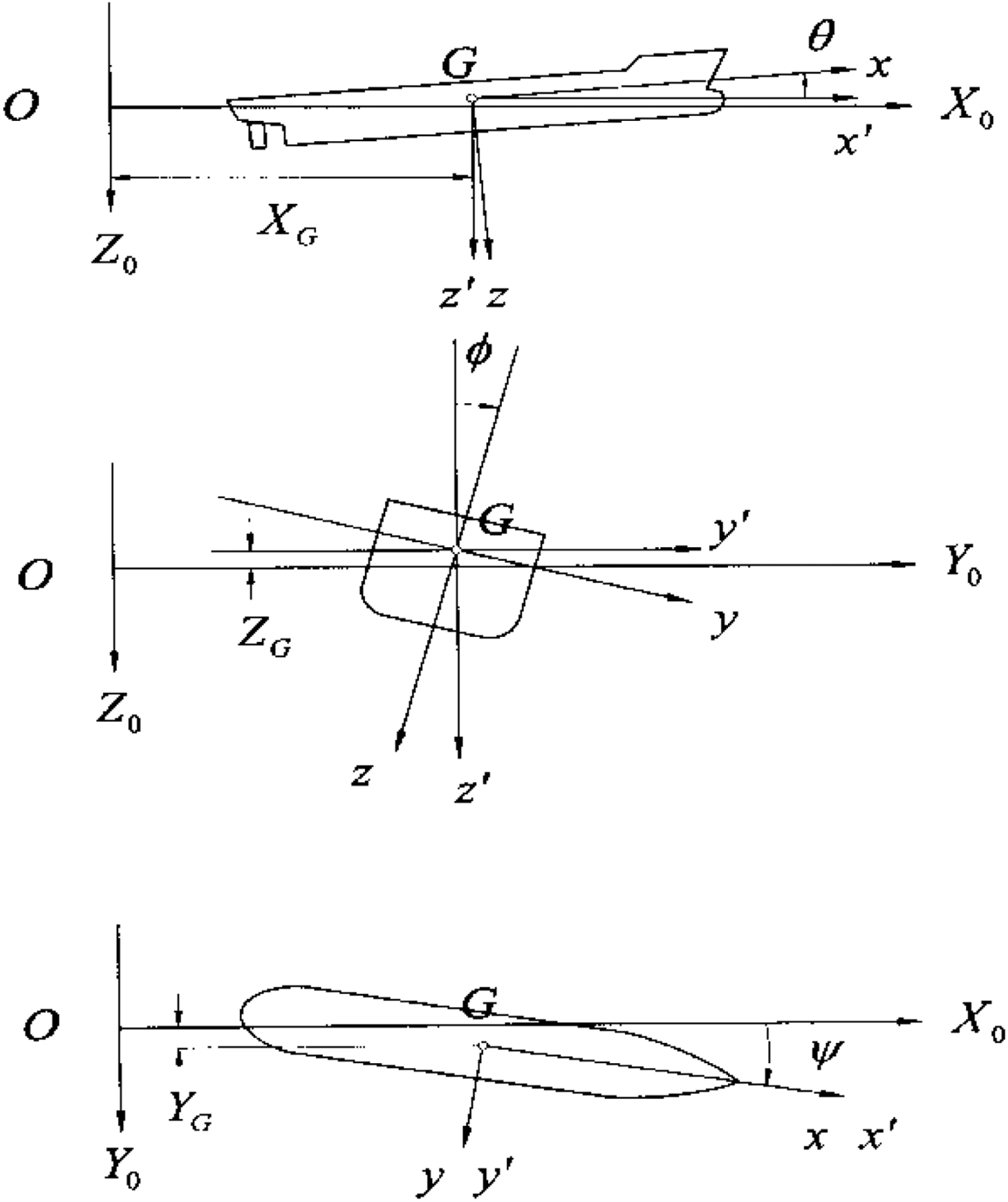
Figure 1. Global coordinate system (UMS).

The horizontal body coordinate system is used to describe the equations of motion. Equations of motion with six degrees of freedom for the ship in waves can be written as below (Fang and Luo, Reference Fang and Luo2006),

(1)$$m(\dot{u}-v\dot{\psi})=(m_y-X_{v\dot{\psi}})v\dot{\psi}-m_x\dot{u}-m_zw\dot{\theta}+X_{FK}+X_{RF}+T(1-t_p)-R$$

(2)$$\eqalign{m(\dot{v}-u\dot{\psi})=&-m_xu\dot{\psi}-m_y\dot{v}-Y_vv+Y_{\dot{\psi}}\dot{\psi} +Y_{v \vert v \vert }v \vert v \vert +Y_{v \vert \dot{\psi} \vert }v \vert \dot{\psi} \vert \cr & +Y_{\dot{\psi} \vert \dot{\psi} \vert }\dot{\psi} \vert \dot{\psi} \vert +Y_{FK}+Y_{DF}+Y_{RF}}$$

(3)$$m\dot{w}=-m_z\dot{w}-Z_ww+Z_{\ddot{\theta}}\ddot{\theta}-Z_{\dot{\theta}}\dot{\theta}-Z_\theta\theta +Z_{FK}+Z_{DF}+mg$$

(4)$$I_{xx}\ddot{\phi}-I_{xx}\dot{\theta}\dot{\psi}=J_{xx}\dot{\theta}\dot{\psi}-J_{xx}\ddot{\phi} -K_{\dot{\phi}}\dot{\phi}+(Y_vv-Y_{\dot{\psi}}\dot{\psi})Z_H+K_{FK}+K_{DF}+K_{RF}$$

(5)$$I_{yy}\ddot{\theta}+I_{xx}\dot{\psi}\dot{\phi}=-J_{xx}\dot{\phi}\dot{\psi}-J_{yy}\ddot{\theta}-M_{\dot{\theta}}\dot{\theta} +M_\theta\theta-M_{\dot{w}}\dot{w}-M_ww+M_{FK}+M_{DF}$$

(6)$$\eqalign{ I_{zz}\ddot{\psi}-I_{xx}\dot{\theta}\dot{\phi}=&J_{xx}\dot{\theta}\dot{\phi}-J_{zz}\ddot{\psi}-N_{\dot{v}}\dot{v} -N_vv-N_{\dot{\psi}}\dot{\psi}+N_{\dot{\psi} \vert \dot{\psi} \vert }\dot{\psi} \vert \dot{\psi} \vert \cr & +N_{vv\dot{\psi}}v^2\dot{\psi} +N_{v\dot{\psi}\dot{\psi}}v\dot{\psi}^2+N_\phi\phi +N_{v \vert \phi \vert }v \vert \phi \vert +N_{\dot{\psi} \vert \dot{\phi} \vert }\dot{\psi} \vert \phi \vert \cr & +(-Y_vv+Y_{\dot{\psi}}\dot{\psi} +Y_{v \vert v \vert }v \vert v \vert +Y_{v \vert \dot{\psi} \vert }v \vert \dot{\psi} \vert +Y_{\dot{\psi} \vert \dot{\psi} \vert }\dot{\psi} \vert \dot{\psi} \vert)x_H \cr & +N_{FK}+N_{DF}+N_{RF}}$$

(7)$$2\pi I_{pp}\dot{n}=Q_E-Q_P$$

where m and I are ship mass and mass moment of inertia, respectively. X, Y and Z are external forces with respect to surge, sway and heave and K, M and N are external moments, with respect to roll, pitch and yaw. u, v and w are surge, sway and heave velocities, respectively, and ϕ, θ and ψ are roll, pitch and yaw displacements, respectively. In Equations (1)–(7), the related sectional added mass and damping coefficients can be calculated using the Frank close-fit method. The $\lpar m_{y}-X_{v\dot{\psi}}\rpar $ term can be written as C _mm _y, and C _m is approximately 0.5–0.75. The m _x, m _y and m _z terms represent the added masses with respect to x, y and z axes respectively, and J _xx, J _yy and J _zz represent the added moments of inertia with respect to x, y and z axes, respectively. The manoeuvring derivatives of the sway and yaw motions can be estimated using empirical formulae (Inoue et al., Reference Inoue, Hirano and Kijima1981). The terms I _PP, Q _E, Q _P represent the moment of inertia of the propeller-shafting system, the propeller torque, and the main engine torque, respectively. The subscripts FK, DF and RF represent the Froude-Krylov forces, the diffraction forces and the rudder forces, respectively.

To build the simplified model, we first assume that the ship's motion simulation excludes environmental factors such as the wind, current and waves, by using the UMS. Additionally, we incorporate the second-order equation of motion proposed by Nomoto (Reference Nomoto1964) into the numerical model to investigate the turning characteristics of the container ship. The second-order model is given as follows:

(8)$$T_1T_2\ddot{r}+(T_1+T_2)\dot{r}+r=K\delta +KT_3\dot{\delta}$$

where K, T ₁, T ₂, and T ₃ are the manoeuvring indices, r is the turning rate, and δ is the rudder angle. The solution of turning rate r can be solved as

(9)$$r(t)=K\delta\left\{1-\displaystyle{{T_1-T_3}\over{T_1-T_2}}\exp\left(-\displaystyle{{t}\over{T_1}}\right) -\displaystyle{{T_3-T_2}\over{T_1-T_2}}\exp\left(-\displaystyle{{t}\over{T_2}}\right)\right\}$$

3. COMPUTATIONAL RESULTS AND DISCUSSIONS

To validate the manoeuvring mathematical model, we selected the sea trial measurements of the C-3 container ship. During the sea trial, the C-3 container ship was in the ballast condition, and the wind was in the range of two to four on the Beaufort scale. The sea trial of ship C-3 was carried out in the Taiwan Strait. The International Maritime Organization (IMO) has established standards of ships' manoeuvring characteristics (IMO, 2002) to ensure minimum safety standards. The turning ability is the measure of the ability to turn the ship using 35° rudder angles. The criteria of advance at a 90° change of heading should not exceed 4.5 ship lengths, and the criteria of Tactical Diameter (TD) defined by the transfer at a 180° change of heading should not exceed 5.0 ship lengths. Table 1 shows the principal particulars of the container ship.

Table 1. Principal particulars of the C-3 container ship.

Figures 2 and 3 show the trajectory for 35° rudder starboard and port turns of the container ship in deep water conditions. Figure 2 shows the starboard turning trajectory of the C-3 container ship travelling at 26.7 knots. It is observed that the difference between simulation results and the sea trial measurements is small for the tactical diameter of the ship; the sea trial measurement is 1,451 m, whereas the numerical simulation is 1,435.1 m when the change of ship heading is 180°. Small discrepancies are also found in advance simulation, that is, the sea trial measurement is 1,125 m, whereas the numerical simulation is 1,189.6 m when the change of ship heading is 90°.

Figure 2. Trajectory of 35° starboard turn for C-3 container ship.

Figure 3. Trajectory of 35° port turn for C-3 container ship.

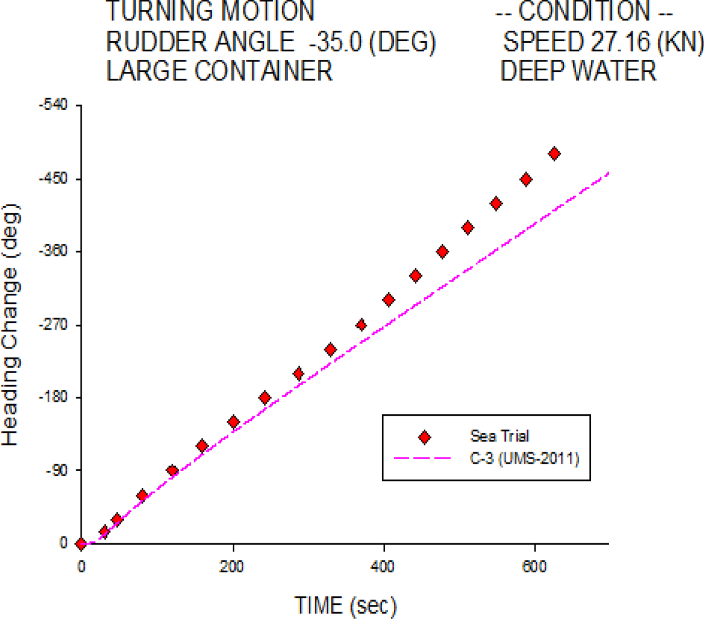
Figure 3 shows the port turning trajectory of the C-3 container ship travelling at 27.16 knots. The simulated tactical diameter is 1,428.9 m, and the measured tactical diameter is 1,336 m when the change of ship heading is 180°. Larger discrepancies are observed when the heading change is over 270°; however, the discrepancies in simulated advance are small; the sea trial measurement of advance is 1,204 m, and the numerical simulation is 1,185 m when the change of ship heading is 90°. All results satisfy the IMO standards, and are shown in Table 2.

Table 2. Comparison of turning circle test of the C-3 container ship.

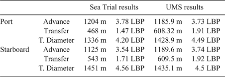
Table 2 shows the validation results of the turning circle test. Good correlations are found in the initial turning stage when the change of the ship's heading is within 90°. However, when the simulation approaches the steady turning situation, the nonlinear behaviours of the ship turning are observed from the sea trial measurements. This may come from the hydro-meteorological factors. As this paper focuses on emergency collision avoidance, the results of the initial turning stage have been adopted.

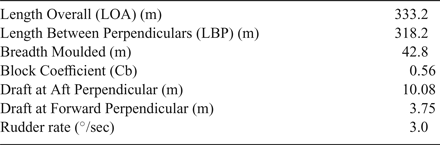
Figure 4 shows the starboard turning rate histories of the C-3 container ship travelling at 26.7 knots. The numerical simulation is validated by the sea trial measurements. The simulated steady turning rate is 0.637°/sec, whereas the measured one is 0.690°/sec. Excellent agreement is found in the initial turning stage, whereas small discrepancies exist in the final stage, which may be due to the drift effects of currents during the sea trial.

Figure 4. Turning rate of 35° starboard turn for the C-3 container ship.

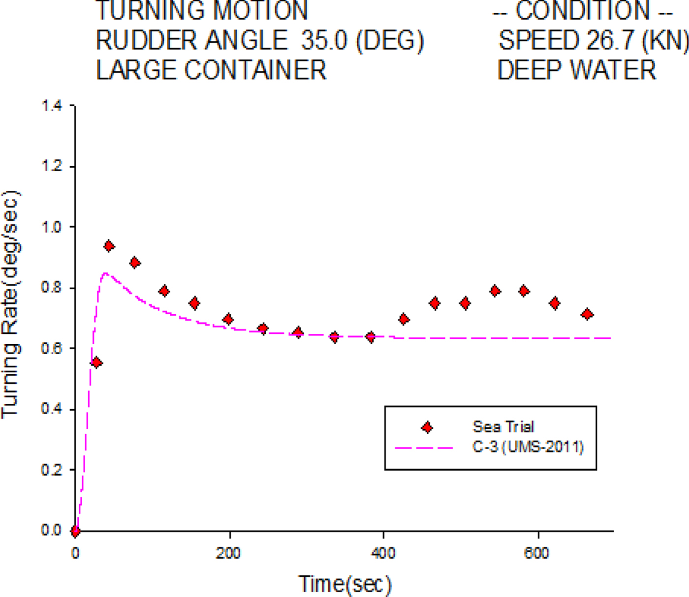
Figure 5 shows the port turning rate histories of the C-3 container ship at 27.16 knots. Similar to the starboard case in Figure 4, the numerical simulation is well validated overall, except in the final stage. The simulated steady turning rate is 0.635°/sec, and the measured one is 0.746°/sec. Small discrepancies in the final stage might also come from current drift effects during the sea trial.

Figure 5. Turning rate of 35° port turn for the C-3 container ship.

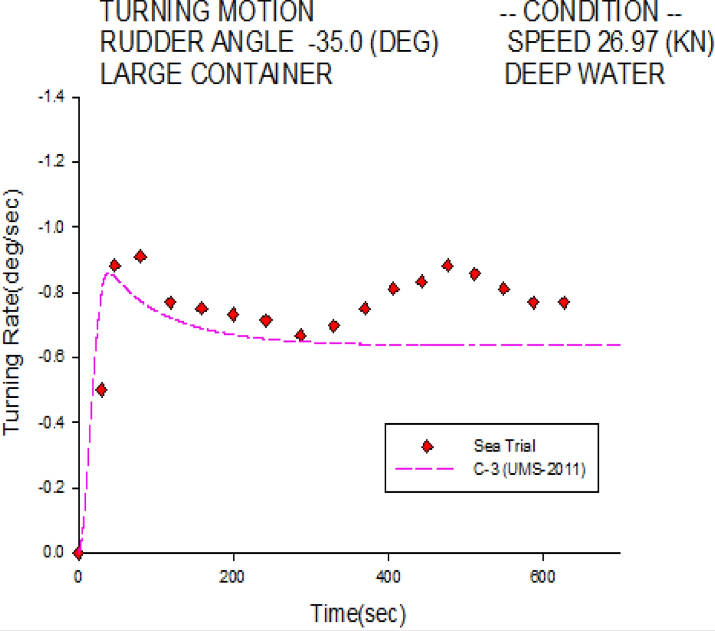
Figure 6 investigates the starboard heading change histories of the C-3 container ship at 26.7 knots. The simulation results agree overall with the sea trial measurements, especially in the initial turning stage. Figure 7 shows the port heading change histories; the numerical simulation is also validated well overall, except in the final stage.

Figure 6. Heading change of 35° starboard turn for the C-3 container ship.

Figure 7. Heading change of 35° port turn for the C-3 container ship.

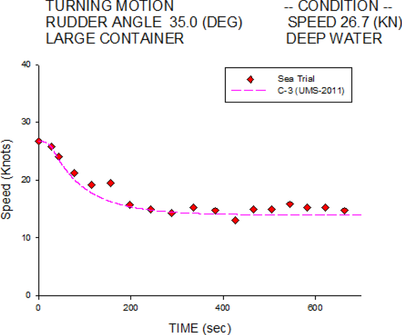
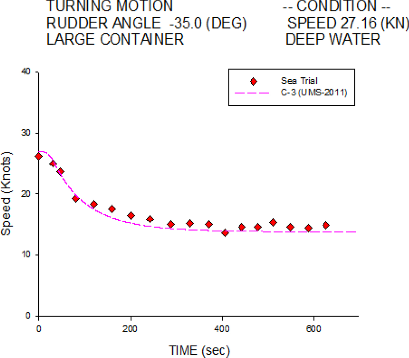
Figures 8 and 9 show the starboard and port turning speed histories, respectively. Agreements are found between the numerical simulations and the sea trial measurements.

Figure 8. Speed histories of 35° starboard turn for the C-3 container ship at 26.7 knots.

Figure 9. Speed histories of 35° port turn for the C-3 container ship at 27.16 knots.

The manoeuvring derivatives of the sway and yaw motions are obtained from the validation of turning sea trial at design speeds. These manoeuvring derivatives have been assumed to keep constant in the present MMG model for different speeds. This may cause some discrepancies at slow speeds due to the limitation of sea trial data, but the performances of resistance, propeller torque and rudder force of the C-3 container ship are modelled from the experimental data in the simulator for all speed ranges. This is a practical solution for a ship simulator, together with having an experienced sea captain to work with us to adjust the ship performance at slow speeds, due to the limitation of sea trial data.

Based on the above validation of the turning characteristics of the C-3 container ship, a series of related numerical results are obtained using the UMS program with respect to varied rudder angles and forward speeds. These findings are summarised in the following part of the paper.

Figures 10 to 15 show the simulation results of the starboard and port turning characteristics of the C-3 container ship with respect to three forward speeds (14.55, 20.12 and 26.7 knots) and seven rudder angles ranging from 5° to 35°. The results in these six figures show that all tactical diameters, advance responses, and transfer responses decrease with the rudder angle, and the effect of speed is not significant.

Figure 10. Tactical diameter of starboard turn for the C-3 container ship.

Figure 11. Tactical diameter of port turn for the C-3 container ship.

Figure 12. Advance of starboard turn for the C-3 container ship.

Figure 13. Advance of port turn for the C-3 container ship.

Figure 14. Transfer of starboard turn for the C-3 container ship.

Figure 15. Transfer of port turn for the C-3 container ship.

The manoeuvring indices, K, T1, T2 and T3, can be obtained from the numerical simulations of turning rate histories using Equation (9) and the regression technique. Figure 16 shows an example of turning rate histories at a 20° starboard turn obtained from the simulations of the C-3 container ship with varied speeds (14.55, 20.12 and 26.7 knots).

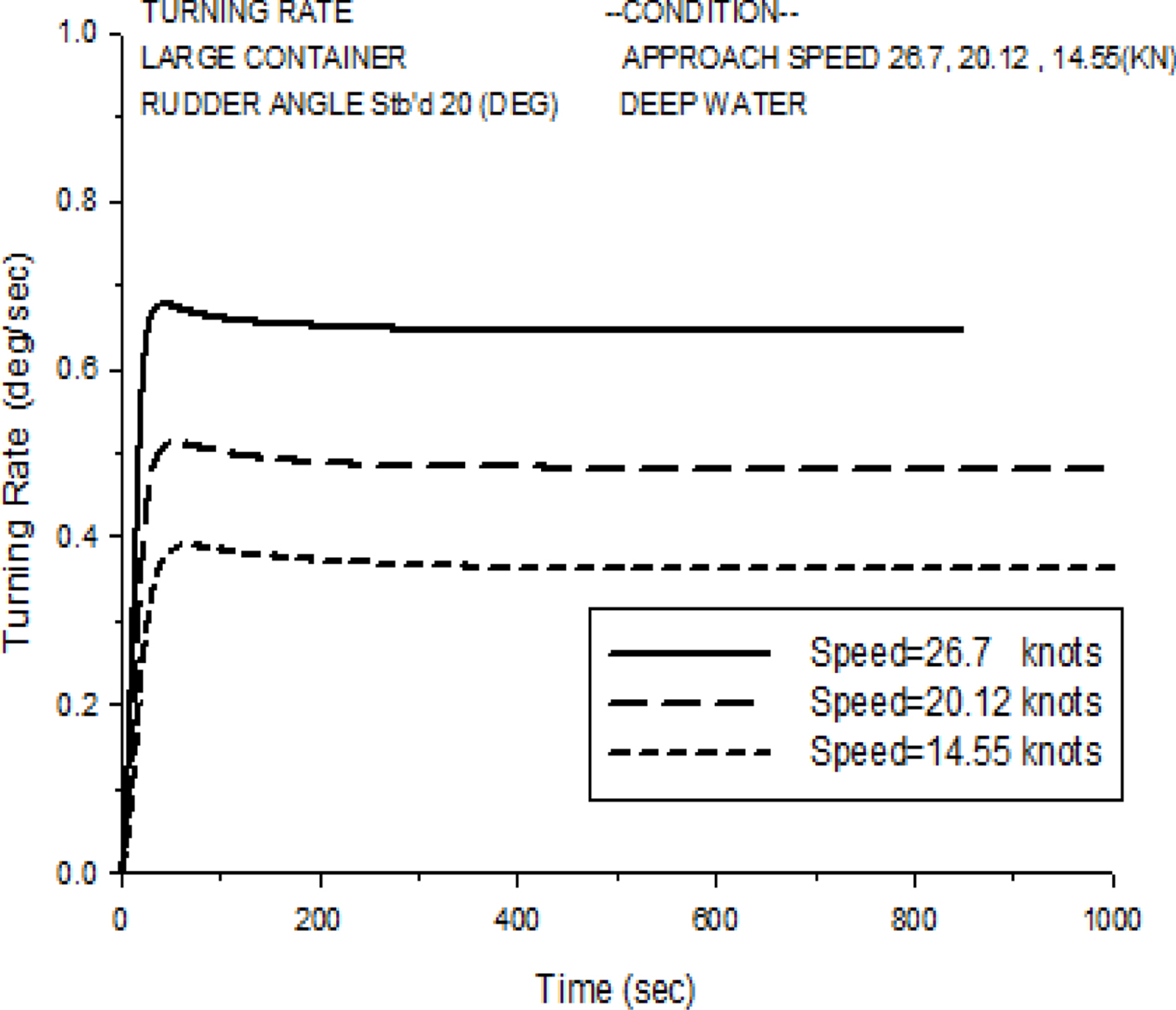
Figure 16. Turning rate histories of a 20° starboard turn for the C-3 container ship with varied speeds.

The K value can be obtained from the numerical simulations using the two-dimensional regression technique with respect to three forward speeds (14.55, 20.12 and 26.7 knots) and rudder angles (5° to 35°), as below:

(10)$$K=0.002679+0.003435U-0.000793\ln\delta\cdot U$$

where U is the ship speed and δ is the rudder angle. Figure 17 shows the two-dimensional regression model of the K value based on the numerical simulation results of the UMS program.

Figure 17. Regression model of K value for the C-3 container ship.

The manoeuvring indices, T1, T2 and T3, are solved by MATLAB software using the Newton-Raphson method to solve the nonlinear equation and the data obtained from numerical simulation. Then, we use the two-dimensional regression technique with three different forward speeds (14.55, 20.12 and 26.7 knots) and rudder angles (5° to 35°) to obtain the following equations:

(11)$$T_1=60.0147-1.6614\delta-2.5329U+0.0325\delta U+0.0237\delta^2+0.035U^2$$

(12)$$T_2=-170.860236+5652.188596/U+58.890545\ln(\delta)-1401.216267\cdot \ln(\delta)/U$$

(13)$$T_3=-88.563572+3262.016155/U+4.783375\delta-76.527108\delta/U$$

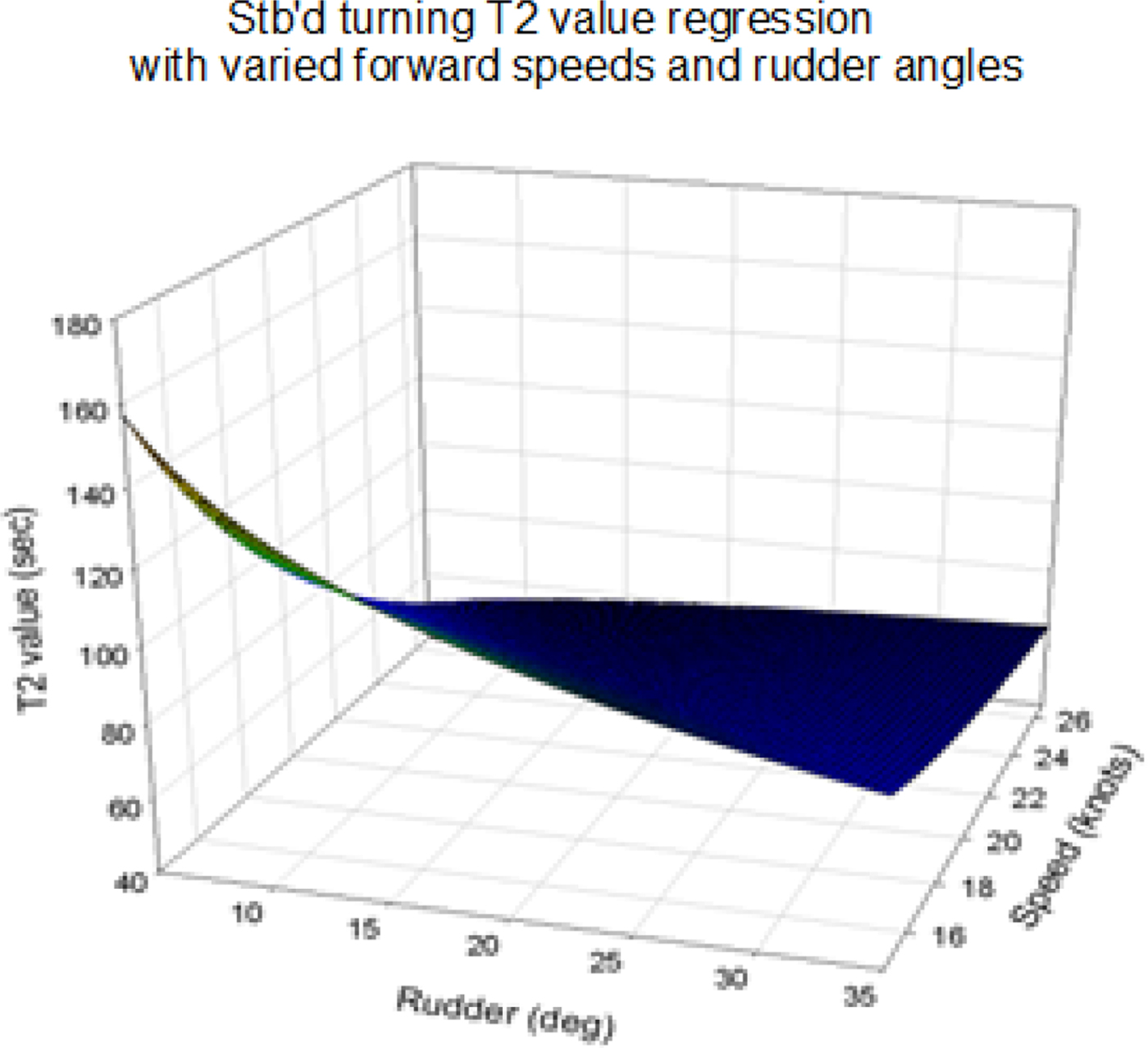
where U is the ship speed and δ is the rudder angle. Figures 18 to 20 show the two-dimensional regression model of T1, T2 and T3 values based on the numerical simulation results of the UMS program.

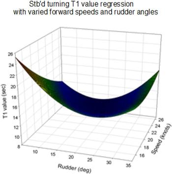
Figure 18. Regression model of T1 value for the C-3 container ship.

Figure 19. Regression model of T2 value for the C-3 container ship.

Figure 20. Regression model of T3 value for the C-3 container ship.

The turning rate histories of the large container ship can then be obtained based on the Nomoto second-order model with the calculated values of K, T1, T2 and T3 from Equations (10) to (13).

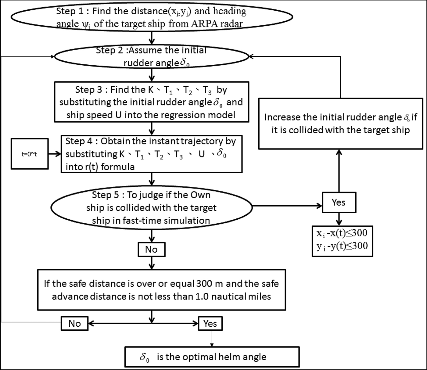
Based on the study of Fang and Tsai (Reference Fang and Tsai2014), the ship's collision avoidance steering system can effectively predict the ship's manoeuvring at low speed with large rudder angles. When the ship enters a harbour at low speed, the captain usually orders large rudder angles to manoeuvre the ship according to his experience. In this study, we assume that the effective collision avoidance rudder angle is at least 10° for the simulations in the traffic area. The safe domain of the ship is assumed to be 300 metres along the side of the moving ships. This figure is to some extent arbitrary, and is set for heavy traffic areas and would need adjusting for more open sea. The proposed ship domain is an ellipsoidal shape at the centre of the ship (Fujii and Tanaka, Reference Fujii and Tanaka1971). The acting time of the rudder will be at least 1.0 nautical mile in advance of the own ship to the moving ships in the traffic area. If the distance to the target ships at the action time is less than 1.0 nautical mile, the initial rudder angle is 10°. However, if the final prediction of the rudder angle is over 35°, when the advance distance is 1.0 nautical mile, the ships will collide. To enhance the ship collision avoidance system with respect to different traffic factors, simple and complex collision avoidance cases are selected to validate the presented simplified ship collision model, which is helpful for navigators in selecting a safe and energy-efficient navigation route. Figure 21 is the flow chart of the optimal helm angle for ship collision avoidance prediction based on the present model. Step 1 of this simulation model involves positioning the target ships, determined by the distance and heading angle, using radar or the Automatic Identification System (AIS) on board in each time step.

Figure 21. The optimal helm angle for ship collision avoidance.

After determining the information for the target ships, step 2 assumes an initial rudder angle, δ₀, for the first simulation, and step 3 involves calculating the manoeuvring indices, K, T1, T2 and T3, from Equations (10)–(13). The calculations are based on the ship's speed, U, and initial rudder angle, δ₀, which are established in advance using the Newton-Raphson method with respect to the three different forward speeds and seven different rudder angles from the UMS simulations. Step 4 is conducted to obtain the instantaneous trajectories of the own ship by substituting K, T1, T2, T3, U and δ into Equation (9). Based on the predicted trajectories of the own ship and numerical recursion techniques, step 5 of the simulation model involves judging whether the own ship will collide with the target ships, using a fast-time simulation to examine the helm angle of the own ship. If the simulated own ship collided with the target ships, this simulation model will increase the initial rudder angle, δ₀, by 1° intervals. If the own ship is too far away from the target ships, the model will decrease the initial rudder angle, δ₀, at 1° intervals. This is a fast-time simulation process for collision avoidance. Until the helm order can reach the optimal conditions for a safe and energy-efficient navigation route, that is, achieving a transverse safe domain (in a heavy traffic area this is set to be 300 metres, which is about seven times the ship's breadth and is proposed by the senior captain), or the safe advance distance is 1.0 nautical mile, the rudder will start to operate based on the helm order. After the own ship safely passes the position at a safe distance, the rudder angle should follow the helm order to turn back to its initial course using an autopilot algorithm.

This study simulated three different collision conditions (head-on, overtaking, and crossing situations) for two non-uniformly moving ships using the ship collision avoidance system. In all simulation cases, the collision avoidance decision making should follow the Convention on the International Regulations for Preventing Collisions at Sea (COLREGS, 1972).

3.1. Head-on condition (simple)

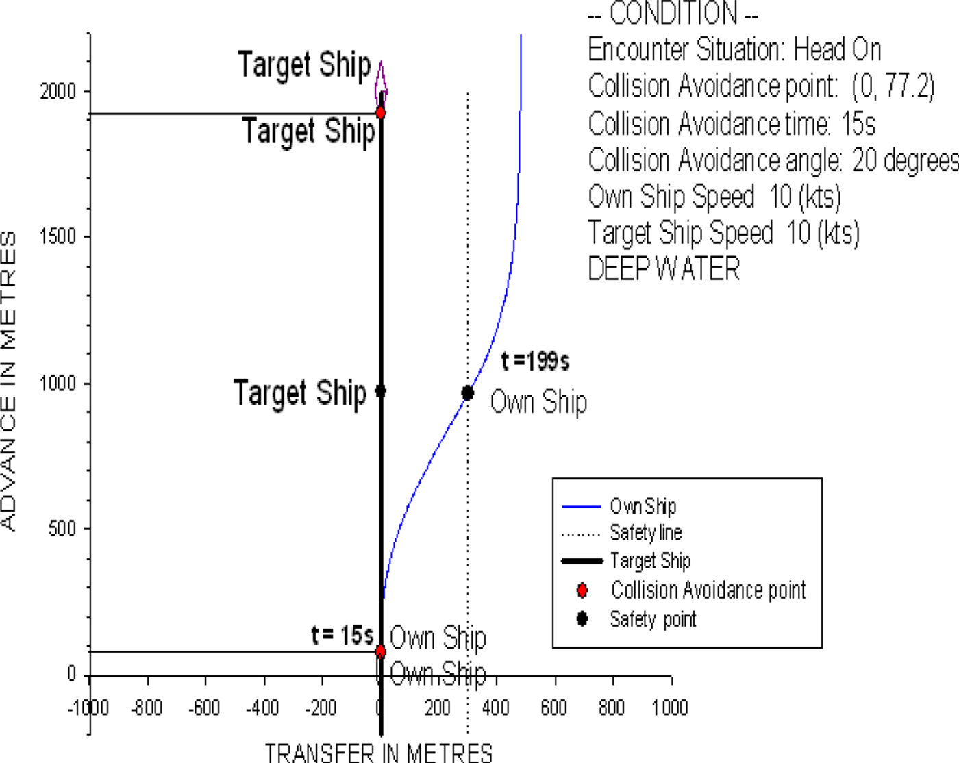
Figure 22 shows a ship trajectory for the head-on condition of two non-uniformly moving ships. The own ship, the C-3 container ship, is travelling at a speed of 10 knots with a heading of 0° (northward). The target ship is 2,000 metres in front of the own ship and sails on a course of 180° (southward) at 10 knots. In the head-on condition, the own ship should alter her course to starboard so that each shall pass on the port side of the other (COLREGS, 1972. Rule 14). Based on the prediction of the present ship collision avoidance model, the time for the collision avoidance manoeuvre is at t = 15 s, and the optimal rudder angle is 20°, obtained from the collision avoidance model. With this helm order, the own ship starts to operate the rudder to alter course until she keeps 300 metres away from the target ship, and it then turns back to the initial northward course.

Figure 22. The ship trajectory for the head-on condition of two non-uniformly moving ships.

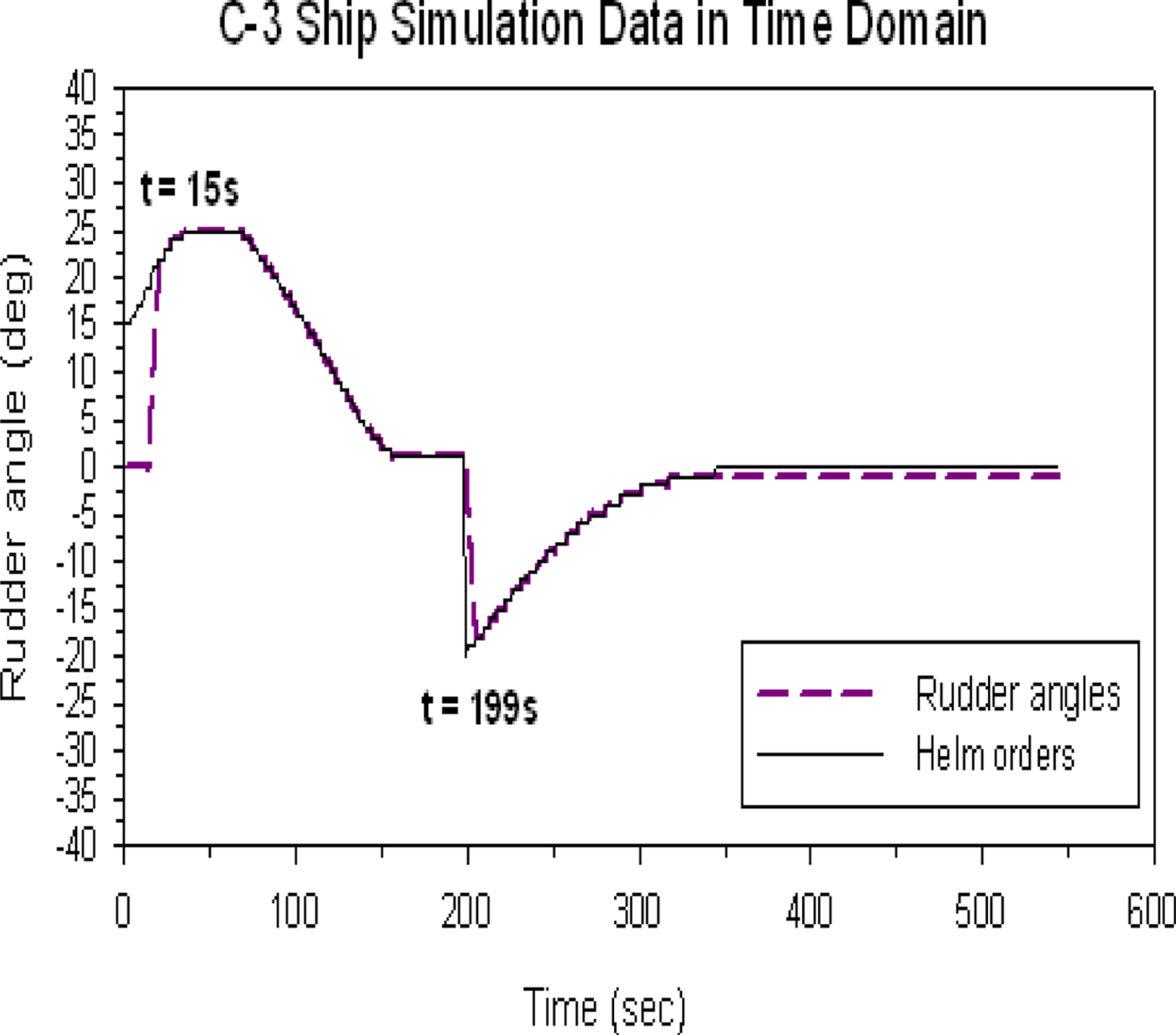
Figure 23 shows the time history of the predicted helm order and rudder operation. Although the predictions of the helm order are calculated from the beginning of the simulation, the rudder is kept still until the predicted helm order reaches the optimal rudder angle of 20°, that is, at the collision avoidance time t = 15 s. Then, the system model continues to calculate and modify the helm order at every instant for the ship's trajectory followed by the rudder operation until the own ship reaches the safe position, that is, a distance of 300 metres from the port side of the target ship at around t = 199 s. Then, we use an autopilot-type algorithm to turn the own ship back to its initial course, for example, if the optimal initial rudder angle is starboard at 20°, we initially use port 20° to adjust the course and turn back to the initial course. Based on this operation, the own ship can safely pass the target ship and finally turn safely back to its initial course.

Figure 23. The time history of the predicted helm order and rudder operation of the head-on condition.

3.2. Overtaking condition (simple)

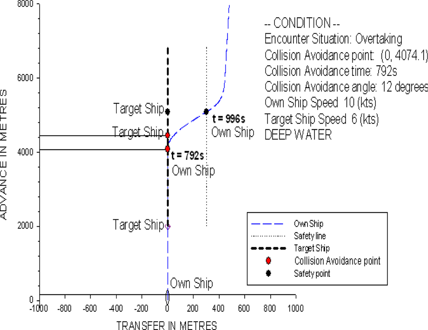
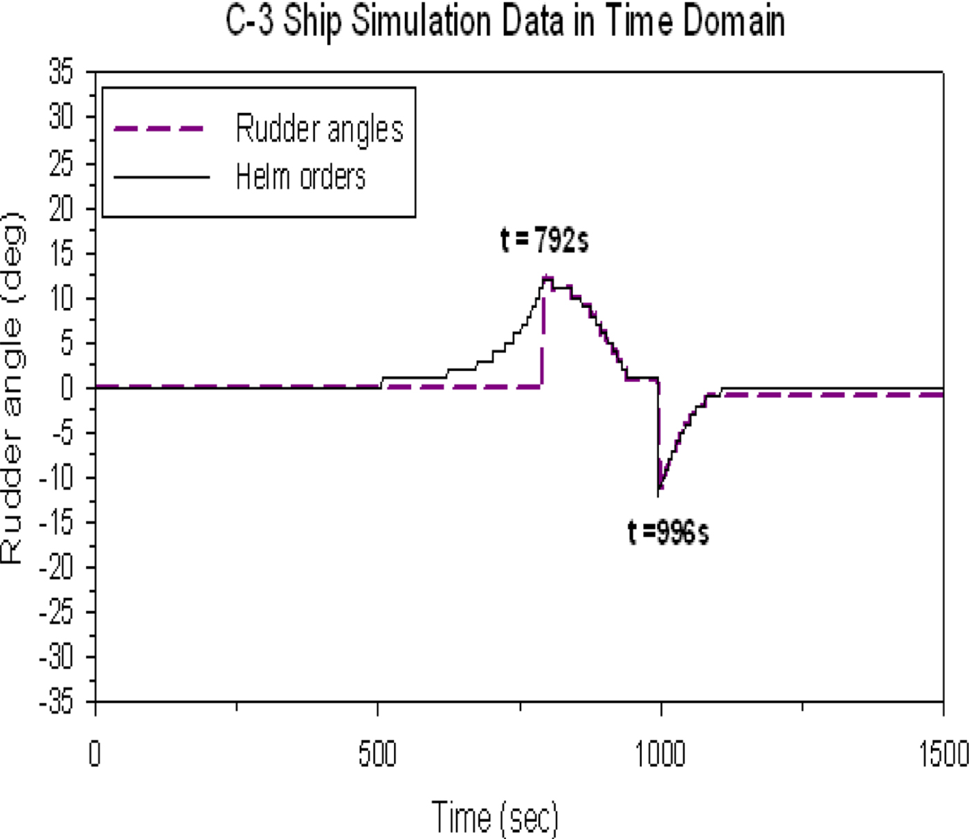
According to Rules 9 and 34 of the COLREGS (1972), the own ship may overtake the target ship on either side and can indicate her intention by giving clear signals with a whistle. In this study, the starboard side overtaking scenario is selected for discussion. There is no limitation for our model to carry out a port side overtaking scenario. Figure 24 shows that the own ship is travelling at 10 knots with a heading of 0°, and the target ship is 2,000 metres in front of the own ship and keeps its course at a speed of 6 knots. The time for collision avoidance is at t = 792 s, and the optimal rudder angle is 12° predicted by the ship collision avoidance model. When the own ship reaches the safe location, that is, 300 metres away from the target ship to the right, it turns back to its original course.

Figure 24. The ship trajectory for the overtaking condition of two non-uniformly moving ships.

Figure 25 also shows the time history of the predicted helm order and rudder operation for reference. However, similar discussions can be referred to those in Figure 23. The time of rudder operation of the own ship to turn back to her initial course is at t = 996 s.

Figure 25. The time history of the predicted helm order and rudder operation of the overtaking condition.

3.3. Crossing condition (simple)

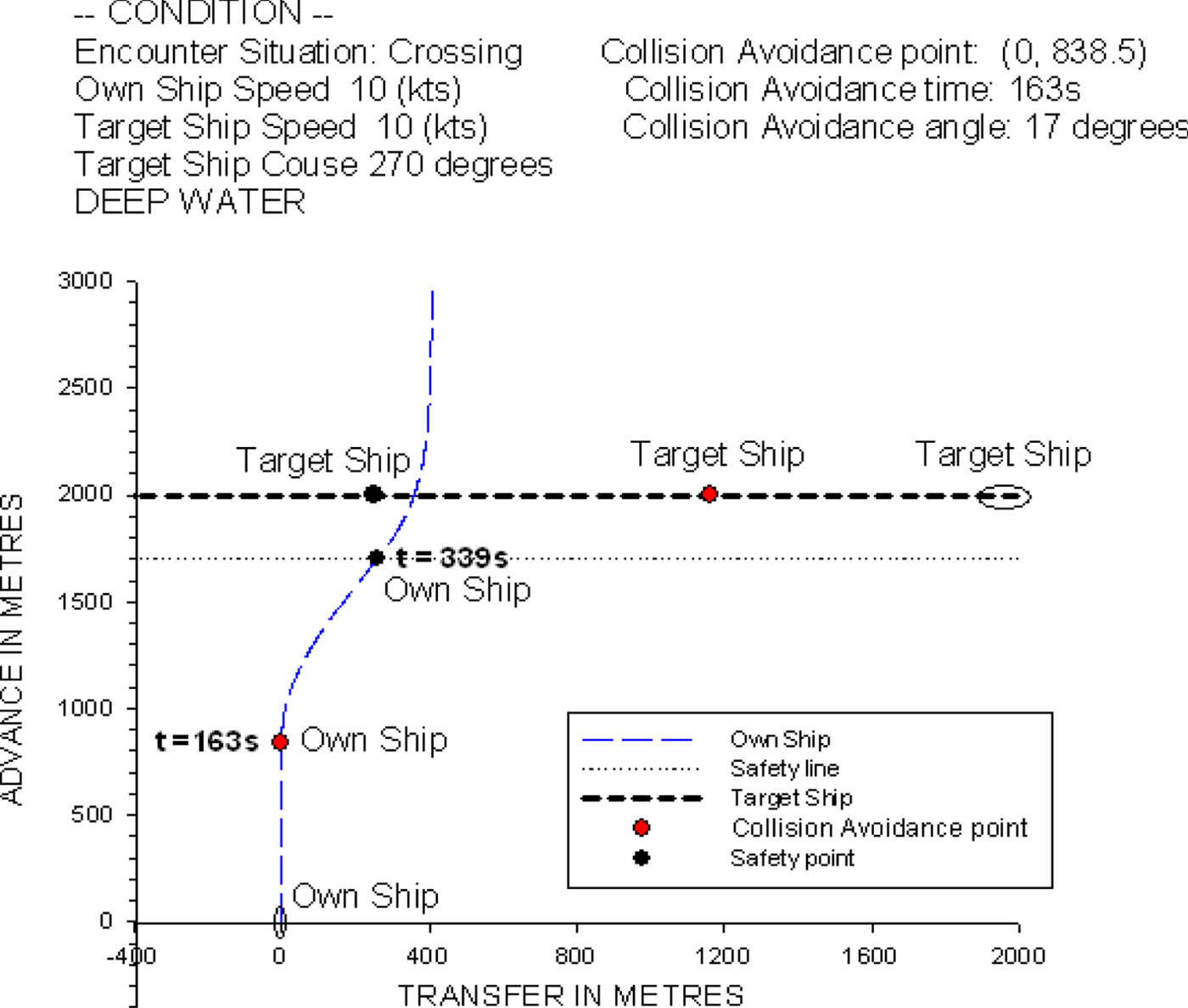
Figure 26 shows that the own ship is travelling at 10 knots with a heading of 0°. The target ship's speed is 10 knots and the heading is 270°, i.e., approaching from the starboard side of the own ship at a distance of 2,000 metres. According to the COLREGS (1972), the own ship is the give-way vessel and the target ship is the stand-on vessel. The own ship should take action to avoid a collision, and the target ship should stay on a steady course. In this case, the predicted collision avoidance time and optimal rudder angle are at t = 163 s and 17°, respectively, calculated by the present ship collision avoidance model.

Figure 26. The ship trajectory for the crossing condition of two non-uniformly moving ships.

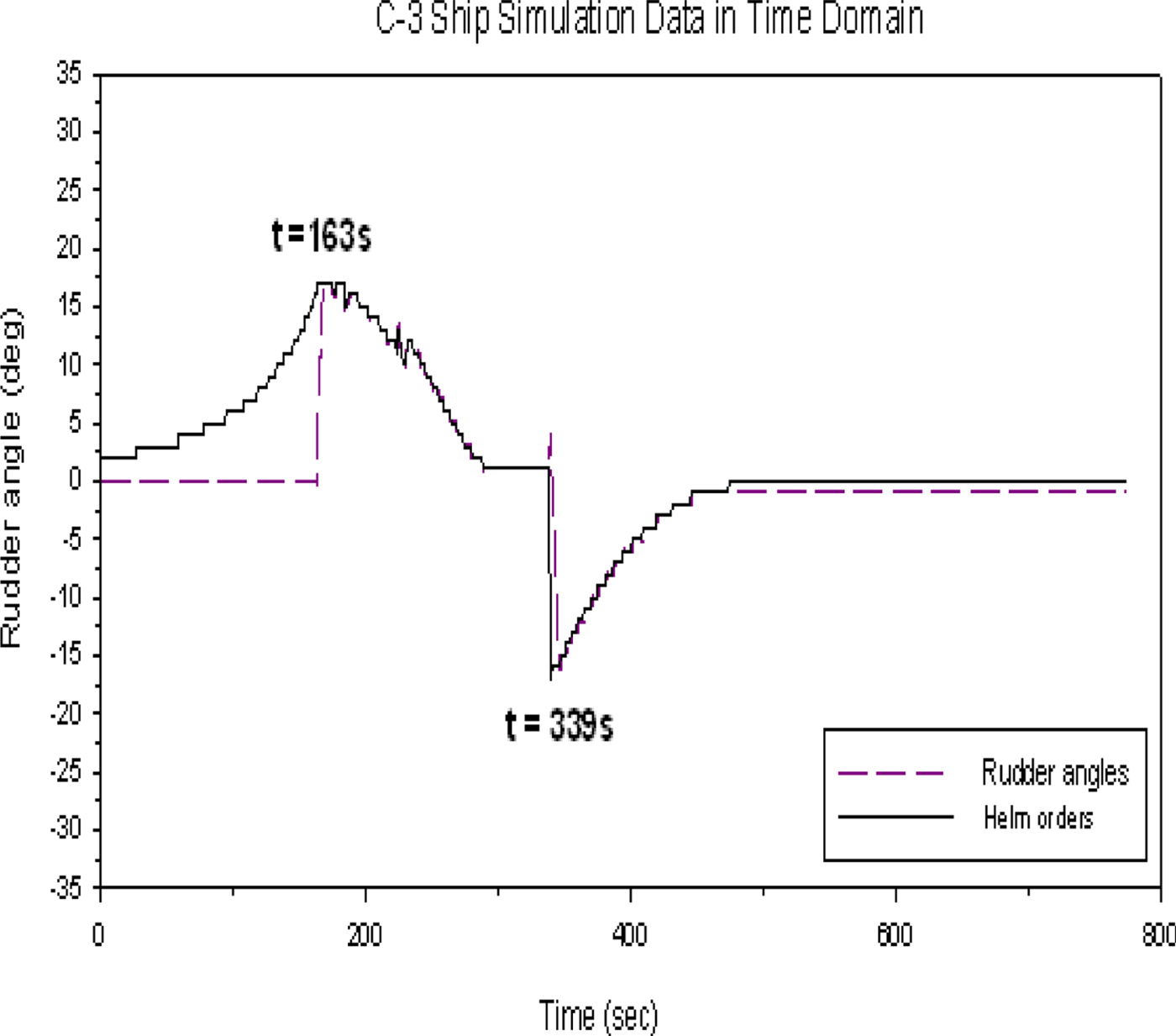
Figure 27, which is the time histories of the predicted helm order and rudder operation, shows that the own ship keeps its course until the helm order reaches the optimal rudder angle of 17°. After the optimal helm order of 17° is achieved, the own ship operates the rudder and follows a similar procedure as was stated in Figure 23 to avoid the target ship and turn back to her initial course. The time of rudder operation for the own ship to turn back to her initial course is at t = 339 s.

Figure 27. The time history of the predicted helm order and rudder operation of the crossing condition.

The three simulation results indicate that the ship collision avoidance model can provide a suitable helm order for the own ship to pass the target ship safely.

Next, two complex collision conditions with three non-uniformly moving ships, including head-on and crossing conditions, are selected for simulation verification using the ship collision avoidance system model.

3.4. Head-on condition (complex)

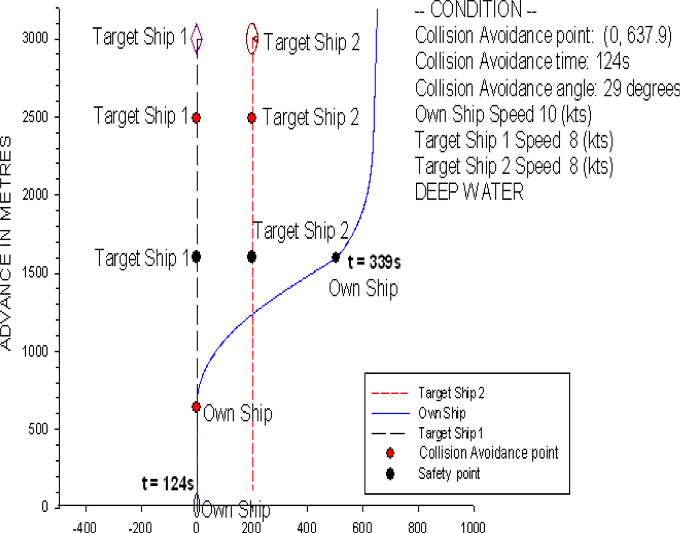
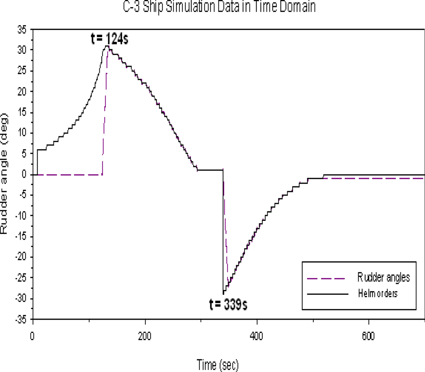
Figure 28 shows that the own ship is travelling at 10 knots with a heading of 0°. Both target ships 1 and 2 are 3,000 metres in front of the own ship, and the clearance between the two ships is 300 metres. The travelling speed and heading for both target ships are set at 8 knots and 180°s, respectively. In this case, we also assume the safe distance is at least 300 metres from every target ship; therefore, the own ship can only sail away to the port side of target ship 2 to avoid colliding with both target ships. The time for collision avoidance action is at t = 124 s and the optimal rudder angle is 29°, which are predicted by the model. When the own ship achieves a distance of 300 metres, target ship 2 starts to turn back to her initial course at t = 339 s. Figure 29 shows the time history of the predicted helm order and rudder operation. In this case, similar discussions can be made as for the case in Figure 23 after the collision avoidance action. The results in Figure 29 show that the own ship can keep the rudder angle constant, that is, at the optimal rudder angle of 29° until she reaches the safe distance of 300 metres. Then, the own ship needs to use the port rudder angle of 29° to turn back to her initial course at t = 339 s.

Figure 28. The ship trajectory for the head-on condition of three non-uniformly moving ships.

Figure 29. The time history of the predicted helm order and rudder operation of the head-on condition.

3.5. Crossing condition (complex)

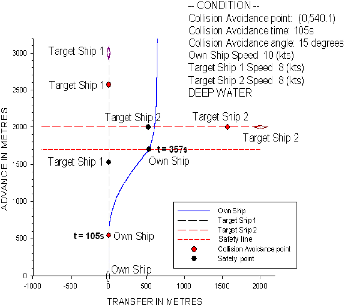
The complex crossing condition in Figure 30 shows that the own ship is travelling at 10 knots with a heading of 0°. Target ship 1 is 3,000 metres in front of the own ship with a heading of 180° and a speed of 8 knots. Target ship 2 approaches from the starboard side of the own ship at a distance of 2,000 metres, a heading of 270° and a speed of 8 knots. First, the ship collision avoidance system judges which target ship is more dangerous to the own ship. In this case, if the advance distance of target ship 1 is more than 1.0 nautical miles to the own ship, target ship 2 is more dangerous to the own ship. According to the COLREGS (1972), the own ship is the give-way vessel and target ship 2 is the stand-on vessel. Therefore, the own ship should take action to avoid a collision, and the target ship should maintain its course. From the calculations by the ship collision avoidance model, the time for the collision avoidance action is at t = 105 s, and the optimal rudder angle is 15°. Figure 30 shows the related trajectory of the simulation for this complex crossing condition.

Figure 30. The ship trajectory for the crossing condition of three non-uniformly moving ships.

Figure 31 shows the time history of the predicted helm order and rudder operation. Similar procedures can be followed to those shown in Figure 23. The time of rudder operation for the own ship to turn back to her initial course is at t = 357 s.

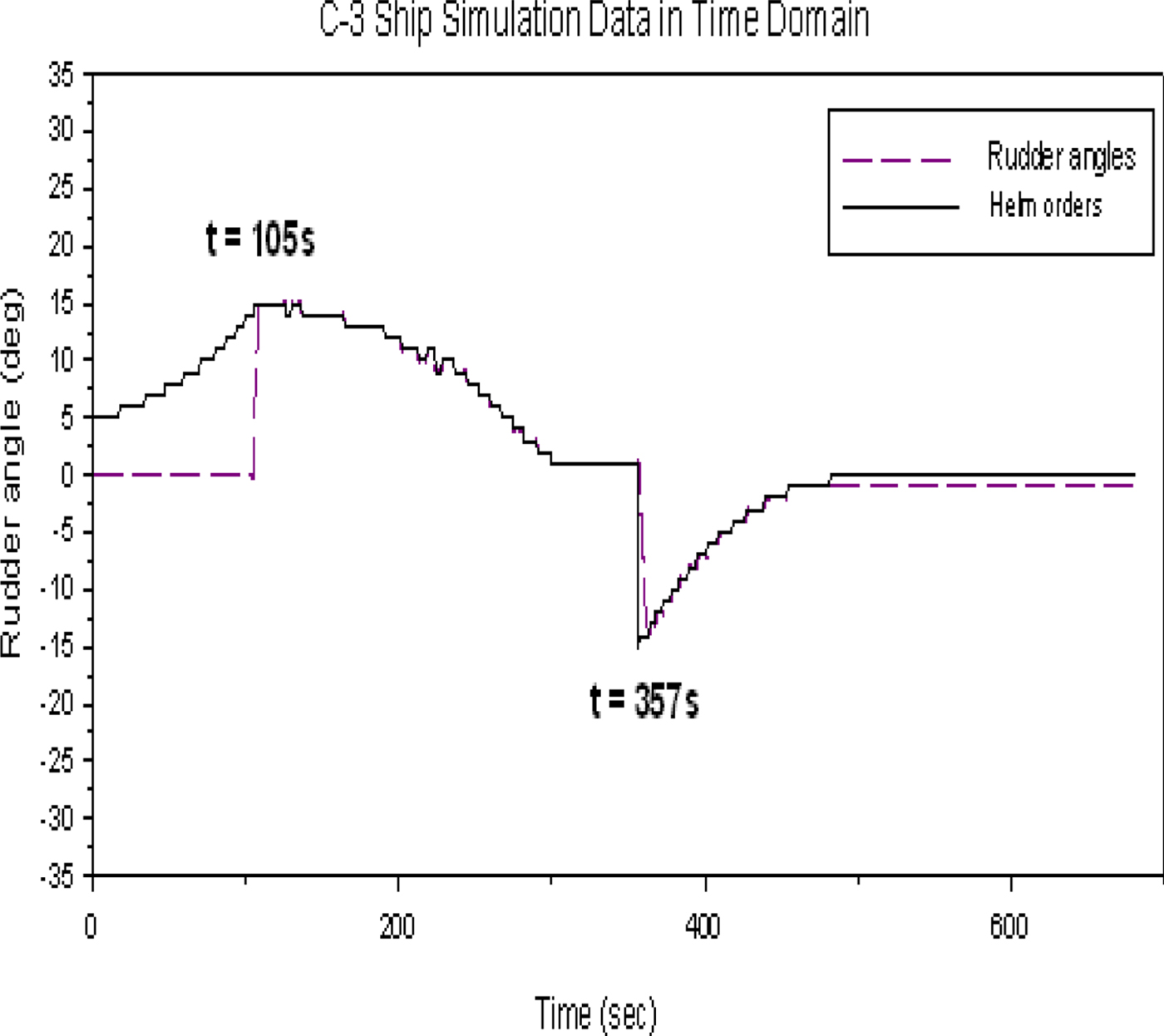
Figure 31. The time history of the predicted helm order and rudder operation of the crossing condition.

Based on the two complex simulation results, we can verify that the ship collision avoidance model can be easily applied to obtain the optimal rudder angle with respect to complex conditions for the own ship to pass target ships safely.

The verification studies show that the ship collision avoidance model, based on the database of manoeuvring indices, is effective at obtaining the optimal rudder angle for ship collision avoidance with respect to different cases in a heavy traffic area.