I. INTRODUCTION
One of the reasonable configurations for laboratory powder diffraction measurement systems is currently the combination of (i) a Cu-target sealed tube in the orientation of line-focus geometry, (ii) a couple of Soller slits on the incident and diffracted beam sides, (iii) Ni-foil Kβ filter, (iv) flat powder specimen, and (v) Si strip one-dimensional (1D) detector. Since the transmittance of the Ni foil of 0.02 mm in thickness is about 0.44 for CuKα and 0.007 for CuKβ X-rays, insertion of a Ni foil effectively reduces the diffraction peak caused by CuKβ emission from the Cu-target X-ray tube. The use of a Johan-type or Johanson-type monochromator, or a graded multilayer mirror on the incident beam side, or a curved graphite analyzer on the diffracted beam side may be another possible choice to remove CuKβ peaks. However, the use of a monochromator, multilayer mirror or analyzer generally causes theoretical complexity for modeling the spectroscopic characteristics of the source X-ray, because mutual correlation between the direction and wavelength of the X-ray beam should be introduced by such a diffractive optical element (Toraya and Hibino, Reference Toraya and Hibino2000). Furthermore, only slight misalignment of a diffractive optical element may cause severe distortion of the observed diffraction peak profile (Ida et al., Reference Ida, Hibino and Toraya2001).
We have previously demonstrated that CuKα 2 sub-peaks can be removed by a deconvolution–convolution method, from the diffraction intensity data collected with a conventional laboratory powder diffractometer, where the diffracted beam intensities measured on the diffraction angle, 2θ-scale of abscissa, are mapped onto the scale-transformed abscissa, x ≡ ln sinθ. This article is intended to demonstrate that the method is also effective to remove both CuKβ sub-peaks and NiK-edge step structures from the powder diffraction data collected with a laboratory powder diffraction measurement system with a Ni-foil filter.
II. THEORETICAL
A deconvolution–convolution method to remove the effects of axial-divergence, flat-specimen and sample-transparency aberrations in Bragg–Brentano geometry has been described in our previous report (Ida and Toraya, Reference Ida and Toraya2002). The details of slight improvement about the treatment of axial-divergence aberration, which has already been applied in this study, will be discussed elsewhere (Ida et al., Reference Ida, Ono, Hattan, Yoshida, Takatsu and Nomura2018). This article is focused on the methodology to remove CuKα 2 and Kβ peaks and NiK-edge structures from experimental data.
A. Scale transform of abscissa
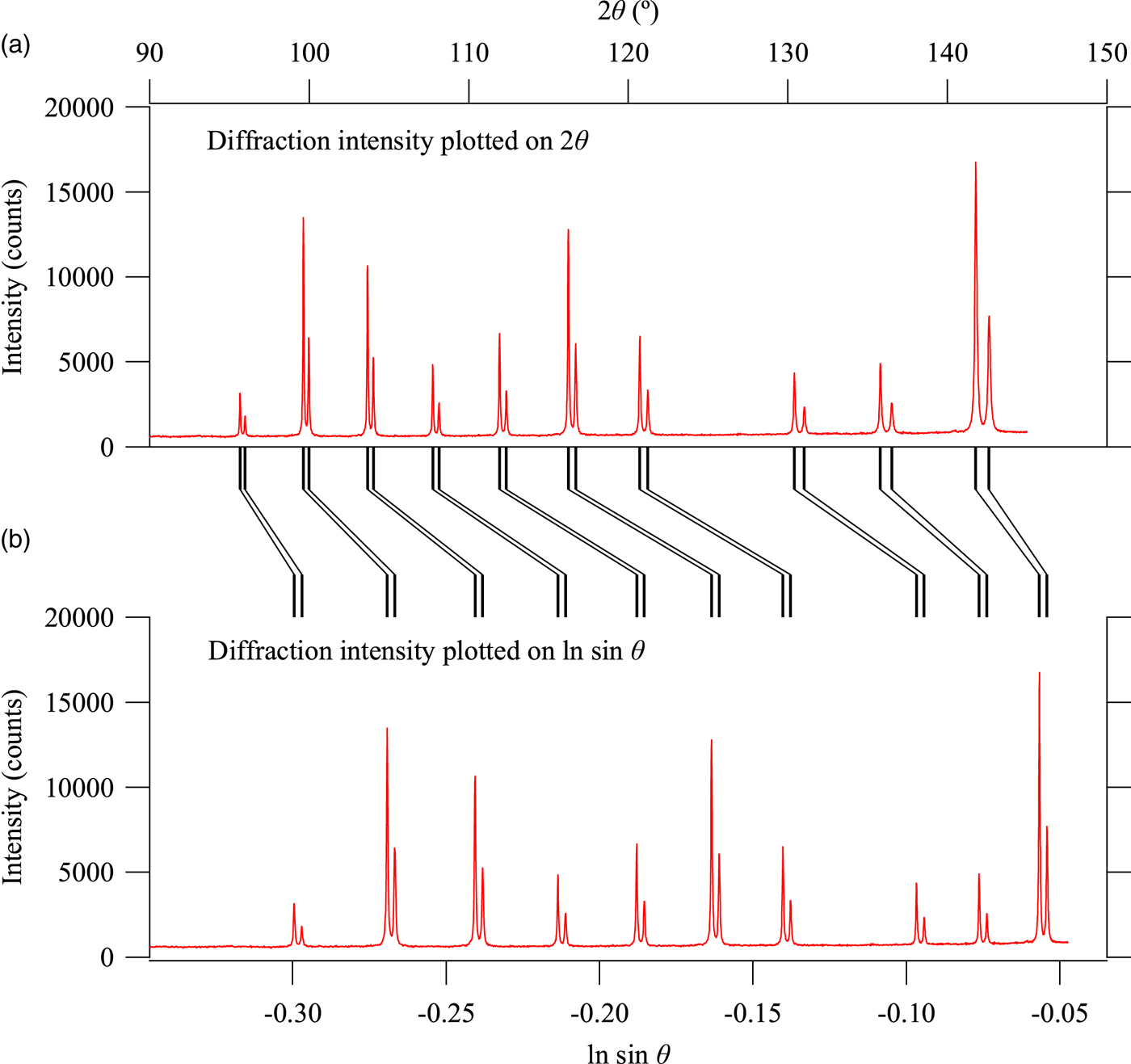
When the diffraction intensity profile is plotted on the abscissa scale of x = ln sinθ instead of the diffraction angle 2θ, whole powder diffraction data can be expressed as the convolution with the common spectroscopic profile function of source X-ray (Ida and Toraya, Reference Ida and Toraya2002). Figure 1 illustrates the core idea about the scale transform. Observed powder diffraction profile of LaB6 is plotted on the diffraction angle 2θ in Figures 1(a) and 1(b) plots exactly the same intensity data on the natural logarithm of sinθ. Each of reflection peaks is composed of Kα 1 and Kα 2 peaks, and the separation of Kα 1 and Kα 2 peaks varies on the horizontal scale of 2θ, while it is constant on the horizontal scale of x = ln sinθ. In other words, the diffraction intensity profile is expressed by the convolution with the common instrumental function about spectroscopic profile of the source X-ray on the scale of x = ln sinθ, but it is not a convolution on the scale of 2θ.

Figure 1. Diffraction intensity data of LaB6 plotted on (a) 2θ and (b) ln sin θ.
When the observed data are given by a set of diffraction angles and intensities (2θ, I), the abscissa and ordinate values are changed to (x, y) by the following equations,
 $$x = \ln \sin \theta, $$
 $$y = 2IC\,(2\theta )\tan \theta, $$
where C (2θ) is the geometric correction factor given by
 $$C\,(2\theta ) = \displaystyle{{2\sin \theta \sin 2\theta} \over {1 + {\cos} ^22\theta}}, $$
for a Bragg–Brentano powder diffractometer without a diffractive optical element.
After the scale-transformed data (x, y) are changed to (x′, y′) by the deconvolution–convolution process, the intensity will be treated by
 $${I}^{\prime} = \displaystyle{{{y}^{\prime}} \over {2C(2\theta )\tan \theta}}, $$
to obtain the modified intensity data on the original 2θ scale, (2θ, I′).
B. Emission of Cu-target X-ray
Assuming the peak energy and wavelength of the CuKα 1 emission to be E α1 = 8.04783 keV (Deutsch et al., Reference Deutsch, Förster, Hölzer, Härtwig, Hämäläinen, Kao, Huotari and Diamant2004) and λα1 = 1.5405929Å, we here apply the transformation given by
 $$x = \ln \displaystyle{{E_{\alpha 1}} \over E} = \ln \displaystyle{\lambda \over {\lambda _{\alpha 1}}},$$
for arbitrary photon energy E and wavelength λ. A model for spectroscopic profile of the source X-ray, f X(x), is given by
 $$f_{\rm X}(x) = f_\alpha (x) + S_{\beta /\alpha} f_\beta \,(x) + S_{\rm B}(x),$$
where f α(x) and f β(x) are the normalized CuKα and Kβ emission peak profile functions, S β/α the CuKβ/CuKα intensity ratio, and S B(x) the contribution of the white X-ray caused by bremsstrahlung.
The CuKα emission peak profile is expressed by
 $$f_\alpha (x) = \mathop \sum \limits_{i = 1}^2 \mathop \sum \limits_{\,j = 1}^2 \displaystyle{{2I_{\alpha ij}} \over {\pi \Delta x_{\alpha ij}}}\left[ {1 + 4{\left( {\displaystyle{{x - x_{\alpha ij}} \over {\Delta x_{\alpha ij}}}} \right)}^2} \right]^{ - 1},$$
 $$x_{\alpha ij} = \ln \displaystyle{{E_{\alpha 1}} \over {E_{\alpha ij}}}\; \approx \displaystyle{{E_{\alpha 1} - E_{\alpha ij}} \over {E_{\alpha 1}}},$$
 $$\Delta x_{\alpha ij} \approx \displaystyle{{W_{\alpha ij}} \over {E_{\alpha ij}}},$$
where the values of intensity I αij, location E αij, and peak width W αij of the component Lorentzian functions given in a literature (Deutsch et al., Reference Deutsch, Förster, Hölzer, Härtwig, Hämäläinen, Kao, Huotari and Diamant2004) are listed in Table I.
Table I. Peak energy E, full width at half maximum W and integrated intensity I for doublet and quartet models for CuKα emission and a quintet model for CuKβ emission (Deutsch et al., Reference Deutsch, Förster, Hölzer, Härtwig, Hämäläinen, Kao, Huotari and Diamant2004).
The CuKβ emission peak profile is similarly expressed by
 $$f_\beta (x) = \mathop \sum \limits_{i = 1}^5 \displaystyle{{2I_{\beta i}} \over {\pi \Delta x_{\beta i}}}\left[ {1 + 4{\left( {\displaystyle{{x - x_{\beta ij}} \over {\Delta x_{\alpha ij}}}} \right)}^2} \right]^{ - 1},$$
 $$x_{\beta i} = \ln \displaystyle{{E_{\alpha 1}} \over {E_{\beta i}}},$$
 $$\Delta x_{\beta i} \approx \displaystyle{{W_{\beta i}} \over {E_{\beta i}}},$$
where the values of component intensity I βi, location E βi, and peak width W βi are also listed in Table I.
The contribution of white X-ray, S B(x) in Eq. (6), should be dependent on (i) the acceleration voltage and target material of the X-ray tube, (ii) absorption and scattering of beryllium window of the sealed tube and atmosphere through the X-ray beam path from the X-ray source to the detector, (iii) energy-dependent sensitivity of the detector, and also (iv) the settings of the pulse-height discriminator or analyzer.
Trincavelli et al. (Reference Trincavelli, Castellano and Riveros1998) have proposed a formula for the spectroscopic distribution of the bremsstrahlung given by
 $$\eqalign{\displaystyle{{\Delta I} \over {\Delta E}} & = \sqrt Z \displaystyle{{E_0 - E} \over E} \cr & \left[ { - 54.86 - 1.072E + 0.2835E_0 + 30.4\ln Z + \displaystyle{{875} \over {Z^2\; E_0^{0.08} \;}}} \right],} $$
where Z is the atomic number of the target material, E 0 the upper limit of the photon energy in the unit of keV, and E the photon energy of the X-ray. The intensity distribution on the scale of x = ln (E α1/E) is calculated from ΔI/ΔE by
 $$\displaystyle{{\Delta I} \over {\Delta x}} = \displaystyle{{E\Delta I} \over {\Delta E}}.$$
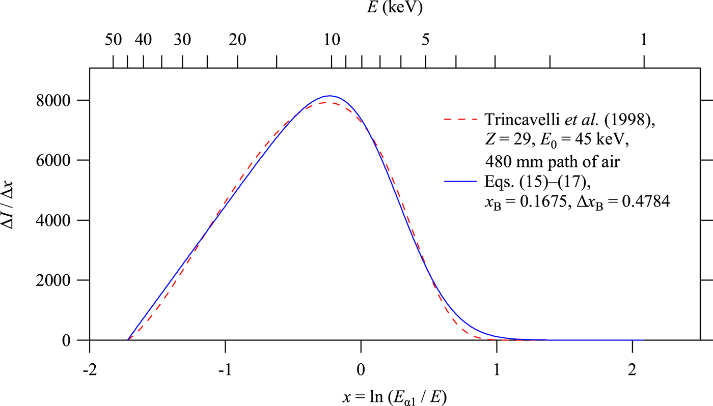
 Figure 2 shows the intensity distribution of the bremsstrahlung calculated by Eq. (13) for Cu target and  $E_0 = 45{\kern 1pt} {\rm keV}$, multiplied by the transmittance of air (4:1 mixture of nitrogen and oxygen) through the path of 480 mm in length, which is calculated by the Cromer–Liberman algorithm (Cromer and Liberman, Reference Cromer and Liberman1981; Cromer, Reference Cromer1983).

Figure 2. White X-ray (bremsstrahlung) spectra calculated by the formula of Trincavelli et al. (Reference Trincavelli, Castellano and Riveros1998) and Eqs (15)–(17).
Here we apply a simplified model for the white X-ray intensities, the normalized formula of which is given by
 $$S_{\rm B}(x) = \left\{ {\matrix{ {\displaystyle{{I_{\rm B}} \over N}\left( {\displaystyle{{x - x_0} \over {\Delta x_{\rm B}}}} \right){\rm erfc}\left( {\displaystyle{{x - x_{\rm B}} \over {\Delta x_{\rm B}}}} \right)} & {\left[ {x_0 \lt x} \right]} \cr 0 & {\left[ {x \le x_0} \right]} \cr}} \right.,$$
 $$N = \displaystyle{{\Delta x_{\rm B}} \over 4}\left[ {(1 + 2t_0^2 )\,{\rm erfc}\,(t_0) - \displaystyle{{2t_0} \over {\sqrt \pi}} \exp \,( - t_0^2 )} \right]\; \;, $$
 $$t_0 = \displaystyle{{x_0 - x_{\rm B}} \over {\Delta x_{\rm B}}},$$
where the integrated intensity of white X-ray I B, and the profile parameters x B and Δx B are treated as adjustable parameters. The lower limit on the scale of x, x 0 = ln (E α1/E 0), which corresponds to the upper limit of the photon energy, may appear to be treated as a fixed parameter determined by the acceleration voltage, but the value can be changed in practical application, because it is likely that the upper limit of the photon energy of the white X-ray to be detected is restricted by the energy-dependent sensitivity of the detector rather than the acceleration voltage. The intensity profile calculated by Eqs (15)–(17) is also shown in Figure 2. Note that almost linear dependence of the peak profile of the function S B (x) on the side of smaller x is dominantly determined by the bremsstrahlung characterized by the parameter x 0, but the intensity for larger x is assumed to be restricted by the extinction by the air, and simulated by adjusting the values of the parameters x B and Δx B.
C. Effect of Ni filter for CuK-emission X-ray source
When a Ni foil is used as a Kβ filter, the virtual spectroscopic profile of the source X-ray, f X:Ni(x), should be given by
 $$f_{{\rm X:Ni}}(x) = T_{{\rm Ni}}(x)f_{\rm X}(x),$$
where T Ni(x) is the transmittance spectrum of the Ni foil, given by
 $$T_{{\rm Ni}}(x) = \exp \left[ { - {(\mu /\rho )}_{{\rm Ni}}(x)\rho _{{\rm Ni}}t_{{\rm Ni}}} \right],$$
where ρ Ni and t Ni are the density and thickness of the Ni foil, respectively, and (μ/ρ)Ni(x) is the mass absorption coefficient spectrum of Ni. The spectrum of (μ/ρ)Ni(x) calculated by the method of Cromer and Liberman (Cromer and Liberman, Reference Cromer and Liberman1981; Cromer, Reference Cromer1983) is further simplified here by the following equation,
 $$\eqalign{(\mu /\rho )_{{\rm Ni}}(x) = \left\{ {\matrix{ {337.58\exp \left[ {2.7130\,(x - x_{{\rm Ni} - K})} \right]} & {\left[ {x \lt x_{{\rm Ni} - K}} \right]} \cr {41.145\exp \left[ {2.8097\,(x - x_{{\rm Ni} - K})} \right]} & {\left[ {x_{{\rm Ni} - K} \le x} \right]} \cr}} \right.,}$$
where x Ni−K = −0.03478 is the location of NiK-absorption edge ( $E_{{\rm Ni} - K} = 8.3327{\kern 1pt} {\rm keV}$) relative to the CuKα 1 peak position.
Figure 3 compares the mass absorption coefficient spectrum calculated by the Cromer–Liberman method and the simplified formula given by Eq. (20). No significant difference between the Cromer–Liberman profile and the profile calculated by Eq. (20) can be detected in the range displayed in Figure 3.
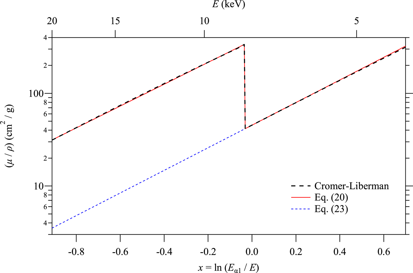
Figure 3. Comparison of the mass absorption coefficient spectra of Ni calculated by the Cromer–Liberman method (thick broken line), a simplified model (thin solid line), and the hypothetical spectrum without K-absorption edge (thin broken line).
D. Hypothetical CuKα 1 singlet spectrum without NiK-absorption edge
Removal of CuKα 2, Kβ sub-peaks and NiK-edge structure can be achieved by deconvolution of the realistic spectroscopic profile modeled in the Sections II.B and II.C, and convolution with a hypothetical spectroscopic profile of a CuKα 1 singlet, the model which will be described in this section.
Hypothetical CuKα 1 singlet spectrum without NiK-absorption edge is expressed by
 $$f_{{\rm X*:Ni*}}(x) = T_{{\rm Ni*}}(x)f_{{\rm X*}}(x),$$
where T Ni*(x) is the transmittance spectrum given by
 $$T_{{\rm Ni*}}(x) = \exp \left[ { - {(\mu /\rho )}_{{\rm Ni*}}(x)\rho _{{\rm Ni}}t_{{\rm Ni}}} \right],$$
where (μ/ρ)Ni*(x) is the hypothetical mass absorption coefficient spectrum of Ni without K-absorption edge, given by
 $$(\mu /\rho )_{{\rm Ni*}}(x) = 41.145\exp \left[ {2.8097(x - x_{{\rm Ni} - K})} \right]\;. $$
As can be seen in the spectrum calculated by Eq. (23) plotted in Figure 3, it is just extrapolation of the spectroscopic profile of Ni in the lower energy (larger x) region.
The function f X*(x) in Eq. (21) is a CuKα 1 singlet spectrum, which we here assume to be
 $$f_{{\rm X*}}(x) = f_{\alpha 1}(x) + f_{\rm B}S_{\rm B}(x),$$
where f α1(x) is given by
 $$f_{\alpha 1}(x) = \displaystyle{{2I_{\alpha 1}} \over {\pi \Delta x_{\alpha 1}}}\left[ {1 + 4{\left( {\displaystyle{{x - x_{\alpha 1}} \over {\Delta x_{\alpha 1}}}} \right)}^2} \right]^{ - 1},$$
which is identical to the Kα 1 component in the Kα 1, Kα 2 doublet model (see Table I).
The parameter f B in Eq. (24) is a factor to adjust the background in the output data. When the white background is fully removed from the input data and not added to the output (f B = 0), it is likely that negative intensities will be created in the background region because of the statistical variation of the observed intensities. Although there will be no reason not to allow negative intensities when the statistical errors are explicitly assumed in subsequent analysis of data, it may be difficult for some users of traditional codes for Rietveld analysis (Rietveld, Reference Rietveld1969) to include explicit error values in their analyses. On the other hand, when the white background is fully added (f B = 1), the background intensities in the output data should naturally be enhanced, because we here assume higher transmittance of Ni without K-absorption as defined by Eq. (23).
E. Deconvolution and convolution treatments
In our previous report (Ida and Toraya, Reference Ida and Toraya2002), we have applied the analytical formula for the Fourier transform of the spectroscopic distribution of the source X-ray. In this study, the Fourier transforms of the model functions are numerically calculated applying the following formulas,
 $$F_{{\rm X}:{\rm Ni}}(k) = \mathop \sum \limits_{\,j = - n/2}^{n/2 - 1} f_{{\rm X}:{\rm Ni}}(\,j{\rm \Delta} x)\exp \left( {\displaystyle{{2\pi ikj} \over n}} \right),$$
 $$F_{{\rm X*}:{\rm Ni*}}(k) = \mathop \sum \limits_{j = - n/2}^{n/2 - 1} f_{{\rm X*}:{\rm Ni*}}(j{\rm \Delta} x)\exp \left( {\displaystyle{{2\pi ikj} \over n}} \right),$$
where Δx is the step interval of the sampling points. The values of Δx and n should be determined not to lose information included in the source data and to keep sufficient width of marginal region to reduce the end effects (Ida and Toraya, Reference Ida and Toraya2002).
The deconvolution–convolution process about intensities  $y_j \to {y}^{\prime}_j$ is expressed by
 $${y}^{\prime}_j = \displaystyle{1 \over n}\mathop \sum \limits_{k = - n/2}^{n/2} \displaystyle{{F_{{\rm X*}:{\rm Ni*}}(k)} \over {F_{{\rm X:Ni}}(k)}}Y_k\exp \left( { - \displaystyle{{2\pi ikj} \over n}} \right),$$
 $$Y_k = \mathop \sum \limits_{j = 0}^{n - 1} y_j\exp \left( {\displaystyle{{2\pi ikj} \over n}} \right),$$
where the values of y j in Eq. (29) are intensity values for the sampling points of x j = x 0 + jΔx, evaluated by cubic-spline interpolation of the source data. Marginal data in the range x 0 + mΔx <x j <x 0 + nΔx for x 0 + mΔx ≈ ln sinθ max were filled with the values given by the following equation,
 $$y_j = \left\{ {\matrix{ {y_m} & {\left[ {m \lt j \lt \displaystyle{{2m + n} \over 3}} \right]} \cr {\displaystyle{{(2n + m - 3j)y_m + (3j - 2m - n)y_0} \over {n - m}}} & {\left[ {\displaystyle{{2m + n} \over 3} \lt j \lt \displaystyle{{m + 2n} \over 3}} \right]} \cr {y_0} & {\left[ {\displaystyle{{m + 2n} \over 3} \lt j \lt n} \right]} \cr}} \right..$$
The fast Fourier transform algorithm can be used for all the calculations of Eqs (26)–(29).
III. EXPERIMENTAL
A. Sample
Standard LaB6 powder (NIST SRM660a) was used as received. The powder was filled into the cavity of a flat glass holder with the capacity of 0.1152 mL and the rectangular cross-section of 20 mm × 15 mm (average depth of 0.384 mm). The filling factor of the powder was estimated at 26.7% by weight measurement, and the penetration depth of the CuKα X-ray into the powder sample was estimated at  $\mu ^{ - 1} = 0.044{\kern 1pt} {\rm mm}$.
B. Data collection
Diffraction data were collected with a powder diffractometer (PANAlytical, X'Pert PRO MPD) with a Cu-target sealed tube, θ–θ type goniometer (PANAlytical, PW3050/60) equipped with a 1D Si strip detector (PANAlytical X'Celerator). The X-ray source and the detector are symmetrically located at the distance of 240 mm from the rotation axis of the goniometer. The X-ray tube was operated at the voltage of 45 kV and the current of 40 mA. Fixed-angle divergence slit of 0.5° and a couple of Soller slits with the open angle of 0.04 rad were used. Ni foil of 0.02 mm in thickness was used as a Kβ filter. The 1D powder diffraction intensity data of 8079 sampling points were created by an automatic measurement/data processing program (PANAlytical, Data Collector) from the integration of five iterations of continuous scan for the diffraction angles ranging from 10° to 145° with the nominal step interval of 0.0167° and nominal measurement time of 10.16 s per step. The total measurement time for data collection was about 1 h.
IV. RESULTS AND DISCUSSION
Figure 4 shows the background intensity profile of LaB6 (NIST SRM660a) and the deconvolved–convolved intensity profile calculated on some variation of parameters, (i) the upper limit of X-ray photon energy, E 0 and (ii) the output white X-ray level, f B, while other adjustable parameters for the model of white X-ray are fixed as follows, (iii) CuKβ/α intensity ratio S β/α = 0.2, (iv) white X-ray intensity relative to CuKα 1, I B = 0.4, (v) relative location of the decay of the white X-ray on the lower energy side, x B = 0.17, and (vi) the decay-width parameter, Δx B = 0.48.
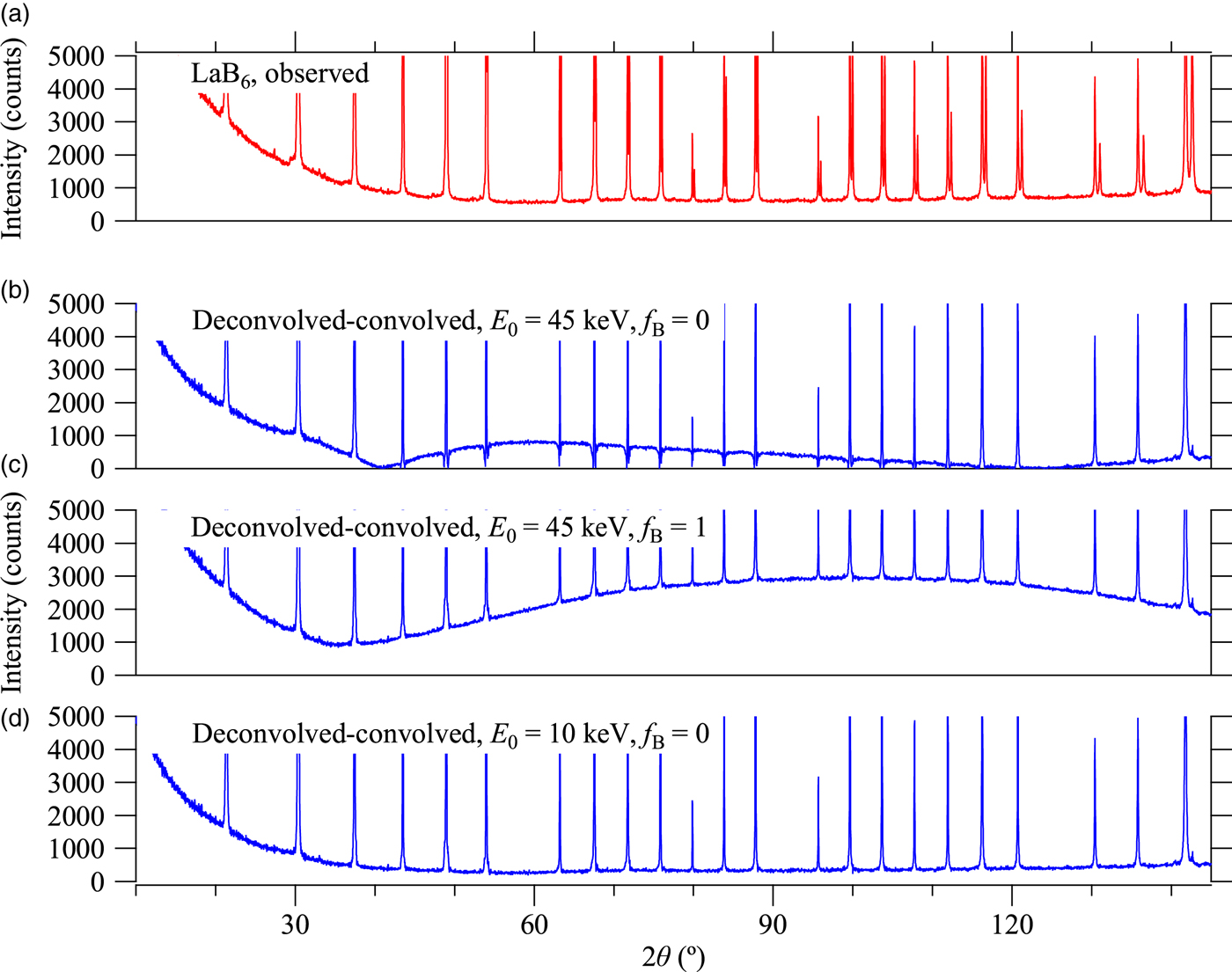
Figure 4. (a) Overall background profile of observed diffraction data of LaB6 powder measured with a Cu-target X-ray tube and Ni-foil Kβ filter, and the deconvolved–convolved data calculated with the parameters (b) E 0 = 45 keV and f B = 0, (c) E 0 = 45 keV and f B = 1, (d) E 0 = 10 keV and f B = 0.
It should be noted that the CuKα 2 peaks have effectively been removed in the deconvolved–convolved data, just by applying the parameters proposed by Deutsch et al. (Reference Deutsch, Förster, Hölzer, Härtwig, Hämäläinen, Kao, Huotari and Diamant2004) without any modification or adjustment. As can be seen in Figures 4(b) and 4(c), severe deformation of the background profile has appeared in the deconvolved–convolved data, when the upper limit of the photon energy E 0 is set to the acceleration voltage of 45 keV. Hereafter, E 0 = 10 keV and f B = 0 are assumed, because both CuKβ peaks and NiK-edge structures are effectively removed without deformation of the background profile in the deconvolved–convolved data calculated for those values, as shown in Figure 4(d).
Figure 5 compares the background intensity profile of the (a) observed and (b) deconvolved–convolved data in the lower angle region including 100, 110, and 111-reflection peaks of LaB6. The calculated locations of Kβ peaks and NiK-absorption edges for 100, 110, and 111-reflection peaks are marked by vertical arrows in Figure 5. Since the reduction of Kβ peaks is simply achieved by adjusting the value of CuKβ/α intensity ratio S β/α without changing other parameters, there is almost no ambiguity about the assumed value of S β/α = 0.2.
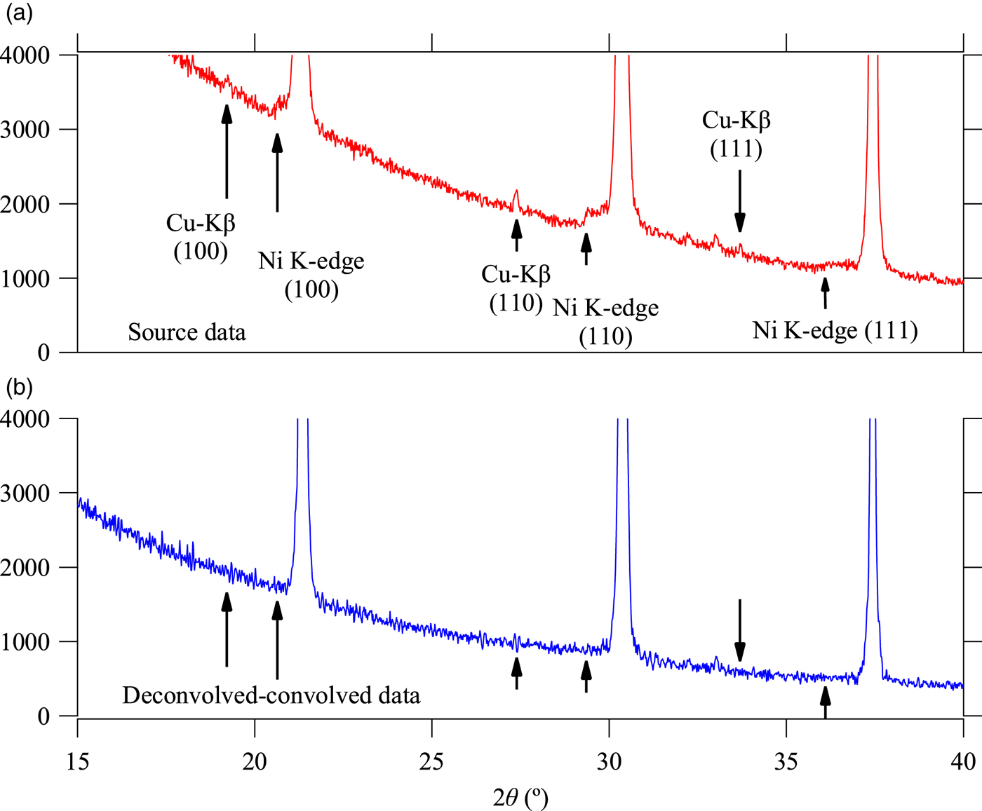
Figure 5. Background intensity profile of the (a) observed and (b) deconvolved–convolved data in lower diffraction angle range.
There still remains ambiguity to determine the parameters to characterize the observed white X-ray profile, x 0, I B, x B, and Δx B, which should be dependent on the extinction of the X-ray and/or sensitivity of the detector, rather than the intrinsic spectroscopic profile of bremsstrahlung. We have assumed x B = 0.17 and Δx B = 0.48 based on the simulation of the extinction by air through the total beam path of 480 mm in length, as described in Section II B, and neglected the absorption of beryllium window and sensitivity of the detector. The value of integrated intensity of the white X-ray, assumed to be I B = 0.4, effectively reduces the step structure caused by NiK-absorption edge, as can be seen in Figure 5(b), but it should also be dependent on the values of x B and Δx B.
Figure 6 shows the spectroscopic profile of f X:Ni(x) and f X*:Ni*(x) used for deconvolution and convolution, respectively. The profile f X:Ni(x) includes the contribution of the white X-ray, but the profile f X*:Ni*(x) does not include white X-ray (f B = 0). It should be noted that the step structure caused by NiK-edge absorption is primarily because of the white X-ray and the contribution of the tails of Kα emission peak intensities at the points of NiK-absorption edge is not large. Since there is no restriction for the hypothetical profile model f X*:Ni*(x), a more appropriate model may be derived, if a more realistic model for the spectroscopic profile of white X-ray is known.
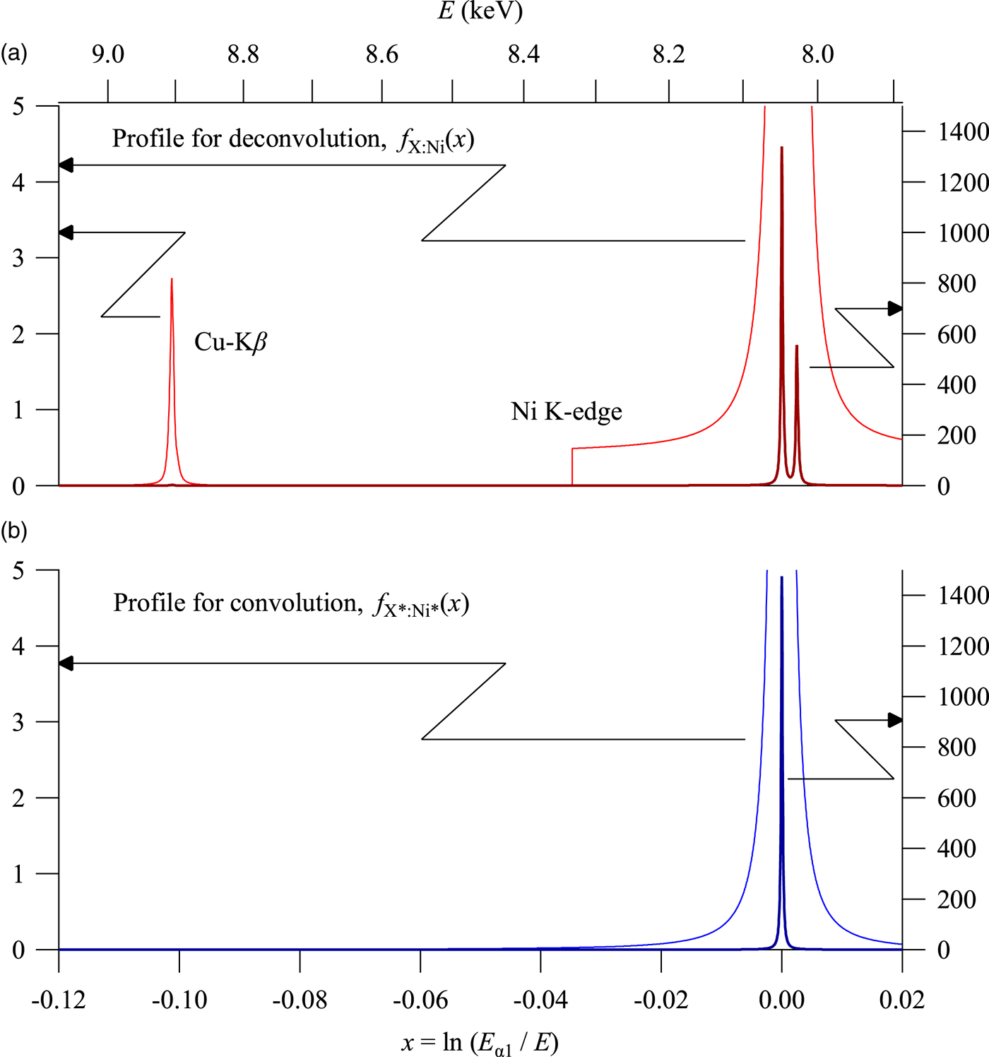
Figure 6. Spectroscopic profile used for (a) deconvolution and (b) convolution.
The deconvolution–convolution treatment looks advantageous particularly for the data measured with a Ni-foil Kβ-filter. The treatment can also simplify subsequent analysis, such as individual peak profile fitting or whole pattern fitting, because of the smoothened background and the Kα 1 singlet peak profile, the latter of which will be simulated by a simple profile function.
The use of a convolved (FPA) peak profile model (Cheary and Coelho, Reference Cheary and Coelho1992) may still be an alternative to the deconvolution–convolution method, but the application of the FPA method to individual peak profile fitting will become more restricted, if the CuKβ or NiK-edge structures in the observed intensity profile cannot be neglected.
V. CONCLUSION
Powder diffraction intensity data of standard LaB6 powder measured with CuKα X-ray source and Ni-foil Kβ filter have been treated by a deconvolution–convolution method based on the abscissa-scale transform and Fourier transform calculations. A CuKα quartet model with asymmetric Kα 1 and Kα 2 peak profiles, and a CuKβ quintet model have been incorporated in the model on the deconvolution, and a hypothetically symmetric Kα 1 singlet profile has been applied on the convolution. There still remains ambiguity for treatment of the contribution of the white X-ray generated by bremsstrahlung, which is necessary to be considered for the removal of NiK-edge structures, but the removal of CuKα 2 and CuKβ peaks is quite straightforward in the theoretical framework of this method.