


1. Introduction
The existence of pollution externalities has been widely acknowledged by scholars and policy makers. Nevertheless, the policy solution is a point of contention. Environmental economists have proposed various policy options including Piguvian tax, pollution permits and abatement activities. While some of these policies have also been employed in developed countries, such policy options may be viewed as visionary concepts in developing countries. Among the most pressing problems developing countries face in dealing with the issue of environment is their limited financial resources. As a result, environmental degradation in developing countries has attracted the attention of policy makers and pundits in developed countries. Headlines such as ‘European Union plans to allocate 15 billion euros per year in environmental aid to poor countries’ (Financial Times, 8 September 2009) are commonly seen in the media.
Anecdotal evidence of foreign environmental aid to developing countries is abundant. The United States donated about US$ 30.5m to developing countries to protect the environment and combat global warming in 1994 alone.Footnote 1 Table 1 shows various environmental protection projects in developing countries that were financed by donations by the European Union (EU) in 2006, totaling 16.5 million euros. The EU also provided African, Caribbean and Pacific (ACP) countries with about €200m in the form of environmental aid in 2009.Footnote 2 Vietnam alone received a total of US$ 144m from Australia, Denmark and the Netherlands for water sanitation, climate change and marine protection projects. Therefore, whether pollution emitted by developing countries is local or global, foreign environmental aid plays a crucial role. Nevertheless, foreign aid alone is not sufficient. It will have to be coupled with a national emission control policy. This paper is an attempt to study the dynamics of pollution control and the effects of foreign environmental aid on the economies of developing countries.
Table 1. Environmental aid by European Union to developing countries in 2006

Source: EU Press Release (2006).
The literature on economic environmental policies is extensive and goes back to the pioneering works of Crocker (Reference Crocker and Wolozin1966) and Baumol (Reference Baumol1971). We briefly review three branches of literature that are most close to our work. First, numerous authors have considered various emission control policies (for example, see Crocker, Reference Crocker and Wolozin1966; Baumol, Reference Baumol1971; Baumol and Oate, Reference Baumol and Oates1988; Long, Reference Long1992; Chao and Yu, Reference Chao and Yu2000; Hatzipanayotou et al., Reference Hatzipanayotou, Lahiri and Michael2005, Reference Hatzipanayotou, Lahiri and Michael2008; Ishikawa and Kiyono, Reference Ishikawa and Kiyono2006; and more recently Mukherjee et al., Reference Mukherjee, Dijkstra and Mathew2011, among others). The second branch of literature which is related to our work focuses on pollution abatement activities and includes Khan (Reference Khan1996), Chao and Yu (Reference Chao and Yu1999), Hadjiyiannis et al. (Reference Hadjiyiannis, Hatzipanayotou and Michael2009) and, more recently, Beladi et al. (Reference Beladi, Liu and Oladi2013). The third branch of literature that our paper contributes to deals with foreign aid tied to environmental cleanup. Chao and Yu (Reference Chao and Yu1999) study the welfare effects of environmental aid. Schweinberger and Woodland (Reference A.G. and Woodland2008) consider the effect of tied on abatement and employment, while Hadjiyiannis et al. (Reference Hadjiyiannis, Hatzipanayotou and Michael2013) study the issue of aid competition and aid fungiblility.Footnote 3 While Chao and Yu (Reference Chao and Yu1999) also derive the conditions under which environmental aid is immiserizing, their setup is static. Nevertheless, the nature of environmental cleanup requires a dynamic framework as in Beladi et al. (Reference Beladi, Liu and Oladi2013). As it will be discussed shortly, our paper incorporates this essential feature.
The purpose of the current paper is to analyze the effect of foreign aid aimed at financing pollution abatement activities in a developing economy in a dynamic general equilibrium framework, given that the government of the developing country pursues an optimal national pollution control policy. To address these effects we consider a Ricardian economy with two goods, a labor-intensive good and a pollution-intensive good. Production of both goods emits pollutants as by-products (this is consistent with the literature). As Khan (Reference Khan1996) noted that abatement in developing countries is more likely to be public rather than private, we also postulate that abatement is a public activity. We further assume that it is financed by foreign aid. In contrast to both Chao and Yu (Reference Chao and Yu1999) and Schweinberger and Woodland (Reference A.G. and Woodland2008), we make a distinction between emission as a flow and pollutant stock as in Beladi et al. (Reference Beladi, Liu and Oladi2013). Hence, our model is dynamic whereas both models in Chao and Yu (Reference Chao and Yu1999) and Schweinberger and Woodland (Reference A.G. and Woodland2008) are static. While some of our results may also be obtained using a static model as in Chao and Yu (Reference Chao and Yu1999), we believe our distinction between emission as a flow and pollution stock is very crucial since many pollutants may take time to be absorbed by nature. In essence, the nature of environmental cleanup implies that a stock of pollution exists. For example, if the aid is tied to abating pollution in a contaminated river, the distinction of emission flow and pollution stock is crucial.
We show that foreign aid tied to pollution abatement increases emission while its effect on pollution stock is ambiguous at the steady-state autarky equilibrium. On the other hand, when the developing economy is a trading economy and is specialized in the production of the pollution-intensive good, such type of aid reduces the steady-state levels of emission and pollution stock. Moreover, under both scenarios the foreign aid can be immiserizing. As stated earlier, we rule out terms of trade effect of aid by assuming a small recipient economy. Thus, the channel through which immiserization takes place is different from previous studies and the literature on neoclassical transfer paradox. In other words, we present a new channel through which aid can be welfare reducing for a recipient country.
Following this introduction, we will present a dynamic general equilibrium model representing our Ricardian developing economy in section 2. Section 3 assumes that a developing economy is closed to international trade and characterizes the steady-state equilibrium and the effects of foreign aid. We then modify our set-up in section 4 and analyze the effects of foreign environmental aid for a small trading developing economy. Section 5 concludes the paper.
2. The model
Assume a Ricardian economy with three sectors: two good sectors and an environmental abatement sector. The good sectors produce a labor-intensive good and a pollution-intensive good, both of which emit pollution as a by-product in Ricardian fashion. As in Beladi and Oladi (Reference Beladi and Oladi2011), production technologies are represented by:
 $$Q_d = \min \lcub \alpha L_d\comma \; \beta E_d\rcub$$
 $$Q_c =\min \lcub \gamma L_c\comma \; \delta E_c\rcub$$
where Q d , Q c , L d , L c , E d and E c are the production of the pollution-intensive sector, production of the labor-intensive sector, labor usage of sector d, labor usage of sector c, emission level for the pollution-intensive good, and emission level for the labor-intensive good, respectively.Footnote 4 Moreover, α, β γ and δ are Ricardian production parameters and all are strictly positive. We assume that α/β > γ/δ, that is good d is pollution intensive while good c is labor intensive.Footnote 5
The public abatement sector employs labor to abate pollution with its production technology given by:
 $$A=A\lpar L_a\rpar $$
where A is the level of abatement and L a is the labor employment by the abatement sector. We assume that A ′ > 0 and A ″ ≤ 0. Assuming full employment of labor, we have:
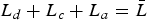 $$L_d+L_c+L_a={\bar L}$$
where
 $\bar L$
is the constant stock of labor. Finally, the total flow of emission, denoted by E, is the sum of emission level by the two good sectors:
$\bar L$
is the constant stock of labor. Finally, the total flow of emission, denoted by E, is the sum of emission level by the two good sectors:
 $$E_d+E_c=E. $$
We postulate that workers (including those employed by the public abatement sector) receive the economy-wide competitive wage. Abatement is financed by foreign aid provided by the north. Therefore, the abatement sector faces the following financing constraint:
 $$wL_a=T $$
where w is the competitive real wage rate in terms of the labor-intensive good and T denotes foreign aid.Footnote 6 The aid enters the resource constraints of the recipient economy in the usual way (see Lahiri, Reference Lahiri2004; Beladi and Oladi, Reference Beladi and Oladi2006). It should also be noted that we assume that aid is indeed used for its intended purposes (that is pollution abatement in our case). However, in some instances aid may be fungible (see Lahiri and Raymondos-Moller, Reference Lahiri and Raimondos-Moller1997; Hadjiyiannis et al., Reference Hadjiyiannis, Hatzipanayotou and Michael2013).Footnote 7
Turning now to the consumption side of the economy, assume that preferences are represented by:
 $$W=u\lpar C_d\comma \; C_c\rpar -f\lpar X\rpar $$
where, C d and C c are consumption of the pollution-intensive and labor-intensive goods, respectively, and X denotes the stock of pollution. We impose the standard neoclassical assumptions on function u, that is, ∂u/∂C d > 0, ∂u/∂C c > 0, ∂2 u/∂C d 2 < 0, ∂2 u/∂C c 2 < 0 and ∂2 u/∂C d ∂C c > 0. We also assume that both goods are normal. Moreover, f(X) is the environmental damage to consumers, where f(0) = f ′(0) = 0, f ′(X) > 0, ∀X > 0, and f ″(X) > 0, ∀ X ≥ 0. That is, marginal environmental damage is zero when there is no pollutant, but it increases at an increasing rate in pollutant stock. This specification of welfare function is consistent with the literature.
The law of motion for pollution stock is given by:
 $$\dot X=E-\sigma X -A\lpar L_a\rpar $$
where
 $\dot X=dX/dt$
and σ ∈ (0, 1) is the natural absorption rate. This motion law states that the rate of change in the pollution stock is equal to the current emission net of what is absorbed by nature and abatement. Making this distinction between emission as a flow and pollution as a stock is very important. Apart from its theoretical curiosity, as stated in the introduction, formulating the dynamics of pollution stock represents many real pollutants such as nuclear waste, and chemical and other industrial wastes. Such pollutants often remain unabsorbed by nature for a long time. Therefore, we need to incorporate the stock of pollution as well as emission flow into our model for such types of pollutants. In our formulation, the natural absorption rate is σ. For short-lived pollutants, σ is close to zero, whereas for pollutants with a long life cycle such as nuclear waste, σ is closer to 1.
$\dot X=dX/dt$
and σ ∈ (0, 1) is the natural absorption rate. This motion law states that the rate of change in the pollution stock is equal to the current emission net of what is absorbed by nature and abatement. Making this distinction between emission as a flow and pollution as a stock is very important. Apart from its theoretical curiosity, as stated in the introduction, formulating the dynamics of pollution stock represents many real pollutants such as nuclear waste, and chemical and other industrial wastes. Such pollutants often remain unabsorbed by nature for a long time. Therefore, we need to incorporate the stock of pollution as well as emission flow into our model for such types of pollutants. In our formulation, the natural absorption rate is σ. For short-lived pollutants, σ is close to zero, whereas for pollutants with a long life cycle such as nuclear waste, σ is closer to 1.
The government, in addition to its abatement activities, chooses an optimal level of emission. Thus, it faces the following control problem
 $$\max_{E} \int_{0}^{\infty} [ u\lpar C_d\comma \; C_c\rpar -f\lpar X\rpar ] exp\lpar -rt\rpar dt $$
 $$s.t. \quad \dot X=E-\sigma X -A\lpar L_a\rpar $$
 $$X\lpar 0\rpar =X_0\comma \; $$
where r ∈ (0, 1) is the discount rate. Note that although the government also manages the abatement activities, the choice abatement level is fully determined by the level of aid through financing constraint.
3. The effects of aid under autarky
We characterize the steady-state equilibrium under autarky in the this section.Footnote 8 In doing this, we start with the production side of the economy, given a level of emission allowed by the government. Since markets are competitive, we conclude from equation (6) that L a = T/γ. This, along with equations (4) and (5), as well as the optimal emission–labor ratios, implies that:
 $$E_d = \displaystyle{{\alpha \delta} \over {\alpha \delta - \gamma \beta}} E -\displaystyle{{\alpha \gamma} \over {\alpha \delta - \gamma \beta}} {\bar L} +\displaystyle{{\alpha} \over {\alpha \delta - \gamma \beta}} T $$
 $$E_c = \displaystyle{{\alpha \gamma} \over {\alpha \delta - \gamma \beta}}{\bar L} -\displaystyle{{\beta \gamma} \over {\alpha \delta - \gamma \beta}}E -\displaystyle{{\alpha} \over {\alpha \delta - \gamma \beta}} T. $$
Since the equilibrium production quantities are given by Q
d
= βE
d
and Q
c
= δE
c
, equations (12) and (13) also determine the equilibrium quantities of production. Finally, as we have C
d
= Q
d
and C
c
= Q
c
+ T under autarky, our general equilibrium is fully determined for a given economy-wide pollution level. Note that the foreign aid is delivered in the form of the labor-intensive good (the numeraire good). By substituting the equilibrium consumption levels in equation (7), we obtain the indirect welfare function
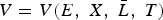 $V=V\lpar E\comma \; X\comma \; \bar L\comma \; T\rpar$
. Therefore, the government's problem will be:
$V=V\lpar E\comma \; X\comma \; \bar L\comma \; T\rpar$
. Therefore, the government's problem will be:
 $$\max_{E} \int_{0}^{\infty} V\lpar E\comma \; X\comma \; \bar L\comma \; T\rpar exp\lpar -rt\rpar dt $$
 $$s.t. \quad \dot X=E-\sigma X -A\left(\displaystyle{{T} \over {\gamma}}\right)$$
 $$X\lpar 0\rpar =X_0. $$
The Hamiltonian for this optimal control problem is given by:
 $$H=V\lpar E\comma \; X\comma \; \bar L\comma \; T\rpar exp\lpar -rt\rpar +\lambda \left[E-\sigma X -A\left(\displaystyle{{T} \over {\gamma}}\right)\right]$$
where λ is the co-state variable. First-order conditions are given by:
 $$\left(\displaystyle{{\partial u} \over {\partial C_d}} \displaystyle{{\partial Q_d} \over {\partial E}} + \displaystyle{{\partial u} \over {\partial C_c}} \displaystyle{{\partial Q_c} \over {\partial E}} \right)exp\lpar -rt\rpar +\lambda=0 $$
 $$\dot \lambda =f^{\prime}\lpar X\rpar exp\lpar -rt\rpar +\lambda \sigma $$
as well as equation (15). We leave the sufficient stability conditions to the appendix. Now, we characterize the steady-state equilibrium of this economy. This equilibrium can be fully characterized by condition
 $\dot X=\dot \lambda =0$
as well as equation (18). That is, using equations (12), (13), (15), (18) and (19), along with
$\dot X=\dot \lambda =0$
as well as equation (18). That is, using equations (12), (13), (15), (18) and (19), along with
 $\dot X=\dot \lambda =0$
, we obtain:
$\dot X=\dot \lambda =0$
, we obtain:
 $$E-\sigma X -A\left(\displaystyle{{T} \over {\gamma}}\right)= 0 $$
 $$f^{\prime}\lpar X\rpar -\displaystyle{{\alpha \beta \sigma \delta} \over {\alpha \delta - \gamma \beta}} \displaystyle{{\partial u} \over {\partial C_d}} + \displaystyle{{\beta \gamma \sigma \delta} \over {\alpha \delta - \gamma \beta}} \displaystyle{{\partial u} \over {\partial C_c}} = 0. $$
By solving equations (20) and (21), we obtain the steady-state equilibrium values of E and X. Let E = ξ (X) and E = ζ (X) denote equations (20) and (21), respectively. By differentiating equation (20) for a given T, we obtain dξ/dX = σ> 0. To calculate the slope of ζ, totally differentiate equation (21) for a given T to obtain:
 $$f^{\prime\prime}\lpar X\rpar dX+\Omega dE=0 $$
where Ω = 2αγ[βσδ/(αδ − γβ)]2(∂2 u/∂C d ∂C c ) − [αβσδ/(αδ − γβ)]2(∂2 u/∂C d 2) − [βσγδ/(αδ − γβ)]2(∂2 u/∂C c 2). It follows from the assumptions we imposed on u and the production functions that Ω > 0. Note that αδ − γβ > 0 since α/β > γ/δ. Therefore, we conclude from equation (22) that dζ/dX = −f ″(X)/Ω < 0. Figure 1 depicts the steady-state equilibrium. We will address all the stability conditions in the appendix.

Figure 1. Steady-state equilibrium
To answer the main question we raised, we conduct comparative dynamics analysis of the equilibrium which allows us to study the effects of environmental aid on steady-state values. By totally differentiating equations (20) and (21) with respect to T, we obtain:
 $$\displaystyle{{dE} \over {dT}} - \sigma \displaystyle{{dX} \over {dT}} = \displaystyle{{A^{\prime}\lpar .\rpar } \over {\gamma}} $$
 $$\Omega \displaystyle{{dE} \over {dT}} + f^{\prime\prime}\lpar X\rpar \displaystyle{{dX} \over {dT}} = \Delta $$
where Δ = [αβσδ/(αδ − γβ)][∂2 u/∂C d ∂C c ] − [(βγσδ)/(αδ − γβ)]∂2 u/∂C c 2 > 0. By solving the above system of equations we obtain:
 $$\displaystyle{{dE} \over {dT}} = \displaystyle{{\sigma\gamma \Delta +A^{\prime}\lpar .\rpar f^{\prime\prime}\lpar .\rpar } \over {\gamma\lpar f^{\prime\prime}\lpar .\rpar +\sigma \Omega\rpar }} $$
 $$\displaystyle{{dX} \over {dT}} = \displaystyle{{\gamma\Delta-\Omega A^{\prime}\lpar .\rpar } \over {\gamma\lpar f^{\prime\prime}\lpar .\rpar +\sigma \Omega\rpar .}} $$
Therefore, we have dE/dT > 0 while the sign of dX/dT is ambiguous. Since we just established that dE/dT > 0, it directly follows from equations (12) and (13) that dQ d /dT > 0 and dQ c /dT < 0, respectively. Hence, we have the following proposition.
Proposition 1
Northern aid to finance abatement in a small southern economy in the absence of trade will result in: (i) an increase in emission in the southern country; (ii) an ambiguous effect on southern pollution stock; and (iii) an increase (decrease) in production of the pollution (labor) intensive good.
Such type of environmental foreign aid increases emission in the developing country and its effects on pollution stock are ambiguous. While the sign of this latter effect is not clear, it is certainly possible that the increased emission outweighs abatement. Thus, foreign environmental aid can increase pollution stock.Footnote 9 That is, foreign aid which is meant to improve environmental degradation in a recipient developing country will paradoxically increase emission and can increase pollution stock. The intuitive explanation of this result is better understood after considering the effects of such type of aid on consumption. For this reason, we postpone presenting our intuitive explanation of this result until we consider the effects of environmental aid on consumption.
Figure 2 shows the effects of an increase in foreign aid. Note from equation (20) that dξ/dT = A ′(.)/γ > 0. That is, an increase in aid shifts this curve upward. To see the effect of foreign aid on ζ, totally differentiate equation (21) with respect to E and T to obtain:

Figure 2. The effects of foreign aid
 $$\displaystyle{{d\zeta} \over {dT}} = \displaystyle{{\Omega} \over {\Delta}} \gt 0. $$
Thus, as an increase in foreign aid shifts ξ up and ζ down, an increase in environmental aid will increase the steady-state level of emission while its effect on pollution stock is ambiguous as stated in Proposition 1. We depicted figure 2 so that the pollution stock increases.
Another interesting issue that arises here is the effect of foreign aid on steady-state levels of consumption of both goods and welfare.Footnote 10 First, we calculate that the consumption of the pollution-intensive good rises since dC d /dT = dQ d /dT > 0 following Proposition 1. Recall from Proposition 1 that production of the labor-intensive good falls. Thus, signing the effect of aid on consumption of the labor-intensive good is not straightforward since aid is delivered in units of this good and we have dC c /dT = dQ c /dT + 1. Now using this as well as equations (13) and (25), we obtain:
 $$\displaystyle{{dC_c} \over {dT}} =-\displaystyle{{\sigma\lpar \gamma\Delta+\alpha\beta\Omega\rpar +\lpar \beta \gamma +A^{\prime}\lpar .\rpar \rpar f^{\prime\prime}\lpar .\rpar } \over {\lpar \alpha \delta -\gamma \beta\rpar \lpar f^{\prime\prime}\lpar .\rpar +\sigma\Omega\rpar }}. $$
It follows from equation (28) and our factor intensity ranking that dC c /dT < 0. To summarize, an increase in environmental aid increases the steady-state production and consumption levels of the pollution-intensive good while it lowers the production and consumption levels of the labor-intensive good. As established earlier, the pollution stock can also increase. Therefore, a decrease in welfare as a result of this type of aid is a possibility. Thus, we have the following result.
Proposition 2
Northern foreign aid to finance abatement in a small southern economy in the absence of trade increases (decreases) the consumption of the pollution (labor) intensive good. Moreover, such type of aid can be immiserizing.
Now we return to an intuitive explanation of Proposition 1. An increase in aid which increases abatement also initially increases the consumption of the labor-intensive good since aid is delivered in the form of the labor-intensive good, ceteris paribus. On the one hand, this leads to an initial increase in the marginal rate substitution of the pollution-intensive good, all else being constant. On the other hand, the discounted weighted marginal utility of goods (that is bracketed terms in equation (20)) will no longer be equal to the shadow price of pollution stock λ. An instantaneous increase in production and consumption of the pollution-intensive good will bring these two components back to equilibrium. This must also lead to a decrease in production of the labor-intensive good as labor moves to the pollution-intensive sector and the abatement sector. Moreover, overall emission must rise due to our pollution intensity ranking. Initially, aid raises the consumption of the labor-intensive good while also causing labor to move to the abatement sector; an increase in production of the pollution-intensive good will also lead to movement of labor from the labor-intensive good sector to the pollution-intensive sector which results in a further decrease in production of the labor-intensive sector. All in all, the overall reduction in the steady-state level of labor-intensive production outweighs the initial increase in consumption of this good due to transfer. Thus, the steady-state level of the labor-intensive good falls. The possibility of immiserizing is somewhat intuitive. As foreign aid increases, the production as well as the consumption of the pollution-intensive good increases. Since we showed that the consumption of the labor-intensive good falls, it is certainly possible that the utility associated with the consumption of goods falls. This alone makes immiserizing aid possible even if the pollution stock falls. Since we showed that a rise in pollution stock is also possible, clearly the immiserizing aid is even more likely under this scenario.
Finally, it should be emphasized that we offer a new channel through which immiserizing aid takes place. Recall that immiserization aid in neoclassical trade theory arises through terms of trade. Here, in this section, the economy is closed to international trade and therefore the terms of trade are irrelevant. Since aid encourages abatement and the abatement production function uses domestic productive resources, foreign aid draws these productive resources away from consumption goods which in turn makes immiserization possible.
4. International trade
In this section we assume that the recipient economy is open to international trade. In addition, we assume that the international price of the pollution-intensive good, denoted by P*, is higher than the autarky equilibrium price of the preceding section, that is P* > γ/α. Thus, the pollution-intensive good is the exportable good for the aid recipient economy and the labor-intensive good is its importable good. It follows from our Ricardian production set-up that Q c = L c = E c = 0 and Q d = α L d = βE d = βE. The budget constraint of the recipient economy is given by P*Q d + T = P*C d + C c , implying a trade balance condition of P*e = m where e = Q d − C d exports of the pollution-intensive good and m = C c − T is imports of the labor-intensive good net of aid.
Having laid out the consumption and production of our set-up under free trade, we now turn to the problem of the government. As in the preceding section, the government chooses the economy-wide level of emission and clean-up. However, as the pollution abatement is fully determined through the financing constraint, this problem reduces to the choice of emission. Thus, the optimal control problem that the government faces is given by:
 $$\max_{E} \int_{0}^{\infty} [ u\lpar \beta E -e\comma \; m+T\rpar -f\lpar X\rpar ] exp\lpar -rt\rpar dt $$
 $$s.t. \quad \dot X=E-\sigma X -A\left(\displaystyle{{T} \over {\gamma}}\right)$$
 $$X\lpar 0\rpar =X_0. $$
The Hamiltonian function for this problem is
 $$\eqalign{H\lpar E\comma \; X\comma \; t\semicolon \; EX\comma \; IM\comma \; T\comma \; \rpar & = [ u\lpar \beta E - EX_d\comma \; IM_c\rpar -f\lpar X\rpar ] exp\lpar -rt\rpar \cr & \quad +\lambda \lpar E-\sigma X -A\left(\displaystyle{{T} \over {\gamma}}\right).} $$
National income in our Ricardian set-up is given by I = P*Q
d
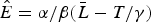
+ T. It directly follows that national income is monotonically increasing in choice of emission given T. Thus, for any given T, H is monotonically increasing in E for all
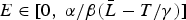 $E\in [ 0\comma \; \alpha/\beta \lpar \bar L -T/\gamma\rpar ]$
since both goods are normal. Therefore, the following equations, as well as equation (32), constitute the first-order conditions for this optimal control problem.
$E\in [ 0\comma \; \alpha/\beta \lpar \bar L -T/\gamma\rpar ]$
since both goods are normal. Therefore, the following equations, as well as equation (32), constitute the first-order conditions for this optimal control problem.
 $$H\lpar \hat E\comma \; X\comma \; m\comma \; T\rpar \ge H\lpar E\comma \; X\comma \; m\comma \; T\rpar \comma \; \quad \forall E\in \left[0\comma \; \displaystyle{{\alpha } \over {\beta }} \lpar \bar L -T/\gamma \rpar \right]$$
 $$\dot \lambda = f^{\prime} \lpar X\rpar exp\lpar -rt\rpar + \lambda X $$
where
 $\hat E = \alpha/\beta \lpar \bar L -T/\gamma \rpar$
.Footnote
11
Equation (33) implies that we have a corner solution. As in the preceding section we are interested in the steady-state equilibrium. As our control variable has a constant time path, at steady state we must have:
$\hat E = \alpha/\beta \lpar \bar L -T/\gamma \rpar$
.Footnote
11
Equation (33) implies that we have a corner solution. As in the preceding section we are interested in the steady-state equilibrium. As our control variable has a constant time path, at steady state we must have:
 $$E=\displaystyle{{\alpha } \over {\beta }}\left(\bar L -\displaystyle{{T} \over {\gamma }}\right)$$
 $$\dot \lambda = f^{\prime} \lpar X\rpar exp\lpar -rt\rpar +\lambda X=0 $$
 $$\dot X = E-\sigma X - A\left(\displaystyle{{T} \over {\gamma}} \right). $$
By solving the above system of equations, we get our steady-state equilibrium:
 $$X = \displaystyle{{1} \over {\sigma}} \left[\displaystyle{{\alpha } \over {\beta }}\left(\bar L -\displaystyle{{T} \over {\gamma}}\right)-A\left(\displaystyle{{T} \over {\gamma}}\right)\right]$$
 $$\lambda =-\displaystyle{{f^{\prime}\lpar X\rpar exp\lpar -rt\rpar } \over {\displaystyle{{1} \over {\sigma}}\left[\displaystyle{{\alpha }\over{\beta}}\left(\bar L -\displaystyle{{T} \over {\gamma}}\right)-A\left(\displaystyle{{T} \over{\gamma}}\right)\right]}}. $$
Note that E is a constant and defined by equation (35). To see the effects of foreign aid, differentiate equations (35), (38) and (40) to obtain: dE/dT = −α/(βγ) < 0 and dX/dT = −1/σ(α/β + A ′(.)/γ) < 0. Then, it directly follows that dQ d /dT = −α/γ < 0. Thus, we have the following results.
Proposition 3
An increase in northern aid to finance abatement in a small southern economy with comparative advantage in production of the pollution-intensive good will reduce emission, the production level of the pollution-intensive good and pollution stock.
To see the reason behind these results, note that the production possibility frontier for the two goods shifts inward as a result of aid. This leads to a decrease in production (of the pollution-intensive good) in the recipient country and emission. Pollution stock falls unambiguously since aid also increases abatement.
Next consider the effects of an increase in aid on national income. By differentiating the equation for national income with respect to aid, we obtain dI/dT = −αP*/γ + 1 < 0 since we assumed that P* > γ/α, that is the recipient country has comparative advantage in the pollution-intensive good. As both goods are normal and the relative price is fixed at the free trade price, consumption of both goods will have to fall. Since the trade balance condition implies that P*e = C c − T, it directly follows that export of the pollution-intensive good also falls. As for the welfare effect of an increase in aid, the utility obtained from consumption of goods falls as we have already established that consumption levels for both goods fall. However, since pollution stock falls as a result of an increase in aid, it reduces pollution damage. Therefore, there are two opposing effects on welfare. On the one hand, the welfare falls since the utility obtained from consumption of goods falls, that is du/dT < 0. On the other hand, the welfare rises due to the reduced pollution damage, that is df/dT = f ′(.)dX/dT = −f ′(.)/[σ (α /β +A ′(.)/γ )] < 0. Thus, we have the following result on welfare.
Proposition 4
Northern aid to finance abatement in a small southern economy with comparative advantage in production of the pollution-intensive good decreases national income. Moreover, it can be immiserizing.
The intuition is straightforward. An increase in foreign aid will lead to a flow of labor from the production sectors to abatement, resulting in a reduction in the production of the good for which our developing country is specialized. This is due to the fact that the production possibility frontier shifts inward as
 $\bar L-L_{a}$
falls. Since both goods are normal and international good prices are fixed, both C
d
and C
c
must fall. This clearly reduces u(.). On the other hand, since an increase in aid will reduce emission and increase abatement activities, X must fall and so must the pollution damage f(X). Therefore, aid will be immiserizing if the former effect outweighs the latter.
$\bar L-L_{a}$
falls. Since both goods are normal and international good prices are fixed, both C
d
and C
c
must fall. This clearly reduces u(.). On the other hand, since an increase in aid will reduce emission and increase abatement activities, X must fall and so must the pollution damage f(X). Therefore, aid will be immiserizing if the former effect outweighs the latter.
It is worth reiterating that the cause of immiserization in our result is different from what is in neoclassical transfer paradox, whereby the negative terms of trade change leads to immiserizing transfer. Here, the terms of trade effect is absent. Basically, the cause of immiserizing aid is that this type of aid is resource using. That is, to use tied aid in abatement, other productive resources that otherwise would be used in production of final goods must be used. Therefore, as a result of an increase in foreign aid, the production function possibility frontier for consumption goods shifts inward since less of the productive resources will be available for production activities. Hence, this is the reason for possible immiserization.
5. Concluding remarks
In this paper we have constructed a dynamic Ricardian general equilibrium model of pollution control, abatement, foreign aid and trade for a small developing economy. The developing economy produces and consumes two goods, a pollution-intensive good and a labor-intensive good. The recipient government employs two policies. On the one hand, it controls the quantity of emission. On the other hand, it conducts pollution abatement activities financed by foreign aid. Although it is noted in policy circles that the developing economies lack the financial resources to deal with the pollution problem and therefore the developed countries should take part by providing these countries with foreign aid to reduce pollution, aid alone is not sufficient. In addition, the governments in these countries should also take charge and have an effective national emission control policy. This has motivated us to incorporate abatement, financed by aid, and national emission control into our analysis. We characterized the steady-state equilibrium both with and without trade. We showed that, while the effects of environmental tied aid on the stock of pollution is ambiguous, it will increase the emission level unambiguously under autarky. Our main conclusion is that such type of aid will fail to reduce emissions while its effect on pollution stock may go either way if the recipient economy is an isolated economy, such as North Korea. Moreover, we illustrated that foreign aid can be immiserizing. Although environmental aid reduces both emission and pollution stock in a recipient economy that has comparative advantage in the pollution-intensive good, its effect on national income is negative and it can be immiserizing.
We have tried in this paper to construct and use a basic and tractable dynamic model to convey our message. Clearly, our analysis can be extended in different directions. First, one can extend our paper to partial domestic financing of abatement activities. As another example, instead of the Ricardian production model, one can use the Heckscher–Ohlin–Samuelson (HOS) model. Using any alternative models, while they may be more realistic but less mathematically tractable, should not change the crux of our ideas that foreign aid to finance public abatement activities is resource using. It is this aspect of foreign aid that may lead to immiserization in developing countries. In particular, as far as H-O-S type models are concerned, our conjecture is that one can impose assumptions on production structure such that special cases like factor intensity reversal do not take place. Thus, one can view labor in our formulation as the labor–capital ratio (that is labor per unit of capital). We conjecture that under this extension our main results remain the same. Again, the reason is that with this extension aid remains as resource using which is a distortion that may result in immiserization. Possible extension of our paper is not limited to alternative modeling choice. Our paper can be extended by considering alternative fundamental assumptions. For example, one can use our set-up to study the effects of foreign environmental aid received by a large developing economy, notwithstanding that aid recipients are small and poor developing counties. Another, and perhaps more interesting extension is to use our formulations and investigate the effects of private abatement in a developing economy financed by foreign investment. Finally, one can consider a case where foreign environmental aid is fungible.
Appendix: Equilibrium stability
We first consider the stability conditions for the autarky case in this appendix. Rewrite equation (18) as:
 $$\lambda=\psi \lpar E\rpar $$
where ψ(E) = −(βδ/(αδ − γβ))(α∂u/∂C d − γ∂u/∂C c )exp(−rt). Differentiate this equation; use equations (12) and (13) and market clearing conditions to obtain:
 $$\psi^{\prime}\lpar E\rpar =-\left(\displaystyle{{\alpha\beta\delta} \over {\alpha\delta-\gamma\beta}}\right)^2\displaystyle{{\partial^2u} \over {\partial C_d^2}} -\left(\displaystyle{{\beta\gamma\delta} \over {\alpha\delta-\gamma\beta}}\right)^2\displaystyle{{\partial^2u} \over {\partial C_c^2}} \geq 0. $$
Let ϕ(λ) be the inverse of ψ. It follows from the implicit function theorem and equation (41) that dE/dλ = 1/ψ′ > 0. Now, substitute ϕ(λ) in equation (15) and rewrite the system of differential equations (15) and (19) as:
 $$\dot X = \phi\lpar \lambda\rpar -\sigma X -A\lpar .\rpar $$
 $$\dot \lambda = f^{\prime}\lpar X\rpar exp\lpar -rt\rpar +\sigma \lambda. $$
Linearize the above system and let J be the Jacobian matrix of the linearized system. It is easy to verify that trace (J) = 0 and |J| = −σ2 − ϕ′(.)f
″(.)exp(−rt) < 0 as we already established that ϕ′(.) > 0. Thus, it follows that the characteristic roots are real with the opposite sign, concluding that the equilibrium is a saddle point. Therefore, it is enough to show that the transversality condition is met to guarantee the stability of our steady-state equilibrium. However, this is satisfied since it follows from equation (40) that
 $\lim_{t\rightarrow \infty}\lambda=\lim_{t\rightarrow \infty}\psi\lpar .\rpar =0$
.
$\lim_{t\rightarrow \infty}\lambda=\lim_{t\rightarrow \infty}\psi\lpar .\rpar =0$
.
Next consider the free trade steady-state equilibrium of section 4. Note that emission has a constant time path. Use equation (35) to re-write the differential equation (37) as:
 $$\dot X+\sigma X=\Theta $$
where
 $\Theta=\lpar \alpha/\beta\rpar \lpar \bar L-T/\gamma\rpar -A\lpar .\rpar$
. The solution to this differential equation is X(t) = Θ/σ + κ exp(-σt), where κ is the integrating constant. Clearly, X(t) is convergent.
$\Theta=\lpar \alpha/\beta\rpar \lpar \bar L-T/\gamma\rpar -A\lpar .\rpar$
. The solution to this differential equation is X(t) = Θ/σ + κ exp(-σt), where κ is the integrating constant. Clearly, X(t) is convergent.


