2. SIGNAL OPTIONS

There are two fundamental ways in which the two BOC signals can be combined, as shown in Figure 4; these are known as CBOC (Composite BOC) and TMBOC (Time-Multiplexed BOC). In both cases, 1/N of the power is in the BOC(6,1) component. Note that it is not a requirement that N is an integer, nor that the BOC(6,1) part of the TMBOC signal is every Nth chip; in practice, a less regular multiplexing scheme would be used. For example, Hein, Betz et al (Reference Hein and Betz2006) suggest that the BOC(6,1) chips could be the 1st, 5th, 7th and 30th of every 33.

Figure 4. CBOC and TMBOC.

In the CBOC approach, the two BOC components are simply added together, while in the TMBOC approach, they are sent for different chips of the spreading code. Furthermore, there is the choice to be made whether the BOC(1,1) and BOC(6,1) signals both start with a value of +1 (as shown in Figure 1), or whether the latter is inverted; this is here referred to as the phase of the BOC(6,1) component (with the term in phase meaning that both signals start with a +1). Whereas with TMBOC the BOC(1,1) and BOC(6,1) signals are sent in different time intervals, and so do not interact, this is not the case with CBOC, and this gives rise to some interesting properties in both the time and frequency domains. Firstly, there is marked effect on the signal spectrum, as shown in Figure 5, with the anti-phase case having the greater high-frequency energy.

Figure 5. Spectra for In phase and Anti-phase CBOC

Secondly, although the BOC(1,1) waveforms and BOC(6,1) waveforms as shown in Figure 1 have zero cross-correlation for zero time offset, this is no longer true when the signal is band-limited, as shown in Figure 6. It may be seen that the cross-correlation is greatest at narrow bandwidths; as will be shown later, this results in a change in the correlation loss for such receivers, according to the phase of the BOC(6,1) signal, with the in phase case having the greater correlation, i.e. the lower loss.

Figure 6. Cross-correlation between BOC(6,1) and BOC(1,1).

In the light of the above, it is clear that only a limited number of choices will give the desired MBOC spectrum; three of these are:

• • ¾ of the power in the pilot signal, using TMBOC with 4/33 of the chips modulated by BOC(6,1). The remaining ¼ of the power is in the data signal, which uses BOC(1,1). This is the proposed solution for GPS L1C.

• • ½ of the power in the pilot signal, using CBOC with the BOC(6,1) component in anti-phase, and ½ of the power in the data signal, using CBOC with the BOC(6,1) component in-phase. In both cases, the CBOC signal has 10/11 of its power in the BOC(1,1) component and 1/11 in the BOC(6,1) component. This will be referred to as the CBOC option for Galileo.

• • ½ of the power in the pilot signal, using TMBOC with 2/11 of the chips modulated by BOC(6,1) in-phase, and ½ of the power in the data signal, using BOC(1,1) modulation. This will be referred to as the TMBOC option for Galileo.

The remainder of this paper will be concerned with the last two of these options. They were chosen from a wider initial range on their performance and the feasibility of their implementation within Galileo. A direct comparison against the first (GPS) option is difficult, because of the effect of the different power split between data and pilot signals.

There are many ways in which the signal waveform may affect the navigation performance, but here three of the most significant, and most easily understood, are considered: correlation SNR loss, RMS bandwidth and multipath performance. Since many low-cost receivers will simply track the BOC(1,1) part of the signal, this approach is considered as well as that of a receiver matched to the transmitted waveform. Similarly, the options of tracking just the pilot signal, and tracking both data and pilot, are both addressed. The following three sections are devoted to these performance measures.

3. CORRELATION SNR LOSS

Correlation loss is a measure of the reduction in amplitude of the correlation peak from the ideal case. This can result from bandwidth limitation (in satellite or receiver), the use of a mismatched reference signal in the receiver, or (not considered here) signal distortion. Correlation loss has an impact primarily on data demodulation (since it reduces the post-correlation SNR) and acquisition.

While correlation loss measures the reduction in correlation peak amplitude through the effects of receiver mismatch to the transmitted signal and band limitation, it is also true that these factors affect the response of the correlator to noise. Of course, this effect cancels out when comparing the response of the same receiver to different signals, but is significant when comparing the performance of different receivers to the same signal. To evaluate the effects on both signal and noise, it is more convenient to work in the frequency domain.

Suppose that the received signal has a spectrum S(f) and the receiver local reference has a spectrum R(f). Furthermore, suppose that the receiver has a brickwall filter of bandwidth B and that the noise density at the receiver input is N ₀. Then the signal and noise output powers of the receiver (punctual) correlator, when tracking, are given by:

(2)

For the TMBOC case, the integrals are evaluated separately for the BOC(1,1) and BOC(6,1) parts of the signal, and then summed with the appropriate weighting. If we normalise the signal power (in infinite bandwidth) and noise spectral density to unity, the ratio P _S/P _N gives the loss in SNR at the correlator output, relative to a matched receiver of infinite bandwidth. Subtracting the corresponding value for the baseline BOC(1,1) signal then gives the additional SNR loss due to the choice of signal and receiver.

Figure 7 shows the results of this calculation for the pilot component of both signals and the data component of the CBOC signal, over a wide range of receiver bandwidths. (The data component of the TMBOC signal uses BOC(1,1) modulation, and so is not plotted as the additional loss is clearly zero.) A number of interesting points are apparent. Taking the CBOC case first:

• • For very narrow receiver bandwidths, BOC and matched receivers perform the same for any given signal. This is because, viewed in that bandwidth, the reference signal spectrum in both cases differs only in magnitude, and inspection of the equations for signal and noise power reveals that (as expected) this cancels out.

• • For very wide receiver bandwidths, the losses with a matched receiver tend to zero.

• • For very wide receiver bandwidths, with a BOC receiver, the additional loss tends to the fractional power loss in the BOC(1,1) component (i.e. 10/11 or 0·41 dB).

• • The loss is lower when the BOC(6,1) component is in-phase (i.e. the data component) and higher when it is in anti-phase (i.e. the pilot component), with this effect decreasing with increasing receiver bandwidth. This is because of the non-zero cross-correlation between filtered BOC(6,1) and BOC(1,1), as already noted.

For the TMBOC case:

• • For very narrow receiver bandwidths, the loss is the same with either a matched receiver or a BOC receiver with blanking (i.e. where the correlator is disabled for the BOC(6,1) parts of the signal). This is because the noise reaching the correlator during the BOC(6,1) periods has no energy in the region of the peaks of the BOC(6,1) reference spectrum, and so does not degrade the SNR.

• • With a BOC receiver using blanking, the additional loss is equal to the fractional power loss in the BOC(1,1) component (i.e. 9/11, or 0·83 dB), independent of the receiver bandwidth. This is because, while the correlation peak is reduced (in linear terms) by the square of this amount, blanking also reduces the noise by 9/11.

• • For very wide receiver bandwidths, with a BOC receiver without blanking, the additional loss tends to twice the fractional power loss in the BOC(1, 1) component (i.e. 1·66 dB).

Figure 7. Additional Correlation SNR Loss.

The conclusion is that, while the CBOC and TMBOC options perform similarly with a matched receiver, the CBOC option suffers less loss when used with a BOC(1,1) receiver; furthermore, if TMBOC is used with a BOC(1,1) receiver, then failure to implement blanking introduces a significant further loss.

4. RMS BANDWIDTH

The RMS or Gabor bandwidth of a signal, as normally defined, is a measure of the second derivative of its normalised autocorrelation function at the origin. In the case of a matched receiver (i.e. with a reference identical to the incoming signal), this determines the relative code tracking accuracy (for a given SNR) in an AWGN channel (Woodward, Reference Woodward1953).

When considering a non-matched receiver (for example, when a BOC receiver is used with a CBOC or TMBOC signal), the standard definition must be modified slightly. If the received signal is x(t), with Fourier transform X(f), the reference signal is y(t), with Fourier transform Y(f), and the receiver bandwidth B (assumed less than the transmitted bandwidth, with a brickwall response), then the effective RMS bandwidth will be defined as:

(3)

This can only be considered valid if the integrals are real-valued, but this is the case with the signals under consideration. Where tracking of both data and pilot components (and/or the non-overlapping parts of TMBOC) is considered, the XY* terms are evaluated separately for both components and then summed.

The results for a matched receiver are shown in Figure 8; the term P refers to tracking of the pilot alone, and D+P to tracking both data and pilot. It is clear from Equation 3 above that the RMS bandwidth is a function of just the signal spectrum, and hence those cases that have the same spectrum (for the component(s) being tracked) have the same RMS bandwidth; thus, in particular, when data and pilot are both tracked, both CBOC and TMBOC signals have the same RMS bandwidth. Below 10 MHz receiver bandwidth, most of the BOC(6,1) component is filtered out, and hence all signals perform the same; above that, the greater the fraction of BOC(6,1) in the signals being tracked, the wider the RMS bandwidth. However, both the CBOC and TMBOC signals show significant benefits compared against BOC(1,1).

Figure 8. RMS Bandwidth (Matched Receiver).

The effective RMS bandwidth with a BOC(1,1) receiver is shown in Figure 9. Note that the results for TMBOC are without blanking; if blanking is used, then it is clear that the effective RMS bandwidth is identical to that of BOC(1,1). The same comments as above apply, but the differences are much smaller. When data and pilot are both tracked, the CBOC case is identical to the BOC(1,1) baseline, because all cross-correlation terms cancel. It is worth noting that the CBOC case, with tracking of the pilot alone, gives a better RMS bandwidth than for a BOC(1,1) signal, even with a BOC(1,1) receiver.

Figure 9. Effective RMS Bandwidth (BOC(1,1) receiver).

5. MULTIPATH

The modulation performance in the presence of multipath propagation depends mainly on the waveform autocorrelation profile, and therefore the receiver bandwidth, and the discriminator function and correlator spacing used. Multipath error performance results and comparisons for the proposed MBOC modulations in terms of error envelopes, cumulative running average errors or mean error against correlator spacing for different multipath channels can be found in (Hein et al, Reference Hein2006; Artaud et al., Reference Artaud2007; Hoult, Aguado and Crescimbeni, Reference Hoult, Aguado and Crescimbeni2006). From these results we can observe a clear advantage in multipath performance from the MBOC spectrum over BOC(1,1), with small differences between the candidate MBOC modulations.

Earlier multipath performance results in the project were derived in simplified simulations through manipulation of the signal correlation function for a desired multipath channel and receiver code and carrier loop models. A lower level validation of these results and comparison of the modulations in realistic scenarios was desired, accounting for any non-linear receiver effects occurring in a detailed sample-level receiver simulation. For this purpose, the Leeds University receiver emulation was used to compare the performance of the CBOC and BOC modulations in a realistic scenario. This software receiver replicates at sample level the baseband processing and loop control processes in a hardware high-performance GNSS receiver with channel bandwidth B=24 MHz and correlator spacing d=0·1 chip. The high-resolution aeronautical channel model developed by Steingass et al. (Reference Steingass2004) has been used to generate realistic multipath channel profiles. Only the CBOC modulation has been chosen, due to the processing length of the simulations. A model of the environment producing such multipath is shown in Figure 10. This model corresponds to an aircraft approach descending at a constant rate towards the runway with a small period of taxiing on the ground. The Matlab software provided by DLR was used to generate each of the multipath components over the course of the approach. It contains the direct LOS path; the antenna diffractive path, short-delay fuselage refracted and reflected rays, and the ground reflection component. The model was generated from a combination of physical optics measurements and measurement campaigns for two representative aircraft types.

Figure 10. Realisation view of the channel model. (from Steingass et al., Reference Steingass2004)

The Doppler spread measured for each of the identified paths is small (see Figure 11). This translates to high correlation between samples in the model for a given simulated approach. Since the model is stochastic, a large number of approaches need to be simulated in order to obtain enough independent samples for each operating region model, as determined by the aircraft approach height. Considering the high-resolution of the multipath channel (R _S=1·5 ns to isolate the first independent path in the model) and approach duration (~240 s – plus the initial receiver settling period removed –, start altitude of 800 m, descent rate of 3 m/s plus 20 s taxiing), a multipath simulation carried out on a modern standard desktop PC took 3–4 days of computation time. Therefore, for this study we conducted 64 simulations for each of the two signal types. The measurements suggest that 64 simulations are enough to show meaningful results. The multipath generator Markov models were configured as in the example provided in the documentation provided with the DLR model implementation tuned for the aircraft used during their measurement campaign, with 25·4 Hz sampling rate. The parameters for the channel model are given in Table 1.

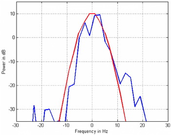
Figure 11. Doppler spectrum of ground reflection after vertical speed correction. (from Steingass et al., Reference Steingass2004)

Table 1. Multipath model parameters from Steingass et al., Reference Steingass2004.

The simulation results under multipath conditions have been differentiated against a corresponding line-of-sight AWGN-only simulation to isolate the effect of the multipath. We have aggregated the results of 64 trials in order to show some of the statistical properties of the model and the receiver performance under this signal modulation. In Figure 12, 64 overlaid traces corresponding to the differentiated receiver code tracking error results for CBOC are plotted. Since the ground reflection delay ranges from near one code chip duration (1 μs) to practically zero delay, the contribution of this component covers most of the multipath error envelope. The code tracking error displays a similar profile of troughs and crests characterising the single specular multipath channel due to the relative weight of the ground reflection. A one to one comparison against a single reflector envelope is not possible because of the different power, statistical nature of the multipath components and the compounded effect of the three multipath components.

Figure 12. CBOC multipath code tracking error for 64 approaches.

In Figure 13(left) the code tracking error measurements within 1-second bins from the 64 simulation trials have been averaged to generate an estimate of the mean tracking error. A consistent very small negative offset can be observed that is probably caused by the non-symmetrical relationship between 0 deg and 180 deg phase multipath envelope, since the channel model path phase distributions are zero mean and there is a reflector at short delay, where the negative multipath error envelope has a slightly higher magnitude. The mean value and standard deviation of the plot in Figure 13(left) are:

In Figure 13(right) all the code tracking error measurements within 1-second bins from the 64 simulation trials have been used to calculate a standard deviation value per bin. The standard deviation has been provided to get an idea of the distribution of the error when compared to the maximum measured errors in Figure 12. A similar pattern to the error envelopes can also be observed for the limited number of independent observations. The maximum σ measured is ~1·4×10⁻³ chip=0·4 m. This is slightly over an order of magnitude lower than the highest peak error (~18×10⁻³ chip=5·3 m).

Figure 13. Mean (left) and standard deviation (right) of CBOC code tracking error for 64 approaches.

We were requested to compare the performance of the CBOC modulation to the BOC(1,1) baseline. For this purpose, the multipath channel models for the same 64 approaches have been used for simulation with the BOC(1,1) signal. As before, in Figure 14, 64 traces of the multipath-only receiver code tracking error are plotted. Again, since the ground reflection delay covers a whole chip of delay ranges, we can see, to the extent allowed by the limited number of results, a similar pattern to the well-known BOC(1,1) multipath error envelope. As expected, the amplitude of the maximum errors is slightly higher than in the CBOC case. This is most noticeable at the longer ground reflection delays. Similar error ratios between BOC and CBOC can be seen for example in (Hoult, Aguado and Crescimbeni, Reference Hoult, Aguado and Crescimbeni2006).

Figure 14. BOC(1,1) multipath code tracking error for 64 approaches.

In Figure 15(left), all the code tracking error measurements within 1-second bins from the 64 simulation trials have again been averaged to generate an estimate of the mean tracking error. A consistent small negative offset can again be observed, in this case larger than for the CBOC modulation. The mean value and standard deviation of the plot in Figure 15(left) are: μ(BOC(1,1))=−2·7205×10⁻⁵ chip, σ(BOC(1,1))=2·6096×10⁻⁵ chip. For the BOC(1,1) modulation, the mean error is 66% greater than CBOC, and the standard deviation is 131% greater.

Figure 15. Mean (left) and standard deviation (right) of BOC code tracking error for 64 approaches.

In Figure 15(right), all the code tracking error measurements within 1-second bins from the 64 simulation trials have been used to calculate a standard deviation value per bin. The standard deviation of the error confirms that the CBOC modulation performs better in terms of the multipath error than the BOC(1,1) modulation in this realistic composite scenario. The maximum σ measured is ~1·6×10⁻³ chip=0·5 m which is only slightly higher than for CBOC. However, the multipath error at most points throughout the approach is significantly higher than for CBOC. The maximum σ peak error is again slightly over an order of magnitude lower than the highest peak error (~21×10⁻³ chip=6·16 m).