2.1. The three-step method to detect cycle slip

The first step of the proposed method involves linearly independent detection of the amount of cycle slip, which is achieved by combining two EWL code–phase and one GF phase combination. Then, the ionospheric delay variation is predicted using the preceding observation sequence without cycle slip, which is used to correct the GF combined observations. Finally, the EWL and the corrected GF combination are used to detect and repair the cycle slip.

Based on the theory of the triple-frequency combination, the combinational observations of phase and code can be described as follows (Richert and El-Sheimy, Reference Richert and El-Sheimy2007; Cocard et al., Reference Cocard, Bourgon, Kamali and Collins2008; Urquhart, Reference Urquhart2009; Yao et al., Reference Yao, Gao, Wang, Hu and Li2016):

(1)$$\begin{align} \lambda_{ijk}\varphi_{ijk}&=\rho-\lambda_{ijk}N_{ijk}+T+\delta_{orb}-\eta_{ijk}I_1+cdt_{ijk}+B_{ijk}+\lambda_{ijk}\varepsilon_{ijk}\label{eq1} \end{align}$$

(2)$$\begin{align}R_{abc}&=\rho+T+\delta_{orb}+\eta_{abc}I_1+cdt_{abc}+b_{abc}+\varepsilon_{abc}\label{eq2}\\ \eta_{ijk}&=\lambda_{ijk}/\lambda_1(i+j\lambda_2/\lambda_1+k\lambda_3/\lambda_1)\notag\\ \eta_{abc}&=a+b(\lambda_2/\lambda_1)^2+c(\lambda_3/\lambda_1)^2\notag\\ \varepsilon_{ijk}&=i\varepsilon_1+j\varepsilon_2+k\varepsilon_3,\varepsilon_{abc}=ae_1+be_1+ce_3\notag \end{align}$$

where φ _ijk and R _abc are the combinational carrier phase (unit: cycles) and code (unit: m) observations, respectively, subscripts i, j and k are integers that are not all zero, and a, b and c are real numbers, where a = b = c = 1/3 adopted here is to minimise the impact of code noise. The combinational ambiguities $N_{ijk}=iN_{1}+jN_{2}+kN_{3}$ and N ₁, N ₂ and N ₃ are the ambiguities of the three frequencies. The combinational wavelength $\lambda_{ijk}=\lambda_{1}\lambda_{2}\lambda_{3}/(i\lambda_{2}\lambda_{3}+j\lambda_{1}\lambda_{3}+k\lambda_{1}\lambda_{2})$, where λ₁, λ₂ and λ₃ are the wavelengths of the three frequencies. Furthermore, T is the tropospheric delay, δ_orb represents satellite orbit errors, I ₁ is the ionospheric delay of the B1 frequency, η_ijk and η_abc are ionospheric influence coefficients of the combinational phase and code, respectively, cdt _ijk and cdt _abc are clock errors of the combinational phase and code, respectively, B _ijk and b _abc are hardware delays of phase and code combinations, respectively, $\varepsilon_{ijk}$ and $\varepsilon_{abc}$ represent the noise of the phase and code combinations, respectively and ε and e represent the noise of the original frequency phase and code, respectively.

Based on the above equations, in adjacent epochs, the epoch difference $\Delta N_{ijk,abc}$ of the combinational code–phase observations can be formulated as:

(3)$$\begin{align} \Delta N_{ijk,abc}&=(\Delta R_{abc}/\lambda_{ijk}-\Delta \varphi_{ijk})-\eta_{ijk,abc}\Delta I_1-(\Delta\varepsilon_{abc}/\lambda_{ijk}-\Delta \varepsilon_{ijk})\label{eq3}\\ \eta_{ijk,abc}&=(\eta_{abc}+\eta_{ijk})/\lambda_{ijk}\notag \end{align}$$

where Δ denotes the single difference in the adjacent epochs and $\eta_{ijk,abc}$ is the ionospheric influence coefficient of the combinational code–phase observations. Most errors can be eliminated or greatly reduced by the single difference in adjacent epochs, such as orbit error, clock error, tropospheric delay and multipath errors. As seen in Equation (3), ρ, T and δ_orb can be eliminated, while other errors can be reduced considerably. In addition, the cycle–slip value is affected both by the ionosphere and by noise. When a code–phase combination with a larger wavelength is adopted, we can ignore the influence of noise on the cycle–slip value. Furthermore, the effect of ionospheric delay can be reduced by selecting a small influence coefficient, particularly for low-sampling-rate observations or highly active ionospheric conditions. Without consideration of the influence of ionospheric delay, the cycle–slip value can be rewritten as follows:

(4)$$\Delta N_{ijk,abc}=(\Delta R_{abc}/\lambda_{ijk}-\Delta \varphi_{ijk})-(\Delta \varepsilon_{abc}/\lambda_{ijk}-\Delta \varepsilon_{ijk})$$

From Equation (4), it is evident that because of the large noise of the code observations, the combinational wavelength has considerable impact on the Standard Deviation (STD) of the cycle–slip value. Therefore, the combinational wavelength is the most important parameter, followed in descending order by the combinational coefficient and the ionospheric influence coefficient. For details on the best code–phase combinations, the reader is referred to Richert and El-Sheimy (Reference Richert and El-Sheimy2007) and Urquhart (Reference Urquhart2009). Here, consistent with Yao et al. (Reference Yao, Gao, Wang, Hu and Li2016), the optimal code–phase combinations of (0, 1,−1) and (1,−5, 4) are employed as the first and second detectable cycle–slip amounts.

Zhao et al. (Reference Zhao, Sun, Dai, Hu, Shi and Liu2014) introduced an NL combination as a third detectable cycle–slip amount to ensure linear independence of the three employed amounts. In contrast from this strategy, Yao et al. (Reference Yao, Gao, Wang, Hu and Li2016) introduced a GF phase combination to ensure mutual independence. Both methods correct the third detectable amount using the predicted ionospheric delay based on previous observations, which is because the ionospheric delay has the greatest impact on the NL code–phase combination or the GF phase combination. Moreover, both methods were used to solve the cycle–slip value Δ N ₃ and for rounding purposes. Although the two methods employ the third different cycle–slip detectable amount, we believe the difference between the two methods is negligible.

Consistent with Yao et al. (Reference Yao, Gao, Wang, Hu and Li2016), the following GF phase combination is adopted:

(5)$$\begin{aligned} L_{\alpha\beta\gamma}&=\alpha\lambda_1\varphi_1+\beta\lambda_2\varphi_2+\gamma\lambda_3\varphi_3=-N_{\alpha\beta\gamma}-\eta_{\alpha\beta\gamma}I_1+\varepsilon_{\alpha\beta\gamma}\\ N_{\alpha\beta\gamma}&=\alpha\lambda_1N_1+\beta\lambda_2N_2+\gamma\lambda_3N_3\\ \eta_{\alpha\beta\gamma}&=\alpha\lambda_1+\beta\lambda_2^2/\lambda_1+\gamma\lambda_3^2/\lambda_1\\ \varepsilon_{\alpha\beta\gamma}&=\alpha\lambda_1\varepsilon_1+\beta\lambda_2\varepsilon_2+\gamma\lambda_3\varepsilon_3 \end{aligned}$$

where $L_{\alpha\beta\gamma}$ is the GF phase combinational observation (unit: m) and subscripts α, β and γ are the combinational coefficients. To eliminate the impact of geometrical distance, troposphere delay and satellite orbit error, let $\alpha+\beta+\gamma=0$. Parameters $N_{\alpha\beta\gamma}$, $\eta_{\alpha\beta\gamma}$, $cdt_{\alpha\beta\gamma}$, and $\varepsilon_{\alpha\beta\gamma}$ are the combinational ambiguity, ionospheric amplification factor (different from the ionospheric influence coefficient η_abc), clock errors and noise of the GF phase combinational observation, respectively. In adjacent epochs, the detectable cycle–slip value $\Delta N_{\alpha\beta\gamma}$ of the GF phase by epoch difference can be resolved as follows:

(6)$$\Delta N_{\alpha\beta\gamma}=-\Delta L_{\alpha\beta\gamma}-\eta_{\alpha\beta\gamma}\Delta I_{1}+\Delta \varepsilon_{\alpha\beta\gamma}$$

It can be seen from Equation (6) that the accuracy of the GF detectable cycle–slip value is affected mainly by the deviation value of the combinational ionospheric delay and stochastic noise. Due to the smaller amount of noise associated with phase combinational observations, the most important factor is the ionospheric delay. Thus, because the ionospheric delay has the greatest influence on the GF observation, it has to be corrected by the prediction model when ionospheric delay is greater than the threshold value (for example, 41·9 mm). It is important to note that the combinational ionospheric delay variance $\eta_{\alpha\beta\gamma}\Delta I_{1}$ (replaced by ION in this paper, which is the slant ionospheric delay variance of the GF phase combination) predicted and corrected in this paper is not the ionospheric delay variance of the B1 frequency. Therefore, the combinational ionospheric delay can be minimised by selecting a small ionospheric amplification factor for the prediction and correction model. The prediction model of ionospheric delay variance can be expressed as follows:

(7)$$\eta_{\alpha\beta\gamma}\Delta I_1^k=f(\eta_{\alpha\beta\gamma}\Delta I_1^{k-m},\ldots,\eta_{\alpha\beta\gamma}\Delta I_1^{k-1})$$

where f(…) denotes the mapping function of the ionospheric delay. Here, superscript k denotes the current epoch location and superscript m denotes the number of epochs needed to reflect the ionospheric delay variance rates (the size of window). As previous epochs have no cycle slip, we can obtain the preceding ionospheric delay sequence for the prediction of the subsequent ionospheric delay. In contrast to Chang et al. (Reference Chang, Xu, Yao and Wang2018), to eliminate or greatly reduce the influence of the geometric part, geometric distance, tropospheric delay, satellite orbit, and satellite clock, and to improve the accuracy of the estimated ionospheric delay, the following equation is constructed to solve the preceding ionospheric delay sequence and to both predict the ionospheric delay variance and repair cycle slip in the next epoch:

(8)$$\begin{align}\label{eq8} &\left[\begin{matrix} \lambda_1\Delta\varphi_1-\lambda_2\Delta\varphi_2-\lambda_1\Delta N_1+\lambda_2\Delta N_2\\ \lambda_1\Delta\varphi_1-\lambda_3\Delta\varphi_3-\lambda_1\Delta N_1+\lambda_3\Delta N_3 \end{matrix}\right]\notag\\ &\quad =\left[\begin{matrix} -1+\lambda_2^2/\lambda_1^2\\[3pt] -1+\lambda_3^2/\lambda_1^2 \end{matrix}\right]\Delta I_1+\left[\begin{matrix} \Delta\xi_1+\Delta\xi_2\\ \Delta\xi_1+\Delta\xi_3 \end{matrix}\right]=\textbf{\textit{A}}\Delta I_1+\Delta\xi \end{align}$$

where Δ N ₁, Δ N ₂, and Δ N ₃ are the cycle–slip values of the three frequencies and Δ I ₁ is the ionospheric delay variance of the B1 frequency. In summary, two code–phase combinations and one GF combination are employed to solve the original cycle–slip value, and the resolving equation is constructed as follows:

(9)$$\begin{align} \textbf{\textit{BX}}&=\textbf{\textit{L}}\label{eq9}\\ \textbf{\textit{B}}&=\left[\begin{matrix} i_1 & j_1& k_1\\ i_2 & j_2& k_2\\ \alpha\lambda_1 &\beta\lambda_2 &\gamma\lambda_3 \end{matrix}\right],\quad \textbf{\textit{X}}=[\begin{matrix}\Delta N_1 & \Delta N_2 & \Delta N_3\end{matrix}]^{\rm T}, \quad \textbf{\textit{L}}=[\begin{matrix}n_1 & n_2 & n_3\end{matrix}]^{\rm T}\notag\\ n_1&=\hbox{round}(\Delta N_{(1,-1,0)}),\quad n_2=\hbox{round}(\Delta N_{(1,-5,4)}),\quad n_3=-\Delta L_{\alpha\beta\gamma}^k-\eta_{\alpha\beta\gamma}\Delta I_1^k\notag \end{align}$$

where round(·) denotes direct rounding. Because the STD of the selected code–phase combination is so small that the success rate of rounding is >99·99% (Yao et al., Reference Yao, Gao, Wang, Hu and Li2016), we can regard n ₁ and n ₂ as correct. Compared with the selected code–phase combination, the observational accuracy of the GF combination is weak because of the influence of the ionospheric delay. In short, the accuracy of an unknown cycle–slip value depends mainly on that of the modified ionospheric delay. Through calculation and analysis based on Equation (9), it can be concluded that: the ionospheric delay variance Δ I ₁ of the B1 frequency must be <41·9 mm to ensure correct rounding of the cycle slip with the corresponding value of ION <28·2 mm (ignoring the impact of observed noise).

The cycle slip value X of the triple-frequency original carrier observations can be obtained using Equation (9). As the rounding success rate of the EWL combinations is >99·99%, we can ignore the impact of the EWL combinations on the estimated original carrier cycle slip. Therefore, the original carrier cycle–slip value is affected only by the residual errors of the GF combined observations, which is why we adopted the simplest form of integer rounding. If a higher success rate were desired, the integer least-squares method could be adopted (Teunissen, Reference Teunissen2002).

The original phase observations generate cycle slip as follows:

(10)$$n_1\neq\ 0 \hbox{ or }n_2\neq\ 0 \hbox{ or }\Delta N_3\neq\ 0$$

where n ₁, n ₂ and Δ N ₃ are the three detectable cycle–slip amounts.

2.2. Prediction models for ionospheric delay

There are many prediction models for time series data. Considering the ionosphere delay associated with the variation of satellite elevation angle and the slow variation in sequential epochs, four representative prediction models are employed to test the accuracy of the ionospheric delay predictions: the Sliding Window Mean (SWM) method, Weighted SWM (WSWM) method, Polynomial Fitting (PF) method, and Kalman Filtering (KF) method.

First, when the satellite elevation angle varies slowly or there is a small sampling interval (for example, 1 s), the variation of ionospheric delay can be ignored. In such cases, the SWM model could represent an efficient method. However, for larger sampling intervals (for example, 30 s), the variation of ionospheric delay could be reasonably large, meaning the sliding window constitutes the optimal strategy. Second, because ionospheric delay varies rapidly with time, introducing the WSWM method could provide fuller consideration of the trend by adding a weighted factor for the predicted epoch according to the interval between the sampling point and the predicted point. Third, when the ionospheric delay varies linearly or nonlinearly, the PF method can simulate the variational process based on the least squares method. The PF method is the one used most commonly. For example, the parabolic method, Lagrangian fitting and exponential smoothing are all approximations of the PF method. The PF method can replace other methods when applied to a local area. In addition, the widely used total electron content rate method (Liu, Reference Liu2010) can be considered as an example of the PF method that uses just three sampling points. Finally, the KF method can be used as a representative fitting method to predict ionospheric delay with consideration of process noise.

2.2.1. Sliding Window Mean (SWM) method

Because of the real-time processing required to detect and repair cycle slip, we selected several previous epochs without cycle slip to estimate ION, rather than use a similar forward and backward moving window averaging method. Given that no cycle slip existed before this epoch, we can accurately reflect the ionospheric delay variance rates and trends as follows:

(11)$$\eta_{\alpha\beta\gamma}\Delta I_1^k=f(\eta_{\alpha\beta\gamma}\Delta I_1^{k-m},\ldots,\eta_{\alpha\beta\gamma}\Delta I_1^{k-1})=\frac{1}{m}\sum_{i=1}^m\eta_{\alpha\beta\gamma}\Delta I_1^{k-i}$$

It should be noted that the size of the sliding window (called m) has a certain impact on the accuracy and therefore it cannot be too large or too small; here, we adopted a value of about 20.

2.2.2. Weighted Sliding Window Mean (WSWM) method

As ionospheric delay varies rapidly with time, introducing a weighted method can include consideration of the trend of ionosphere delay more fully by adding a weighted factor for the predicted epoch according to the interval between the sampling point and the predicted point.

In considering the trend of change of ionospheric delay for Inclined Geosynchronous Satellite Orbit (IGSO) and Medium Earth Orbit (MEO) satellites, a weighting factor is employed to construct the WSWM as follows:

(12)$$\eta_{\alpha\beta\gamma}\Delta I_1^k=f(\eta_{\alpha\beta\gamma}\Delta I_1^{k-m},\ldots,\eta_{\alpha\beta\gamma}\Delta I_1^{k-1})=\frac{2}{m+1}\sum_{i=m}^1\,\frac{i}{m}(\eta_{\alpha\beta\gamma}\Delta I_1^{k-(m-i+1)})$$

2.2.3. Polynomial Fitting (PF) method

Existing studies have shown that slant ionospheric delays of IGSO and MEO satellites are mostly parabolic in form with a decrease of satellite elevation angle. Furthermore, a parabolic model can adequately capture the temporal variation of ionospheric delay. The k-th epoch ionospheric delay can be expressed as the following equation:

(13)$$\kappa(t)_{k}=\theta_0+\theta_1t_k+\theta_2t_k^2$$

where κ denotes the k-th epoch slant ionospheric delay ION, θ is the parabolic coefficient, and t is the time interval. Only the second-order PF need be employed because its accuracy is adequate. The ionospheric delay of m epochs can be expressed as:

(14)$$\boldsymbol{\kappa}=\boldsymbol{\tau}\boldsymbol{\vartheta}$$

where $\boldsymbol{\kappa}=\left[\begin{smallmatrix} \kappa_{1}\\ \vdots\\ \kappa_{m} \end{smallmatrix}\right]$, $\boldsymbol{\tau}=\left[\begin{smallmatrix} 1&t_{1}&t_{1}^{2}\\ \vdots & \vdots & \vdots \\ 1&t_{m}&t_{m}^{2} \end{smallmatrix}\right]$, and $\boldsymbol{\vartheta} = \left[\begin{smallmatrix} \theta_{0}\\ \theta_{1}\\ \theta_{2} \end{smallmatrix}\right]$. The estimated parameter $\boldsymbol{\vartheta}$ can be calculated based on the previous m epochs using the following equation:

(15)$$\boldsymbol{\vartheta}=(\boldsymbol{\tau}^{\rm T}\boldsymbol{\tau})^{-1}\boldsymbol{\tau}^{{\rm T}}\boldsymbol{\kappa}$$

2.2.4. Kalman Fitting (KF) method

To ensure the accuracy of the dynamic model, the time difference ionospheric delay, and its velocity and accelerated velocity are employed to construct the KF method (Chang et al., Reference Chang, Xu, Yao and Wang2018). The prediction process is shown as follows:

(16)$$\begin{align} \bar{\textbf{\textit{x}}}_k&=\textbf{\textit{F}}\hat{\textbf{\textit{x}}}_{k-1}\label{eq16} \end{align}$$

(17)$$\begin{align} \bar{\textbf{\textit{P}}}_k&=\textbf{\textit{F}}\hat{\textbf{\textit{P}}}_{k-1}\textbf{\textit{F}}^{T}+\textbf{\textit{Q}}_{k-1}\label{eq17} \end{align}$$

where $\textbf{\textit{F}}=\left[\begin{smallmatrix} 1&t&\frac{t^{2}}{2}\\ 0&1&t\\ 0&0&1 \end{smallmatrix}\right]$, $\boldsymbol{x}=\left[\begin{smallmatrix} \kappa\\ \dot{\kappa}\\ \ddot{\kappa} \end{smallmatrix}\right]$, and $\textbf{\textit{Q}}_{k-1}=\sigma_{\Delta \scriptsize\dddot{\kappa}}^{2}\left[\begin{smallmatrix} \frac{t^{5}}{20} &\frac{t^{4}}{8} & \frac{t^{3}}{6}\\ \frac{t^{4}}{8}&\frac{t^{3}}{3} & \frac{t^{2}}{2}\\ \frac{t^{3}}{6} & \frac{t^{2}}{2} & t \end{smallmatrix}\right]$. Here, x is the estimated parameter, and κ, $\dot{\kappa}$, and $\ddot{\kappa}$ are the value, velocity, and accelerated velocity of the epoch difference ionospheric delay, respectively. The overbar denotes the predicted parameter, $\hat{\textbf{\textit{x}}}$ denotes the estimated parameter, P is the covariance matrix, and Q denotes the observed noise.

The update process is shown as follows:

(18)$$\begin{align} \hat{\textbf{\textit{x}}}_k&=(\textbf{\textit{A}}^{{\rm T}}\tilde{\textbf{\textit{Q}}}_k^{-1}\textbf{\textit{A}})^{-1}\textbf{\textit{A}}^{{\rm T}}\tilde{\textbf{\textit{Q}}}_k^{-1}\textbf{\textit{y}}_k\label{eq18} \end{align}$$

(19)$$\begin{align} \hat{\textbf{\textit{P}}}_k&=(\textbf{\textit{A}}^{{\rm T}}\tilde{\textbf{\textit{Q}}}_k^{-1}\textbf{\textit{A}})^{-1}\label{eq19} \end{align}$$

where $\textbf{\textit{y}}_{k}=\left[\begin{smallmatrix} \bar{\textbf{\textit{x}}}_{k}\\ \boldsymbol{\kappa}_{k} \end{smallmatrix}\right]$ and $\textbf{\textit{A}}=\left[\begin{smallmatrix} 1&0&0\\ 0&1&0\\ 0&0&1\\ 1&0&0\end{smallmatrix}\right]$. In contrast to Chang et al. (Reference Chang, Xu, Yao and Wang2018), ignoring the effects of relevance, $\tilde{\textbf{\textit{Q}}}_{k}=\left[\begin{smallmatrix} \bar{\textbf{\textit{P}}} & 0\\ 0 & \sigma_{\kappa}^{2} \end{smallmatrix}\right]$. It should be noted that this combines the prediction by treating it as a virtual observation, and the ionospheric delay of the current epoch is used to construct the new observations.

To minimise the effect of the current epoch on the observed noise, and to reflect the continuity and trend of the variation of ionospheric delay, a memory factor is introduced as follows:

(20)$$\boldsymbol{\sigma}_{\scriptsize\dddot{\kappa}}^{2}=(1-\mu)\sigma_{\scriptsize\dddot{\kappa}}^2+\mu\hat{\sigma}_{\scriptsize\dddot{\kappa}}^2$$

where μ is the memory factor used to balance the current and previous epoch ionospheric delays.

3.1. Correlation of ionospheric delay and satellite elevation angle

Due to the different operating speeds of the various BDS orbital satellites, three types of satellite data were analysed independently to assess the statistical accuracy of the ionospheric delay and the rounding error of cycle slip. In addition, because the slant ionospheric delay is sensitive to satellite elevation angle, we segmented the time series data based on elevation angle thresholds.

Figure 1 shows the time series of the epoch difference ionospheric delay and elevation angle. It is evident that the ionospheric delay variation of satellite C01 is stable because the elevation angle of GEO satellites remain largely unchanged. However, the ionospheric variation of satellite C11 can be sufficiently large that its effect on the accuracy of the GF combination must be considered. In particular, the ionospheric variation could reach the decimetre level when the elevation angle is <30°. The prediction accuracy of the ionospheric correction directly determines the success rate of rounding cycle slip. In addition, the noise of slant observations will begin to increase sharply (Gerdan, Reference Gerdan1995). Therefore, four types of prediction model were employed and the threshold of the segmentation process was set at 30°.

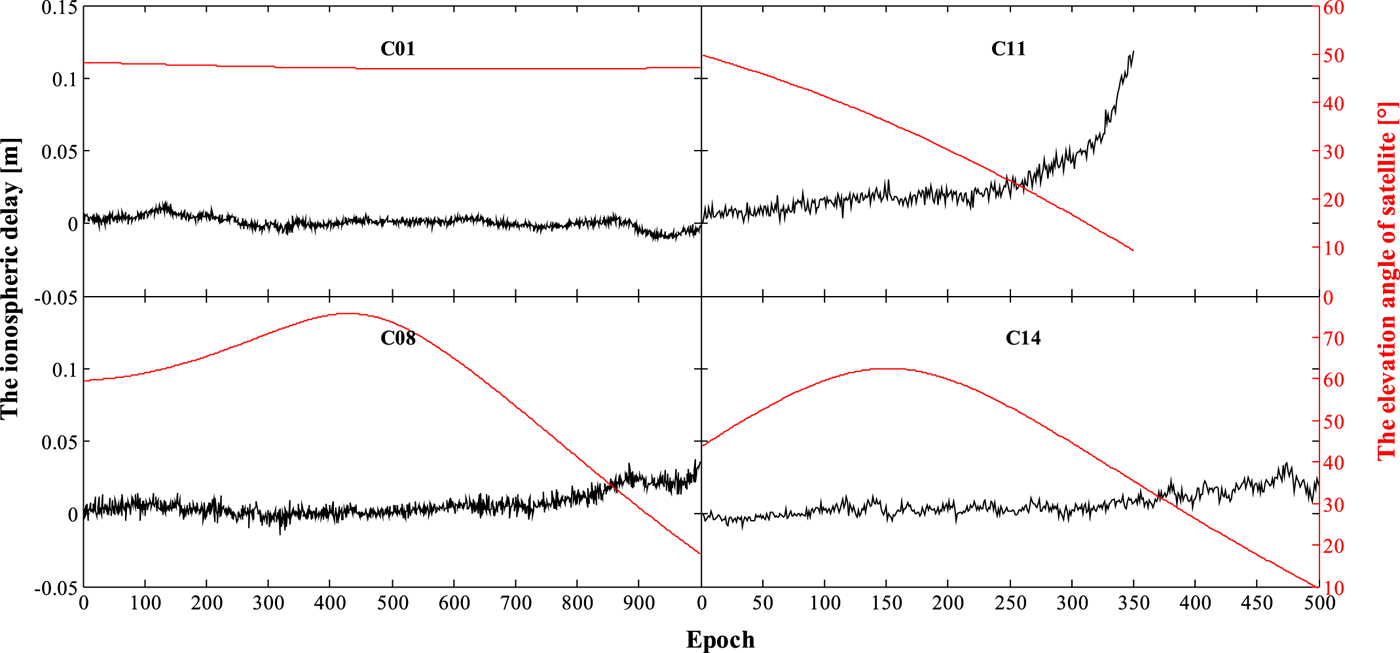
Figure 1. Epoch difference ionospheric delay and elevation angle.

3.2. Statistical accuracy of EWL combination observations

The traditional experiment is to add a certain cycle–slip value to the original data in different epochs and then to use the employed model to detect and repair the cycle slip. However, this strategy is too inefficient and it cannot be used for evaluation in each epoch. More importantly, we found the accuracy of cycle–slip repair depended only on the observed data noise and the employed model. In the analysis, the following three statistics are used: mean (reflecting the effectiveness after ionospheric delay correction), maximum (reflecting whether the cycle–slip estimation is correct), and STD (reflecting the overall accuracy of cycle–slip repair).

The rounding errors of EWL combination float estimations, including the mean, maximum, and STD, are shown in Table 1. It is apparent that the rounding error STD of EWL₁ and EWL₂ for GEO satellites is 0·028 and 0·054 cycles, respectively. Such minor rounding errors have negligible impact on the cycle–slip estimation. In contrast to the GEO satellites, the corresponding STD for IGSO and MEO satellites is 0·07 and 0·09 cycles, respectively. The reason is that the ionospheric delay of GEO satellites is small, while that of IGSO and MEO satellites can be large, even up to the decimetre level, which affects the rounding accuracy of EWL combinations. Fortunately, the overall STD is still so small that the success rate remains >99·999997% (Li et al., Reference Li, Verhagen and Teunissen2014). It should be noted that because of the large wavelength of the EWL combinations, we have not corrected the EWL observations using the previous ionospheric delay. To improve the EWL rounding accuracy further, we should bring Equation (8) into Equation (3) to correct the estimated cycle–slip value using the calculated ionospheric values.

Table 1. Rounding error of EWL float estimations (unit: cycles).

The statistical results are displayed as histograms in Figure 2 for the three selected satellites, that is, C01, C08 and C11. The rounding errors of the cycle–slip estimators follow Teunissen's distribution (Teunissen, Reference Teunissen2002). It is evident that the STD increases gradually in the order of GEO to IGSO and then to MEO satellites; however, the success rate remains close to 100%.

Figure 2. Histograms of EWL rounding error: (top left) C01 EWL₁, (bottom left) C01 EWL₂, (top middle) C08 EWL₁, (bottom middle) C08 EWL₂, (top right) C11 EWL₁, and (bottom right) C11 EWL₂.

3.3. Comparison of prediction model accuracy for GEO satellites

In contrast to EWL combinations, NL combinations have a smaller wavelength and therefore the effect of ionospheric delay on the observation must be taken into account. Four improved prediction models were used to predict the ionospheric delay and the rounding accuracy (fractional deviation) of Δ N ₃ for each of the GEO satellites is presented in Table 2. It is evident that the STD is mostly <0·06 cycles, with an average value of 0·046 cycles, for which the corresponding rounding success rate is close to 100%. In addition, the prediction accuracies of the SWM and WSWM methods are slightly higher than the PF and KF methods. The main reason is that the ionospheric delay of GEO satellites is more stable over reasonably short periods, despite a certain degree of volatility. Therefore, we did not segment the accuracy statistics for GEO satellites.

Table 2. Rounding accuracy of ΔN ₃ for GEO satellites (unit: cycles).

Note: Bold font indicates preferred results.

The predictions of ionospheric delay for the GEO satellites derived from the four prediction models are shown in Figure 3. It can be seen that all four models produce a reasonable smoothing effect and that they are effective in overcoming the noise of the estimated ionospheric delay.

Figure 3. Estimated ionospheric delay and predicted values of the four models for satellite C01.

The differences between the predicted ionospheric values and the estimated values from the four improved prediction models for the C01 satellite are shown in Figure 4. It is apparent that the differences remain generally unchanged (that is, mostly within a range of 5 mm), which could both ensure high accuracy of the GF combination after ionospheric delay correction and ensure the accuracy of the repaired cycle slip.

Figure 4. Difference between the estimated ionospheric delay and predicted values of the four prediction models for the C01 satellite: (top left) SWM, (top right) WSWM, (bottom left) PF, and (bottom right) KF.

3.4. Comparison of prediction model accuracy for IGSO and MEO satellites

As described in Section 3.1, we segmented the data for IGSO and MEO satellites and set the satellite elevation angle threshold to 30°. Tables 3 and 4 present the rounding accuracy of Δ N ₃ of the four prediction models for satellite elevation angles >30° and <30°, respectively.

Table 3. Rounding accuracy of ΔN ₃ for IGSO and MEO satellites for elevation angles >30°(unit: cycles).

Note: Bold font indicates preferred results.

Table 4. Rounding accuracy of ΔN ₃ for IGSO and MEO satellites for elevation angles <30° (unit: cycles).

Note: Bold font indicates preferred results.

For satellite elevation angles >30°, the statistical accuracies of IGSO and MEO satellites are consistent with GEO satellites, and the SWM and WSWM methods are slightly better than the PF and KF methods (Table 3). This is mainly because ionospheric delay variation is small when the elevation angles of IGSO and MEO satellites are >30°. Therefore, using windowing and simple averaging is most stable and reliable. Moreover, the STD of the Δ N ₃ rounding error is always <0·07 cycles. Considering that the rounding success rate of the EWL₁ and EWL₂ combinations is >99·999997%, the results obtained using the prediction models in this paper suggest the final rounding success rate of BDS triple-frequency cycle slips is close to 100%.

Conversely, for satellite elevation angles <30°, the SWM model performs slightly better in comparison with the other models (Table 4). Even though the accuracy of ION prediction declines slightly, the STD of Δ N ₃ rounding errors is <0·1 cycles (Teunissen and de Bakker, Reference Teunissen and de Bakker2013), which ensures the rounding success rate of BDS triple-frequency observations is close to 100%.

Figures 5 and 6 show the ionospheric delay variation for the C08 and C11 satellites, respectively, based on the four improved prediction models. It can be seen that the maximum ionospheric delay variations of the C08 and C11 satellites reach 40 and 120 mm, respectively. Moreover, if ionospheric delay correction is not performed, the estimation of cycle slip will be incorrect, which will result in failure of the cycle–slip repair.

Figure 5. Estimated ionospheric delay and predicted values of the four prediction models for satellite C08.

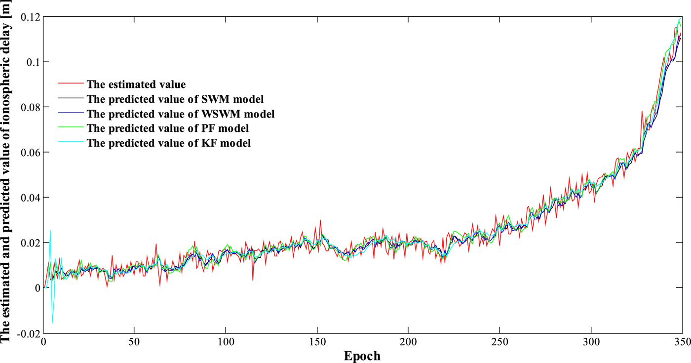
Figure 6. Estimated ionospheric delay and predicted values of the four prediction models for satellite C11.

Figures 7 and 8 display the differences between the estimated ionospheric delay and the predicted values of the four prediction models for the C08 and C11 satellites, respectively. It is evident that as satellite elevation changes, the difference fluctuates considerably, especially when the satellite elevation angle is <30°. However, most of the ionospheric delay variation is within a range of 10 mm, which can ensure the rounding success rate of cycle–slip estimation is close to 100%. In addition, there is little difference between the four improved prediction models.

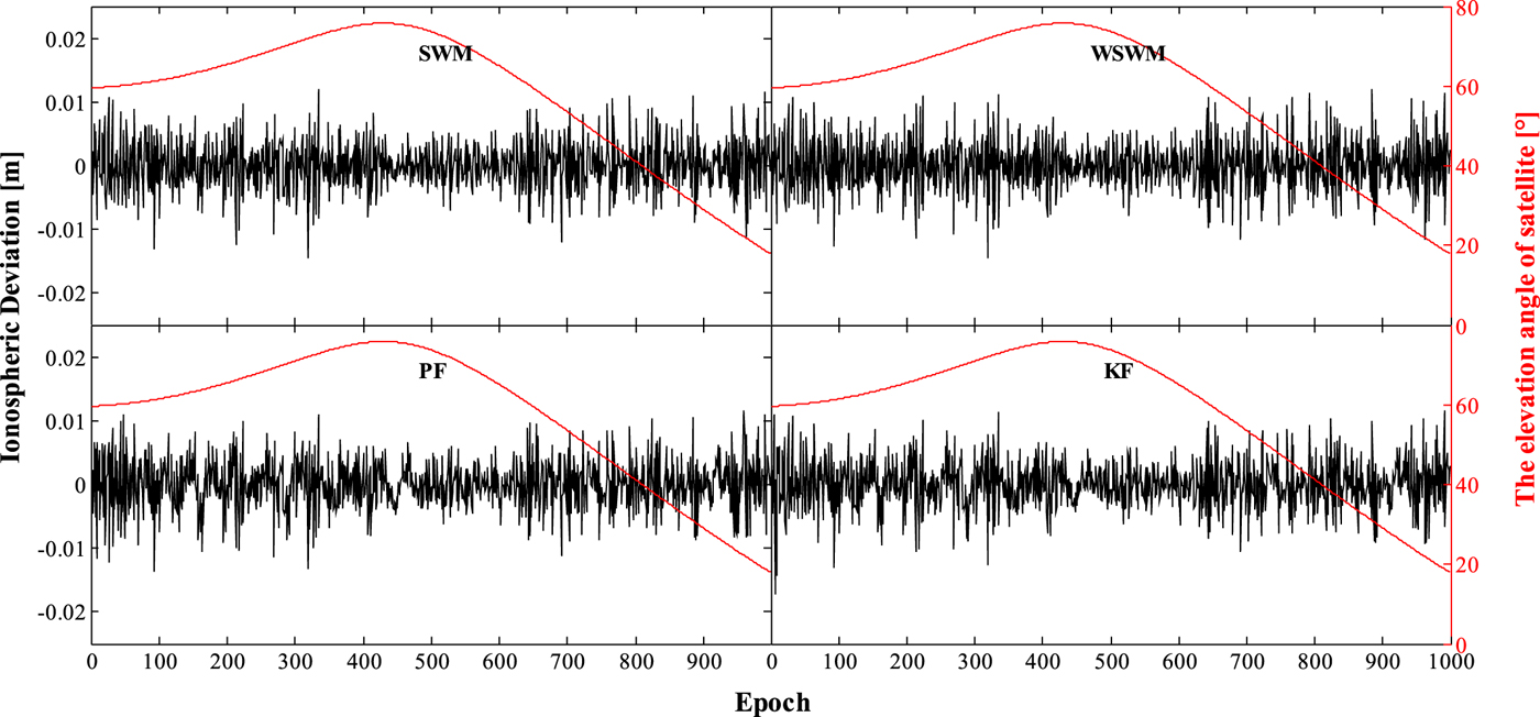
Figure 7. Difference between the estimated ionospheric delay and predicted values of the four prediction models for the C08 satellite: (top left) SWM, (top right) WSWM, (bottom left) PF, and (bottom right) KF.

Figure 8. Difference between the estimated ionospheric delay and predicted values of the four prediction models for the C11 satellite: (top left) SWM, (top right) WSWM, (bottom left) PF, and (bottom right) KF.

3.5. The results of cycle slip detection and repair

To illustrate the efficiency of cycle–slip detection and repair, Figures 9(a)-(c) show the rounding errors of the estimates of EWL₁, EWL₂, and Δ N ₃ for the C01, C08 and C11 satellites, respectively. The rounding errors of Δ N ₃ for the C08 and C11 satellites are shown in Figures 9(b) and 9(c), respectively, based on the improved prediction models (the SWM, as an example, ignores the differences among the different models). It can be seen that the maximum rounding error of Δ N ₃ for the C08 and C11 satellites is 0·6 and 2·0 cycles (or 40 and 120 mm), respectively. If the residual ionospheric delay corrections were not performed, the estimation of cycle slip would be incorrect, resulting in failure of the cycle–slip repair. Compared with Chang et al. (Reference Chang, Xu, Yao and Wang2018), the use of the ionospheric prediction models in this paper ensures the rounding accuracy of Δ N ₃ is equivalent to that of EWL₁ and EWL₂. Thus, it is shown to be effective in improving the overall accuracy of cycle–slip repair.

Figure 9. Test values of cycle–slip detection. (a) Satellite C01. (b) Satellite C08. (c) Satellite C11.

In addition, no case was found in Figures 9(a)-(c) where the cycle–slip detection amount was >0·5 cycles, after correcting the residual ionospheric delay, which means the cycle–slip repair was all correct in this data processing.

3.6. Cycle slip detection and repair under high ionospheric activity

To verify the effectiveness of the four models in repairing cycle slip under conditions of high ionospheric activity, data from station SHA1 obtained on 26 August 2018 was used for analysis. The sampling interval was 30 s and the period of observation was 23 h (data for the final hour was missing). The ionospheric delay on this day was active and the corresponding Kp index reached a value of seven. The corresponding ionospheric delay variation is shown in Figure 10. Compared with the values obtained during the stable ionosphere period (Figures 3, 5 and 6), Figure 10 shows the ionospheric delay variation of station SHA1 on 26 August 2018 was more active, with the value for many satellites reaching 2–4 cm.

Figure 10. The ionospheric delay variation of station SHA1 on 26 August 2018.

The rounding errors of EWL combination float estimations are shown in Table 5. Compared with Table 1 (ionosphere not active), the STD is no larger and all values are <0·09 cycles, except for the C05 satellite (corresponding satellite elevation angles range from 14°–16°); however, the maximum of EWL₂ has a large increase. This is primarily due to the active ionospheric variance and shorter wavelength of EWL₂. However, as can be seen from the maximum values, the rounding values of EWL combinations were acceptable for all satellites and all epochs.

Table 5. Rounding error of EWL combination under high ionospheric activity (unit: cycles).

The rounding accuracy of Δ N ₃ for all GEO satellites is presented in Table 6. On the one hand, it is evident that the STD has been greatly increased (up to 0·064 cycles) in comparison with that derived under conditions with a stable ionosphere. Moreover, the C05 satellite has an epoch cycle–slip repair error due to the lower satellite elevation angle (15°), and the maximum deviation of Δ N ₃ was >0·5 cycles. On the other hand, the experimental results show the accuracies of the SWM and KF methods were higher, while the performance of the PF method was worse.

Table 6. Rounding accuracy of ΔN ₃ for GEO satellites under high ionospheric activity (unit: cycles).

Note: Bold font indicates preferred results; italic font indicates failure of cycle–slip repair.

We segmented the data for IGSO and MEO satellites and set the satellite elevation angle threshold to 30°. Tables 7 and 8 present the statistical accuracies of the four prediction models for satellite elevation angles >30° and <30°, respectively. For satellite elevation angles >30°, the STD of the Δ N ₃ rounding error had a small increase (up to 0·58 cycles). However, there was no incorrect rounding of Δ N ₃ for any of the satellites in all epochs. In addition, the experimental results show the accuracies of the SWM and KF methods were higher, while the performance of the PF method was worse.

Table 7. Rounding accuracy of ΔN ₃ for IGSO and MEO satellites for elevation angles >30° under high ionospheric activity (unit: cycles).

Note: Bold font indicates preferred results.

Table 8. Rounding accuracy of ΔN ₃ for IGSO and MEO satellites for elevation angles <30° under high ionospheric activity (unit: cycles).

Note: Bold font indicates preferred results; italic font indicates failure of cycle–slip repair.

For satellite elevation angles <30°, it is evident from the maximum values that cycle–slip repair failed for several satellites (for example, C06, C11 and C14), mainly because of the large ionospheric variation. In addition, the experimental results show the SWM and KF methods were superior for IGSO and MEO satellites, respectively.

To clarify the effect of adding the correction value for ionospheric delay and the effect of cycle–slip repair using the four models, Table 9 shows the statistics of cycle–slip detection and repair for all satellite observations. The results show the ionospheric delay correction can greatly improve the success rate of cycle–slip repair (that is, an improvement from 98·411% to 99·993%). Moreover, it is found that failure of cycle–slip repair occurs continually when the satellite elevation angle is <30°. This is considered attributable mainly to large variation of the ionospheric delay, which means it is necessary to correct the residual ionospheric delay.

Table 9. Results of cycle-slip repair under high ionospheric activity.