3.1. Coarse-grained mechanics

We follow Moreau et al. (Reference Moreau, Giraldi and Gadêlha2018), stating the governing equations of elasticity for this slender inextensible unshearable filament in pointwise form as

(3.1)\begin{gather} \boldsymbol{n}_s - \boldsymbol{f} = \boldsymbol{0}, \end{gather}

(3.2)\begin{gather}\boldsymbol{m}_s + \boldsymbol{x}_s \times \boldsymbol{n} = \boldsymbol{0}, \end{gather}

for contact force and couple denoted $\boldsymbol {n} \text{ and }\boldsymbol {m}$, respectively, and where a subscript of $s$ denotes differentiation with respect to arclength. Here, and throughout, the filament is passive, with no driving internal couple, and $\boldsymbol {f}$ denotes the force per unit length applied on the surrounding fluid by the filament. Note that the external couple exerted by the fluid on the filament is $O(\epsilon ^2)$, which will be negligible at the level of asymptotic approximation that we will consider in this work. To proceed, we integrate these equations with respect to arclength $s$, yielding

(3.3)\begin{gather} - \sum_{j=1}^{N} \int\limits_{s_j}^{s_{j+1}} \boldsymbol{f}(s)\,\mathrm{d}s = \boldsymbol{n}(0), \end{gather}

(3.4)\begin{gather}- \sum_{j=i}^{N}\int\limits_{s_j}^{s_{j+1}} (\boldsymbol{x}(s)-\boldsymbol{x}_i)\times\boldsymbol{f}(s) \,\mathrm{d}s =\boldsymbol{m}(s_i), \quad i = 1,\ldots,N, \end{gather}

where we have decomposed the integrals into those over discrete segments and integrated the pointwise moment balance from $s=s_i$ to $s=s_{N+1}=L$ for $i=1,\ldots ,N$. In writing (3.3) and (3.4), we have assumed that the filament is force and moment free at $s=L$, equivalent to imposing $\boldsymbol {n}(L)=\boldsymbol {m}(L)=\boldsymbol {0}$. We additionally assume that these conditions hold at the base, so that $\boldsymbol {n}(0) = \boldsymbol {m}(0) = \boldsymbol {0}$, although each of these boundary conditions may be readily replaced with those appropriate for particular problem settings, for example the clamping of one end of the filament. Recalling that the considered filament motion is purely planar, each term of (3.4) is proportional to $\boldsymbol {e}_x\times \boldsymbol {e}_y=\boldsymbol {e}_z$, with $\boldsymbol {m}(s_i)=m(s_i)\boldsymbol {e}_z$, so that (3.4) collapses onto $N$ scalar equations. We adopt a simple constitutive law, writing $\boldsymbol {m}(s_i)=EI\theta _s(s_i)\approx EI(\theta _i-\theta _{i-1})/\Delta \mathrm {s}$ for bending stiffness $EI$, valid for $i=2,\ldots ,N$.

Illustrated in figure 2, we discretise the force density $\boldsymbol {f}$, adopting a piecewise-constant representation that is distinct from that of $\theta$. Denoting the value taken by $\boldsymbol {f}$ at the segment endpoints $\boldsymbol {x}_i$ by $\boldsymbol {f}_i$, for $i=1,\ldots ,N+1$, we discretise $\boldsymbol {f}$ as

(3.5)\begin{equation} \boldsymbol{f}(s) = \left\{\begin{array}{@{}ll} \boldsymbol{f}_i, & s\in\left[s_i,s_i+\dfrac{\Delta\mathrm{s}}{2}\right)\\ \boldsymbol{f}_{i+1}, & s\in\left[s_i+\dfrac{\Delta\mathrm{s}}{2},s_{i+1}\right), \end{array}\right. \end{equation}

where $i\in \{2,\ldots ,N-1\}$ is such that $s\in [s_i,s_{i+1})$. This is equivalent to stating that, on segments $i=2,\ldots ,N-1$, the value taken by $\boldsymbol {f}$ is equal to that at the closest segment endpoint, with the $i$th segment effectively split into two halves. The definition on the first and last segments is similar, although the segment is not precisely split into two equal parts, which will enable a concise description of the slender-body theory in § 3.2. Defining $e=\sqrt {1-\epsilon ^2}$ to be the effective filament eccentricity, on the first segment we take

(3.6)\begin{equation} \boldsymbol{f}(s) = \left\{\begin{array}{@{\,}ll} \boldsymbol{f}_1, & s\in[s_1,s_L^{{\star}})\\ \boldsymbol{f}_{2}, & s\in[s_L^{{\star}},s_{2}) \end{array}\right. \quad\text{for}\ s_L^{{\star}} = \frac{1}{2}\left(\frac{L(1-e)}{2}+\Delta\mathrm{s}\right), \end{equation}

whilst on the last segment we analogously have

(3.7)\begin{equation} \boldsymbol{f}(s) = \left\{\begin{array}{@{\,}ll} \boldsymbol{f}_N, & s\in[s_N,s_R^{{\star}})\\ \boldsymbol{f}_{N+1}, & s\in[s_R^{{\star}},s_{N+1}) \end{array}\right. \quad\text{for}\ s_R^{{\star}} = \frac{1}{2}\left(\frac{L(3+e)}{2}-\Delta\mathrm{s}\right). \end{equation}

Whilst this is somewhat cumbersome, with the first and last segments being treated differently to the others, we have found that it yields significant advantages over simpler piecewise-constant and linear schemes found in the literature. In particular, attempts at a piecewise-linear approximation, as in Walker et al. (Reference Walker, Ishimoto, Gadêlha and Gaffney2019), result in large endpoint oscillations in the computed values of $\boldsymbol {f}$, akin to those found in the RSS methodology of Cortez (Reference Cortez2018) and are examined further in § 4.3.2, where we evidence a lack of such oscillations in the approach presented in this study. A natural alternative, in which f is constant on each segment, yields equivalently undesirable results, with the methodology becoming numerically intractable due to stiffness when considering nearly straight filaments. Indeed, the same issue is present in the scheme proposed by Hall-McNair et al. (Reference Hall-McNair, Montenegro-Johnson, Gadêlha, Smith and Gallagher2019), which utilises this intuitive discretisation. Though these issues are circumvented by the approach presented in this work, the source of this sensitive numerical dependence of the filament problem on discretisation remains unclear, and warrants future investigation.

Figure 2. Illustration of the piecewise-constant force density discretisation. The horizontal line represents arclength $s$, with the discrete arclengths $s_i$ corresponding to segment endpoints shown as black circles. The force density $\boldsymbol {f}$ is approximated as taking the value $\boldsymbol {f}_i$ in a neighbourhood of the arclength $s_i$, typically between the midpoints $(s_{i-1}+s_i)/2$ and $(s_i + s_{i+1})/2$ of the adjacent segments, which are shown as vertical grey lines. The exceptional cases are on the first and final segments, where the midpoints are replaced with $s_L^{\star }$ and $s_R^{\star }$, respectively, in order to simplify the later description of the hydrodynamic slender-body theory.

Returning to the now-discretised filament problem, the force density dependence of (3.3) and (3.4) may be cast as a simple linear operator, denoted by $\boldsymbol{\mathsf{B}}$, allowing us to write

(3.8)\begin{equation} {-}\boldsymbol{\mathsf{B}}\boldsymbol{F} = \boldsymbol{R}, \end{equation}

where $\boldsymbol {R}=[0,0,m(s_1),\ldots ,m(s_N)]^\textrm {T}$ encodes the bending moments and total force acting on the filament, whilst $\boldsymbol {F}=[\boldsymbol {f}_1\boldsymbol {\cdot }\boldsymbol {e}_x,\boldsymbol {f}_1\boldsymbol {\cdot }\boldsymbol {e}_y, \ldots ,\boldsymbol {f}_{N+1}\boldsymbol {\cdot }\boldsymbol {e}_x, \boldsymbol {f}_{N+1}\boldsymbol {\cdot }\boldsymbol {e}_y]^\textrm {T}$ is the vector of discretised force densities. The first two rows $\boldsymbol{\mathsf{B}}_1,\boldsymbol{\mathsf{B}}_2$ of $\boldsymbol{\mathsf{B}}$ represent total force balance over the filament, and are given explicitly by

(3.9)\begin{gather} \boldsymbol{\mathsf{B}}_1 = \frac{\Delta\mathrm{s}}{2}[1+d,0,2-d,0,2,0,\ldots,2,0,2-d,0,1+d,0], \end{gather}

(3.10)\begin{gather}\boldsymbol{\mathsf{B}}_2 = \frac{\Delta\mathrm{s}}{2}[0,1+d,0,2-d,0,2,0,\ldots,2,0,2-d,0,1+d], \end{gather}

where $d=L(1-e)/(2\Delta \mathrm {s})$. The remaining rows $\boldsymbol{\mathsf{B}}_{i+2}$ encode the integrated moment balance equations for $i=1,\ldots ,N$, the expressions for which are given in Appendix A.

We now suppose that an invertible linear operator $\boldsymbol{\mathsf{A}}$ may be constructed such that

(3.11)\begin{equation} \dot{\boldsymbol{X}} = \boldsymbol{\mathsf{A}}\boldsymbol{F}(1 + O(\epsilon)), \end{equation}

which we will find explicitly in § 3.2. Upon substitution of (3.11) into (3.8), also making use of (2.7), we obtain the leading-order coarse-grained linear system

(3.12)\begin{equation} {-}\boldsymbol{\mathsf{B}}\boldsymbol{\mathsf{A}}^{{-}1}\boldsymbol{\mathsf{Q}}\dot{\boldsymbol{\theta}} = \boldsymbol{R}, \end{equation}

where $\boldsymbol{\mathsf{B}}$ encodes the integrated equations of elasticity, $\boldsymbol{\mathsf{A}}$ represents the hydrodynamic relation between velocity and force density, $\boldsymbol{\mathsf{Q}}$ links the kinematic descriptions of the filament and $\boldsymbol {R}$ is the elastic response of the filament to bending.

Finally, we non-dimensionalise lengths by filament half-length $L/2$, forces with $4EI/L^2$ and time with some characteristic time scale $T$. This yields the dimensionless system

(3.13a,b)\begin{equation} {-}E_h \hat{\boldsymbol{\mathsf{B}}}\hat{\boldsymbol{\mathsf{A}}}^{{-}1}\hat{\boldsymbol{\mathsf{Q}}}\dot{\hat{\boldsymbol{\theta}}} = \hat{\boldsymbol{R}}, \quad E_h = \frac{{\rm \pi}\mu L^4}{2EIT}, \end{equation}

where the notation $\hat {\cdot }$ denotes dimensionless quantities, and we note that the rescaled arclength parameter is $\hat {s} = 2s/L \in [0,2]$. The elastohydrodynamic number $E_h$ here is analogous to that of Walker et al. (Reference Walker, Ishimoto, Gadêlha and Gaffney2019), although it differs by a factor of 16 due to differing choices of length scale. We have the explicit relations

(3.14a–d)\begin{equation} \boldsymbol{\mathsf{B}} = \frac{L^2}{4} \hat{\boldsymbol{\mathsf{B}}}, \quad \boldsymbol{\mathsf{A}} = \frac{1}{8{\rm \pi}\mu}\hat{\boldsymbol{\mathsf{A}}}, \quad \boldsymbol{\mathsf{Q}}\dot{\boldsymbol{\theta}} = \frac{L}{2T}\hat{\boldsymbol{\mathsf{Q}}}\dot{\hat{\boldsymbol{\theta}}}, \quad \boldsymbol{R} = \frac{2EI}{L}\hat{\boldsymbol{R}}, \end{equation}

between dimensional and dimensionless quantities, having multiplied the force balance equations by $\Delta \mathrm {s}/2$ and absorbed the dimensional scalings of $x_1,y_1$ into $\boldsymbol{\mathsf{Q}}$ for convenience, writing $\hat {\boldsymbol {\theta }} = (\hat {x}_1,\hat {y}_1,\theta _1,\ldots ,\theta _N)^\textrm {T}$. In what follows, we will drop the $\hat {\cdot }$ notation for dimensionless variables, although for later convenience we first write

(3.15)\begin{equation} \eta(s) = \frac{L}{2}\hat{\eta}(\hat{s}) = \frac{\epsilon L}{2}\tilde{\eta}(\hat{s}) \end{equation}

and immediately drop the tilde on $\tilde {\eta }(\hat {s})\sim O(1)$. For clarity, the points on the surface of the filament may now be written in terms of dimensionless quantities as

(3.16)\begin{equation} \boldsymbol{x}^S(s,\phi) = \boldsymbol{x}(s) + \epsilon\eta(s)\boldsymbol{e}_r(s,\phi). \end{equation}

3.2. Non-uniform hydrodynamics

Before describing the slender-body theory of Walker et al. (Reference Walker, Curtis, Ishimoto and Gaffney2020a) that we will use to relate forces and flow, we first recapitulate the well-known regularised singularities of Cortez (Reference Cortez2001) and Ainley et al. (Reference Ainley, Durkin, Embid, Boindala and Cortez2008) on which it is built. Following Walker et al. (Reference Walker, Curtis, Ishimoto and Gaffney2020a), for points $\boldsymbol {\alpha },\boldsymbol {\beta }$ and the particular choices of mollifier given in Appendix B, the regularised Stokeslet $\boldsymbol{\mathsf{S}}^{\chi }$ and potential dipole $\boldsymbol{\mathsf{D}}^{\chi }$ are given by

(3.17)\begin{gather} \boldsymbol{\mathsf{S}}^{\chi}(\boldsymbol{\alpha},\boldsymbol{\beta}) = \frac{(\left\lvert \boldsymbol{\alpha}-\boldsymbol{\beta}\right\rvert^2 + 2\chi)\boldsymbol{\mathsf{I}}}{(\left\lvert \boldsymbol{\alpha}-\boldsymbol{\beta}\right\rvert^2 + \chi)^{3/2}} + \frac{\boldsymbol{\mathsf{T}}(\boldsymbol{\alpha},\boldsymbol{\beta})}{(\left\lvert \boldsymbol{\alpha}-\boldsymbol{\beta}\right\rvert^2+\chi)^{3/2}}, \end{gather}

(3.18)\begin{gather}\boldsymbol{\mathsf{D}}^{\chi}(\boldsymbol{\alpha},\boldsymbol{\beta}) ={-}\frac{(\left\lvert \boldsymbol{\alpha}-\boldsymbol{\beta}\right\rvert^2 - 2\chi)\boldsymbol{\mathsf{I}}}{(\left\lvert \boldsymbol{\alpha}-\boldsymbol{\beta}\right\rvert^2 + \chi)^{5/2}} + \frac{3\boldsymbol{\mathsf{T}}(\boldsymbol{\alpha},\boldsymbol{\beta})}{(\left\lvert \boldsymbol{\alpha}-\boldsymbol{\beta}\right\rvert^2+\chi)^{5/2}}, \end{gather}

where $\boldsymbol{\mathsf{T}}(\boldsymbol {\alpha },\boldsymbol {\beta }) = (\boldsymbol {\alpha }-\boldsymbol {\beta })\otimes (\boldsymbol {\alpha }-\boldsymbol {\beta })$, $\boldsymbol{\mathsf{I}}$ is the $3\times 3$ identity tensor and $\chi$ is the regularisation parameter.

Throughout this section, it will be convenient to consider functions of filament arclength instead as functions of a shifted arclength parameter $s'\in [-1,1]$, which will greatly simplify the notation associated with the slender-body theory of Walker et al. (Reference Walker, Curtis, Ishimoto and Gaffney2020a). We will consistently abuse notation and write $\boldsymbol {x}(s) \equiv \boldsymbol {x}(s')$, where $s=s'+1$ and other functions of arclength are treated analogously. In particular, this enables us to concisely define the arclength-dependent regularisation parameter $\chi =\chi (s')$, which may be written as

(3.19)\begin{equation} \chi(s') = \epsilon^2[(1-s'^2) - \eta^2(s')]. \end{equation}

This choice of regularisation parameter ensures a convenient form of the regularised Stokeslet and potential dipole when evaluated on the surface of the slender body, as discussed in detail in the work of Walker et al. (Reference Walker, Curtis, Ishimoto and Gaffney2020a). The analysis of Walker et al. (Reference Walker, Curtis, Ishimoto and Gaffney2020a) imposed a restriction on the derivative of $\chi (s')$, requiring $\mathrm {d}\chi (s')/\mathrm {d}s'=O(\epsilon ^2)$ in order to Taylor expand $\chi (s')$ with sufficiently small error in an inner region. However, we remark that this may in fact be relaxed to a Lipschitz condition on $\chi (s')$, with differentiability of $\chi (s')$ no longer required by the slender theory. Precisely, the error analysis of Walker et al. (Reference Walker, Curtis, Ishimoto and Gaffney2020a, (3.21)) still holds if $\chi (s')$ satisfies a Lipschitz condition with constant $L_{\chi }=O(\epsilon ^2)$, which in turn is satisfied if $\eta ^2(s')$ is Lipschitz with an $O(1)$ constant. This serves to explain the numerical explorations of Walker et al., in which the consideration of non-differentiable $\chi (s')$ was noted to not result in large errors in the slender theory, despite the violation of differentiability assumptions.

Returning to our hydrodynamic formulation and recalling the effective filament eccentricity as $e=\sqrt {1-\epsilon ^2}$, the dimensionless ansatz of Walker et al. (Reference Walker, Curtis, Ishimoto and Gaffney2020a) for the fluid velocity at a point $\boldsymbol {y}$ in terms of the force per unit length $\boldsymbol {f}(s')$ may now be written as

(3.20)\begin{equation} \boldsymbol{u}(\boldsymbol{y}) = \int\limits_{{-}e}^{e}\left[\boldsymbol{\mathsf{S}}^{\chi(s')}(\boldsymbol{y},\boldsymbol{x}(s')) - \frac{1-e^2}{2e^2}(e^2-s'^2)\boldsymbol{\mathsf{D}}^{\chi(s')}(\boldsymbol{y},\boldsymbol{x}(s'))\right]\boldsymbol{f}(s')\,\mathrm{d}s', \end{equation}

noting that the dimensional factor of $8{\rm \pi} \mu$ has been absorbed by the scalings of (3.14a–d). Note that the limits in the integral are between $-e$ and $e$, rather than $-1$ and $1$, as inherited ultimately from the Chwang & Wu solution for a translating prolate ellipsoid, as detailed in Walker et al. (Reference Walker, Curtis, Ishimoto and Gaffney2020a). Taking $\boldsymbol {y}=\boldsymbol {x}^S(s_i',\phi )$, where $s_i' = s_i - 1$ are the shifted dimensionless arclengths corresponding to the discrete points $s_i$, we may apply this ansatz at the filament surface to generate the $N+1$ vector equations

(3.21)\begin{align} \boldsymbol{u}(\boldsymbol{x}^S(s_i',\phi)) &= \int\limits_{{-}e}^{e}\left[\boldsymbol{\mathsf{S}}^{\chi(s')}(\boldsymbol{x}^S(s_i',\phi),\boldsymbol{x}(s')) \vphantom{\frac{1-e^2}{2e^2}}\right.\nonumber\\ &\quad \left.- \frac{1-e^2}{2e^2}(e^2-s'^2)\boldsymbol{\mathsf{D}}^{\chi(s')}(\boldsymbol{x}^S(s_i',\phi),\boldsymbol{x}(s'))\right]\boldsymbol{f}(s')\,\mathrm{d}s'. \end{align}

We impose the no-slip condition $\boldsymbol {u}(\boldsymbol {x}^S(s_i',\phi )) = \dot {\boldsymbol {x}}^S(s',\phi )$ on the surface of the filament, and may decompose

(3.22)\begin{equation} \dot{\boldsymbol{x}}^S(s',\phi) = \dot{\boldsymbol{x}}(s') + \epsilon\boldsymbol{\omega}(s')\eta(s')\times\boldsymbol{e}_r(s',\phi), \end{equation}

for centreline velocity $\dot {\boldsymbol {x}}(s')$ and angular velocity $\boldsymbol {\omega }(s')$ measured about $\boldsymbol {x}(s')$, recalling that the filament is assumed to be unshearable. Supposing that $\boldsymbol {\omega }$ is $O(1)$ as $\epsilon \rightarrow 0$, consistent with the filament being assumed untwistable and planar, at leading order we simply have

(3.23)\begin{equation} \dot{\boldsymbol{x}}^S(s',\phi) = \dot{\boldsymbol{x}}(s') + O(\epsilon), \end{equation}

independent of $\phi$. Finally, we arrive at the leading-order relation

(3.24)\begin{align} \dot{\boldsymbol{x}}(s_i') &\approx \int\limits_{{-}e}^{e}\left[\boldsymbol{\mathsf{S}}^{\chi(s')}(\boldsymbol{x}^S(s_i',\phi), \boldsymbol{x}(s'))\vphantom{\frac{1-e^2}{2e^2}}\right.\nonumber\\ &\quad \left. - \frac{1-e^2}{2e^2}(e^2-s'^2)\boldsymbol{\mathsf{D}}^{\chi(s')}(\boldsymbol{x}^S(s_i',\phi), \boldsymbol{x}(s'))\right]\boldsymbol{f}(s')\,\mathrm{d}s'. \end{align}

For comparison, the equivalent expression used in the method of regularised Stokeslet segments, and indeed many regularised slender-body theories (Gillies et al. Reference Gillies, Cannon, Green and Pacey2009; Cortez & Nicholas Reference Cortez and Nicholas2012; Olson et al. Reference Olson, Lim and Cortez2013), may be written as

(3.25)\begin{equation} \dot{\boldsymbol{x}}(s_i') \approx \int\limits_{{-}1}^{1} \boldsymbol{\mathsf{S}}^{{\epsilon^2}/{4}}(\boldsymbol{x}(s_i'),\boldsymbol{x}(s'))\boldsymbol{f}(s') \,\mathrm{d}s', \end{equation}

where we note in particular that the evaluations of the regularised Stokeslet kernel are on the filament centreline, not on the surface of the slender body.

Although the left-hand side of (3.24) is trivially independent of the cross-sectional angle $\phi$, it is not clear if the integral is similarly independent. However, with the particular choice of regularisation parameter $\chi (s')$ given in (3.19), Walker et al. (Reference Walker, Curtis, Ishimoto and Gaffney2020a) showed that the integral of (3.21) is in fact independent of $\phi$ at leading order in $\epsilon$, with errors linear in the aspect ratio. Thus, (3.24) satisfies this necessary condition. Moreover, its solution enables the no-slip condition on the surface of the filament to be satisfied to $O(\epsilon )$. With the force density $\boldsymbol {f}$ discretised as described in § 3.1 and incurring errors proportional to $\Delta \mathrm {s}\left \lVert \mathrm {d}\boldsymbol {f}/\mathrm {d}s\right \rVert$, which are assumed small and may be verified a posteriori, yields the leading-order linear system

(3.26)\begin{equation} \dot{\boldsymbol{X}} = \boldsymbol{\mathsf{A}}\boldsymbol{F} \end{equation}

relating force densities on the filament to the centreline velocities.

3.3. Regularised non-uniform segments

The entries of $\boldsymbol{\mathsf{A}}$ may be readily computed with quadrature, as was performed in the original work of Walker et al. (Reference Walker, Curtis, Ishimoto and Gaffney2020a). However, with the integral kernels rapidly varying in some regions, this can be prohibitively expensive in elastohydrodynamic simulations, where numerous evaluations of $\boldsymbol{\mathsf{A}}$ are typically required. Inspired by the recent method of regularised Stokeslet segments, as detailed by Cortez (Reference Cortez2018) and used in the work of Walker et al. (Reference Walker, Ishimoto, Gadêlha and Gaffney2019), we seek to evaluate these integrals analytically on each linear segment of the filament, in general incurring discretisation errors as a result of the arclength-dependent regularisation $\chi (s')$. We will refer to this approach as the method of regularised non-uniform segments (RNS).

With $\boldsymbol {f}$ approximated as piecewise constant, computation of $\boldsymbol{\mathsf{A}}$ reduces to performing a number of integrals over the discrete straight segments of the filament. We consider such an integral over the $j$th segment, parameterised by $\alpha \in [0,1]$, on which we write $\chi =\chi (\alpha )$ and the filament centreline is given by $\boldsymbol {x}(\alpha )=\boldsymbol {x}_j - \alpha \boldsymbol {v}$, where $\boldsymbol {v}=\boldsymbol {x}_j-\boldsymbol {x}_{j+1}$. This formulation is applicable even to the first and last segments, subject to the substitution of $\boldsymbol {x}_1$ by $\boldsymbol {x}(-e)$ and of $\boldsymbol {x}_{N+1}$ by $\boldsymbol {x}(e)$, owing to the chosen discretisation of $\boldsymbol {f}$. With this discretised $\boldsymbol {f}$ taking the values $\boldsymbol {f}_j$ and $\boldsymbol {f}_{j+1}$ on different halves of this segment, we require expressions for the integrals evaluated on two subdomains, $\alpha \in [0,1/2]$ and $\alpha \in [1/2,1]$. Further, analogous to Cortez (Reference Cortez2018) and Walker et al. (Reference Walker, Ishimoto, Gadêlha and Gaffney2019) and given explicitly in Appendix C, we note that this discretisation of $\boldsymbol {f}$ has rendered each of these integrals as linear combinations of

(3.27a,b)\begin{equation} T_{m,q}^L = \int\limits_{0}^{{1}/{2}}\alpha^mR^q\,\mathrm{d}\alpha, \quad T_{m,q}^R = \int\limits_{{1}/{2}}^1\alpha^mR^q\,\mathrm{d}\alpha, \end{equation}

where we define $R=\left (\left \lvert \boldsymbol {x}^S_i-\boldsymbol {x}_j+\alpha \boldsymbol {v}\right \rvert ^2 + \chi (\alpha )\right )^{1/2}$ for a surface point $\boldsymbol {x}^S_i=\boldsymbol {x}^S(s_i',\phi )$, with $\phi$ arbitrary, as above. These integrals may be readily performed in the case that $R^2$ is a quadratic function of $\alpha$, as in the original method of regularised Stokeslet segments although here prohibited in general by $\chi (\alpha )$.

In order to recover this desirable property, we Taylor expand $\chi (\alpha )$ about an endpoint of the segment, either $\alpha =0$ or $\alpha =1$, assuming sufficient smoothness of $\chi$. The expansion point is chosen in order to minimise the error in the resulting integral, noting in particular that $R(\alpha )$ can become $O(\epsilon )$ if $\boldsymbol {x}_j-\alpha \boldsymbol {v}$ nears $\boldsymbol {x}_i^S$, for example in the trivial case of $i=j$. With $\chi$ therefore plausibly the dominant term in this $O(\epsilon )$ neighbourhood, we choose to expand $\chi (\alpha )$ about the segment endpoint that is closest to $\boldsymbol {x}_i^S$, denoting the value of $\alpha$ at this endpoint as $\alpha ^{\star }$. Collecting powers of $\alpha$, in each case this yields an expansion of the form

(3.28a,b)\begin{align} R(\alpha)^2 = A + B \alpha + C\alpha^2 + E, \quad \left\lvert E\right\rvert \leqslant \left\{\begin{array}{@{}ll} \dfrac{1}{6}\alpha^3\left\lvert \boldsymbol{v}\right\rvert^3\sup\left\lvert \dfrac{\mathrm{d}^3\chi}{\mathrm{d}s'^3}\right\rvert, & \alpha^{{\star}}=0,\\ \dfrac{1}{6}(1-\alpha)^3\left\lvert \boldsymbol{v}\right\rvert^3\sup\left\lvert \dfrac{\mathrm{d}^3\chi}{\mathrm{d}s'^3}\right\rvert, & \alpha^{{\star}}=1. \end{array}\right. \end{align}

In the error term $E$ we have bounded the third derivative of $\chi$ over the segment, and have cast the derivative in terms of the normalised arclength $s'$ in order to unify our phrasing of model assumptions. With $R(\alpha )=O(\epsilon )$ when $\left \lvert \boldsymbol {x}_i^S -\boldsymbol {x}_j+\alpha \boldsymbol {v}\right \rvert =O(\epsilon )$, and $R(\alpha )$ strictly order unity otherwise, when $\alpha ^{\star }=0$ this error term is subdominant if

(3.29)\begin{equation} \frac{1}{6}\alpha^3\Delta\mathrm{s}^3\sup\left\lvert \dfrac{\mathrm{d}^3\chi}{\mathrm{d}s'^3}\right\rvert = \left\{\begin{array}{@{}ll} O(\epsilon^3), & \text{where } \left\lvert \boldsymbol{x}_i^S-\boldsymbol{x}_j+\alpha\boldsymbol{v}\right\rvert=O(\epsilon),\\ O(\epsilon), & \text{otherwise},\end{array}\right. \end{equation}

noting that $\left \lvert \boldsymbol {v}\right \rvert \leqslant \Delta \mathrm {s}$, with a similar expression required for $\alpha ^{\star }=1$. This imposes a weak restriction on the derivatives of $\chi$ and the discretisation length $\Delta \mathrm {s}$, recalling that $\chi =O(\epsilon ^2)$ everywhere, although we remark that these differentiability assumptions may be relaxed if a sufficiently accurate quadratic approximation to $\chi (s')$ was nevertheless available. Recalling (3.19), these assumptions translate into similar conditions on $\eta ^2(s')$, the square of the radius function. We proceed assuming that the differentiability restrictions of (3.29) hold, whereupon we drop the error term $E$ in what follows, approximating $R(\alpha)^2$ as a quadratic function on each segment. The segment-dependent coefficients $A,B,C$ may be readily computed when expanding with $\alpha ^{\star }=0$ or $\alpha ^{\star }=1$, and for $\alpha ^{\star }=0$ are given explicitly by

(3.30a–c)\begin{align} A = |{\boldsymbol{x}_i^S - \boldsymbol{x}_j}|^2 + \chi , \quad B = 2\boldsymbol{v}\boldsymbol{\cdot}(\boldsymbol{x}_i^S - \boldsymbol{x}_j) + \left\lvert \boldsymbol{v}\right\rvert\dfrac{\mathrm{d}\chi}{\mathrm{d}s'}, \quad C = \left\lvert \boldsymbol{v}\right\rvert^2\left(1 + \frac{1}{2}\dfrac{\mathrm{d}^2\chi}{\mathrm{d}s'^2}\right), \end{align}

where evaluations of $\chi$ and its derivatives for $A,B,C$ are at $\alpha =0$ and we henceforth write $R(\alpha )^2 = A + B\alpha + C\alpha ^2$ for brevity. Omitted here for brevity, analogous expressions hold for $A,B,C$ when $\alpha ^{\star }=1$. As noted above and written explicitly in Appendix C, the integral kernel may be decomposed into a linear combination of terms $\alpha ^mR^q$ for $(m,q)\in \{(0,-1),(0,-3),(0,-5),(1,-3),(1,-5),(2,-3),(2,-5),(3,-5),(4,-5)\}$. For $m>0$, computation of these quantities may be performed simply via the recurrence relations

(3.31)\begin{gather} T_{m+1,q-2}^L = \left.\frac{\alpha^mR^q}{qC}\right\rvert_0^{{1}/{2}} -\frac{m}{qC}T_{m-1,q}^L - \frac{B}{2C}T_{m,q-2}^L, \end{gather}

(3.32)\begin{gather}T_{m+1,q-2}^R = \left.\frac{\alpha^mR^q}{qC}\right\rvert_{{1}/{2}}^1 -\frac{m}{qC}T_{m-1,q}^R - \frac{B}{2C}T_{m,q-2}^R, \end{gather}

where $q,C\neq 0$. These are analogous to the recurrence of Cortez (Reference Cortez2018) and are similarly derived via integration by parts. Thus, explicit calculation of $T_{m,q}^L$ and $T_{m,q}^R$ is required only for $m=0$, with the relevant antiderivatives given in Appendix D.

Hence, the construction of the operator $\boldsymbol{\mathsf{A}}$ proceeds simply and efficiently: the coefficients $A,B,C$ are evaluated from precomputed values of $\chi$ and its derivatives, the integrals $T_{m,q}^L,T_{m,q}^R$ are computed for $m=0$ using the given antiderivatives, further integrals for $m>0$ are computed via the recurrences of (3.31) and (3.32), and the entries of $\boldsymbol{\mathsf{A}}$ are formed as linear combinations of these terms following Appendix C. We additionally note that this process may be readily generalised to evaluation points that do not lie on the surface of the filament, in this case Taylor expanding about the segment endpoint that is closest to the evaluation point.

4.1. Efficiency and accuracy against quadrature

Construction of the operator $\boldsymbol{\mathsf{A}}$ via the method of regularised non-uniform segments introduces local approximations of the regularisation parameter $\chi$ wherever it is not simply a quadratic function of arclength, enabling analytic integration. We now compare this approach with quadrature in terms of both accuracy and efficiency in a practical parameter regime, considering three dimensionless radius functions $\eta (s')$ of varying complexity

(4.1)\begin{equation} \begin{array}{ll} \text{(a)} & \sqrt{1-s'^2},\\ \text{(b)} & \sqrt{1-s'^2}(1-0.1\cos{2{\rm \pi} s'}),\\ \text{(c)} & \sqrt{1-s'^2}(1.1+\sin{9{\rm \pi} s'}), \end{array} \end{equation}

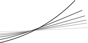
each subject to normalisation and shown in figure 3. Considering a filament with a curved centreline, corresponding to the initial condition of figure 4(a), with $N=100$ and $\epsilon =0.02$ we compute $\boldsymbol{\mathsf{A}}$ using both the RNS methodology and the inbuilt quadv routine in MATLAB®, with the numerical quadrature set to a tolerance of $10^{-12}$ and denoting the results of these computations by $\boldsymbol{\mathsf{A}}_{{RNS}}$ and $\boldsymbol{\mathsf{A}}_{{Q}}$, respectively. We write $\mathcal {E}$ for the relative matrix infinity norm error between these two results, defined explicitly as

(4.2)\begin{equation} \mathcal{E} = \frac{\left\lVert \boldsymbol{\mathsf{A}}_{{RNS}} - \boldsymbol{\mathsf{A}}_{{Q}}\right\rVert_{\infty}}{\left\lVert \boldsymbol{\mathsf{A}}_{{Q}}\right\rVert_{\infty}}. \end{equation}

These relative errors are shown in figure 3, each of which can be seen to be several orders of magnitude lower than the asymptotic slenderness parameter. The rapidly varying curvature of case (c) gives rise to the largest error, consistent with the restrictions imposed on the derivatives of $\chi$ in (3.29), with the derivatives of $\chi$ in case (c) being orders of magnitude greater than in cases (a) and (b). Computations were performed on modest hardware (Intel® Core$^{{\rm TM}}$ i7-6920HQ CPU), with the wall time for the RNS method being over two orders of magnitude less than that of the quadrature implementation, representing a significant improvement in computational efficiency for minimal reduction in accuracy. These observations of efficiency and accuracy hold for a range of considered body centrelines and radius functions, and are robust to variations in the slenderness parameter $\epsilon$.

Figure 3. Example radius functions and the relative error $\mathcal {E}$ of using the RNS method in constructing the operator $\boldsymbol{\mathsf{A}}$ compared with a quadrature rule of tolerance $10^{-12}$. In each of the three cases, we note a small matrix infinity norm error $\mathcal {E}$, largest in case (c) where curvature of the radius function is rapidly varying. Here we have considered a curved filament in a dimensionless framework with $N=100$ segments, having taken $\epsilon =0.02$ and radius functions corresponding to (4.1). The filament centreline corresponds to the initial condition of figure 4(a), and shapes are shown stretched vertically for visual clarity.

Figure 4. The relaxation of a symmetric filament, simulated with $N=40$ segments for $E_h=9600$. (a) Relaxation dynamics qualitatively matches that of Walker et al. (Reference Walker, Ishimoto, Gadêlha and Gaffney2019), in agreement with intuition and preserving the symmetry of the initial condition. (b) Distance translated by the centre of mass of the filament, as computed by the presented RNS methodology and the RSS approach of Walker et al. (Reference Walker, Ishimoto, Gadêlha and Gaffney2019), analytically zero and captured approximately here, having taken $N=40$ and $\epsilon =0.02$. Here, we have considered a filament with dimensionless shape $\eta (s')=\sqrt {1-s'^2}$, corresponding to a prolate ellipsoid, although note that this information is not captured by the typical slender-body ansatz, as implemented in Walker et al. (Reference Walker, Ishimoto, Gadêlha and Gaffney2019).

4.2. Invariants of free-filament motion

The coarse-grained framework for filament elasticity is similar to that presented and derived in the recent work of Walker et al. (Reference Walker, Ishimoto, Gadêlha and Gaffney2019), where it was extensively verified and benchmarked, utilising the stiff solver ode15s provided in MATLAB® with relative and absolute tolerances of $10^{-6}$ (Shampine & Reichelt Reference Shampine and Reichelt1997). However, due to the modification of considering a piecewise-constant discretisation of the force density $\boldsymbol {f}$, akin to the study of Moreau et al. (Reference Moreau, Giraldi and Gadêlha2018), we additionally verify the presented methodology in the case of a relaxing symmetric filament. Having taken $N=40$ and $\epsilon =0.02$, in figure 4 we showcase the simulated dynamics of an initially symmetric filament relaxing to a straight configuration, during which we see that symmetry is preserved. Owing to the filament having no net force or torque act upon it, the centre of mass should not deviate from its initial position. Computing the translation of the centre of mass over the motion, a quantitative measure of framework accuracy, in figure 4(b) we see that this approximate constancy is preserved numerically with errors of the order of $10^{-3}L$, improved by an order of magnitude when compared to the previous methodology of Walker et al. (Reference Walker, Ishimoto, Gadêlha and Gaffney2019).

4.3. Comparison against existing theories

We now more thoroughly compare and contrast the presented elastohydrodynamic framework against two existing approaches, in particular the published RSS methodology of Walker et al. (Reference Walker, Ishimoto, Gadêlha and Gaffney2019) and a resistive force theory (RFT) formulation based on that of Moreau et al. (Reference Moreau, Giraldi and Gadêlha2018). The latter RFT method is as described in the work of Walker et al. (Reference Walker, Ishimoto, Gadêlha and Gaffney2019), although we make use of the resistive coefficients of Hancock (Reference Hancock1953) and Gray & Hancock (Reference Gray and Hancock1955), with the normal resistive coefficient twice that of the tangential coefficient. A detailed comparison of the existing RFT and RSS hydrodynamic methodologies is presented in the work of Walker et al. (Reference Walker, Ishimoto, Gadêlha and Gaffney2019).

4.3.1. A relaxing filament

We simulate the free relaxation of a bent filament, with the $\theta _i$ initially equally spaced and increasing between $-{\rm \pi} /4$ and ${\rm \pi} /4$ to correspond to a filament of constant curvature, via each of the three methodologies, picking a common but arbitrary elastohydrodynamic number of $E_h=9600$ and setting $N=40$. The filament has aspect ratio 1 : 100, corresponding to $\epsilon =0.02$ in the RNS framework and $\epsilon =0.01$ in the RFT and RSS approaches. Simulating until a dimensional time of 100 s, at which point the RNS solution is nearing complete relaxation to a straight configuration, we display snapshots of the computed solutions and some associated metrics in figure 5. Immediately evident is a qualitative similarity between the computations, though there is some pairwise disagreement throughout the motion. Most prominent are differences in the time scale of relaxation, as can be seen in the maximum curvature plot of figure 5(b), with the RFT solution relaxing more slowly than the predictions by non-local theories. We more concretely quantify the overall differences between methodologies at a given time $t$ via the measure $D$, defined for a computed solution $\boldsymbol {x}(s,t)$ by

(4.3)\begin{equation} D(t)^2 = \frac{1}{L}\int\limits_0^L \left\|\boldsymbol{x}(s,t) - \boldsymbol{x}_{{RNS}}(s,t)\right\|_2^2\,\mathrm{d}s, \end{equation}

relative to the RNS solution $\boldsymbol {x}_{{RNS}}$. The evolution of this distance measure for the RFT and RSS approaches is shown in figure 5(c), and demonstrates that, whilst differences between solutions are indeed small, being on the scale of $\epsilon$ in this particular case, these distinctions persist throughout the motion.

Figure 5. Comparing methodologies via the relaxation of a symmetric filament, simulated with $N=40$ segments for $E_h=9600$. Each starting from an initial curved configuration, shown dotted in (a), we simulate the relaxation dynamics via RFT, RSS and RNS methodologies. (a) Shown at the same instant in time (30 s) are the filament configurations as computed by the three methodologies, with the filament shapes broadly similar although showing some minor differences. Only half of the filament is shown, appealing to the preserved symmetry, and the shared initial condition is shown as a dotted curve. (b) The maximum filament curvature as a function of time, highlighting greater distinctions between the methodologies. (c) The difference between filament configurations at time $t$, defined by $D^2 = \int \left\|\boldsymbol {x}_{{O}} - \boldsymbol {x}_{{RNS}}\right\| _2^2\,\mathrm {d}s/L$, quantifies the difference between the RNS method, denoted $\boldsymbol {x}_{{RNS}}$, and the results of the other frameworks, denoted $\boldsymbol {x}_{{O}}$. With a filament aspect ratio of 1 : 100 here, overall differences between computations appear only slight, with the exception of the longer time scale of the RFT solution compared to the non-local methodologies. In the RNS framework, we have considered a filament with dimensionless shape $\eta (s')=\sqrt {1-s'^2}$, corresponding to a prolate ellipsoid, although note that this information is not captured by the RFT or RSS frameworks.

With elastohydrodynamic simulations appearing broadly similar at the level of detail considered thus far, we also note a common computational efficiency of the frameworks, with even the more complex regularised non-uniform segments approach computing the relaxation dynamics in a number of seconds. Indeed, this is replicated throughout further testing for each of a wide array of initial conditions, and is robust to variations in the radius function $\eta (s')$ and the filament aspect ratio. Thus, despite employing a more sophisticated slender-body ansatz, we see retained in the RNS methodology the desirable efficiency associated with the existing coarse-grained frameworks.

4.3.2. A simple filament in flow

From the agreement seen above in the case of a relaxing filament, one might expect that the theoretical refinement offered by the RNS approach over the simpler and cruder RSS methodology is minimal in practice. However, more significant differences are indeed present.

We consider perhaps the most simple possible filament simulation: the dynamics of an initially straight filament in a uniform background flow, with a background flow $\boldsymbol {u}_b$ incorporated into the current framework via the mapping $\boldsymbol {u}\mapsto \boldsymbol {u}-\boldsymbol {u}_{b}$ as in the work of Walker et al. (Reference Walker, Ishimoto, Gadêlha and Gaffney2019). The simulated filament should exhibit trivial motion and deformation, merely translating with the background flow and retaining its straight configuration. Both the RNS and RSS methodologies successfully replicate this behaviour, and solution time is negligible. However, a noted issue of methods based on regularised Stokeslet segments and similar approaches are endpoint oscillations in the computed force density $\boldsymbol {f}$, present in each of the works of Cortez (Reference Cortez2018), Walker et al. (Reference Walker, Ishimoto, Gadêlha and Gaffney2019) and Hall-McNair et al. (Reference Hall-McNair, Montenegro-Johnson, Gadêlha, Smith and Gallagher2019), which persist even with mesh refinement.

Here, we explicitly compute the force density on a straight filament of aspect ratio 1 : 100 in a unit background flow $\boldsymbol {u}_b=\boldsymbol {e}_y$ using both the RNS and RSS approaches, where $\boldsymbol {e}_y$ is perpendicular to the filament tangent. In figure 6(a–c) we present the magnitude of the computed force density on the filament from $s=0$ to $s=L$ for various body radius functions, appealing to symmetry and noting that the force density is identically zero in the direction of the filament tangent. In each case, we observe the oscillations of the RSS force density near the endpoints of the slender body, with the RSS solution being fundamentally independent of the radius function, whilst the piecewise-constant RNS solution essentially eliminates these oscillations. We have taken $N=200$ in figure 6(c) in order to capture the highly oscillatory radius function of figure 3(c), consistent with the error analysis of § 3.3, taking $N=100$ in the other cases.

Figure 6. The computed force densities and errors in surface velocity for straight filaments in unit uniform flow, with shapes corresponding to figure 3. Here, we have used an aspect ratio of 1 : 100, corresponding to $\epsilon =0.02$ for the RNS methodology, and we recall that the slender-body theory upon which it is based is accurate to $O(\epsilon )$. In (a–c) we note the presence of significant oscillations near the ends of the filament for the RSS solution, absent from the RNS computation. (d–f) We report the error in the surface velocity for a unit magnitude background flow $\boldsymbol {u}_b=\boldsymbol {e}_y$, from which we note the significant improvement in accuracy afforded by the RNS methodology over the RSS approach. In particular, the RNS error is at least an order of magnitude less than the RSS error, except perhaps at the very endpoints of the filament, with the RSS methodology making little systematic attempt to satisfy the boundary condition on the surface. We have taken $N=100$ in (a,b,d,e), whilst in (c,f) we have taken $N=200$, with the highly curved radius function of figure 3(c) requiring reduced $\Delta \mathrm {s}$ to yield comparable accuracy to the other, simpler cases. (a,d), (b,e) and (c,f) correspond to the shapes shown in (a), (b) and (c) of figure 3.

Perhaps more pertinent, and indeed the motivation behind the use of the ansatz of Walker et al. (Reference Walker, Curtis, Ishimoto and Gaffney2020a), is the velocity boundary condition on the filament. We explicitly evaluate the flow velocity on the surface of the filament via both the RNS and RSS methods, sampling at 1000 uniformly spaced points on the surface, and show the infinity norm error in the computed velocity in figure 6(d–f) as a function of dimensionless shifted arclength $s'$. Notably, the RSS approach is consistently inaccurate along the length of the slender body, yielding approximately 5 % errors over the entire surface, corresponding to five times the regularisation parameter of the RSS method. The RNS methodology significantly improves upon this, with limitingly small error along the majority of each of the slender bodies in both figures 6(d) and 6(e), with errors of approximately $2\epsilon$ near the endpoints of the slender body in figure 6(e). In particular, these errors are of the same order as those found in the original evaluation of the slender-body theory by Walker et al. (Reference Walker, Curtis, Ishimoto and Gaffney2020a), with the impact of moving away from quadrature therefore minimal in all but figure 6(f), which is improved by reducing $\Delta \mathrm {s}$ to once again accommodate the oscillatory radius function. Thus, we observe that the use of the RNS methodology affords significant gains in the accuracy of the no-slip boundary condition over other approaches. Convergence of this velocity error as a function of $N$ and $\epsilon$ is illustrated in Appendix E for the case of figure 3(b).