


1 Introduction
Labor economics has long recognized the role of monetary incentives in determining workers’ effort (Lazear Reference Lazear2018). The effectiveness of monetary incentives that are tied to performance is well established. Behavioral economics added new insights to the effect of these conditional rewards by showing that their effectiveness is subject to psychological factors, such as crowding out of intrinsic motivation (Gneezy and Rustichini Reference Gneezy and Rustichini2000) and choking-under-pressure (Ariely et al. Reference Ariely, Gneezy, Loewenstein and Mazar2009; Hickman and Metz Reference Hickman and Metz2015).Footnote 1 This literature also discovered alternative incentive mechanisms, often inspired by studies in psychology, that can boost workers’ effort at no extra monetary cost. Among such mechanisms are goal-setting (Gómez-Miñambres Reference Gómez-Miñambres2012; Corgnet et al. Reference Corgnet, Gómez-Miñambres and Hernán-González2015, Reference Corgnet, Gómez-Miñambres and Hernán-González2018), performance ranking (Blanes i Vidal and Nossol Reference Blanes i Vidal and Nossol2011), and framing (Hossain and List Reference Hossain and List2012). A recent World Bank Report highlights behavioral mechanisms as an important incentive tool in developing countries (World Bank Group Reference Group2015).
Despite the convergence of economic and psychological insights on the determinants of effort, an important strand of psychological literature remains untapped by economists. A psychological theory of motivation called motivational intensity theory posits that the primary determinant of effort is task difficulty (Brehm and Self Reference Brehm and Self1989; Wright Reference Wright1996). Task difficulty can be defined as a characteristic of a task that, when increased, reduces the probability of success in the task for any given level of effort.Footnote 2 Task difficulty is conceptually different from the cost of effort, even though the two concepts are sometimes mixed in the literature (Bremzen et al. Reference Bremzen, Khokhlova, Suvorov and Van de Ven2015).Footnote 3 I attempt to close this gap by proposing a theoretical mechanism behind the effect of task difficulty on effort and by causally testing this mechanism in an incentivized experiment.
Motivational intensity theory assumes that effort investment in completing a task is determined by the motivation to avoid wasting energy. This implies that effort is determined by the minimum amount of work needed to complete a task, as long as success seems possible and beneficial (Wright Reference Wright1996; Brehm and Self Reference Brehm and Self1989).Footnote 4 The main prediction of the theory, which follows directly from its main assumption, is that effort increases with task difficulty up to a certain point. A further increase in difficulty causes effort to drop leading to an inverse-U pattern of effort response. Motivational intensity theory views monetary rewards as a mediating factor in effort provision that determines the point at which effort as a function of difficulty starts to drop.
Empirical studies in psychology provide extensive evidence for the inverse-U relationship between task difficulty and effort in the context of a direct effect of difficulty on effort (Smith et al. Reference Smith, Baldwin and Christensen1990; Richter et al. Reference Richter, Friedrich and Gendolla2008; Richter Reference Richter2015), as well as the effect of difficulty on effort interacted with other factors, such as learning and ability (Brouwer et al. Reference Brouwer, Hogervorst, Holewijn and van Erp2014; Latham et al. Reference Latham, Seijts and Crim2008), mood and fatigue (Brinkmann and Gendolla Reference Brinkmann and Gendolla2008; LaGory et al. Reference LaGory, Dearen, Tebo and Wright2011; Silvestrini and Gendolla Reference Silvestrini and Gendolla2009, Reference Silvestrini and Gendolla2011), motivation (Capa et al. Reference Capa, Audiffren and Ragot2008; Gendolla and Richter Reference Gendolla and Richter2005; Gendolla et al. Reference Gendolla, Richter and Silvia2008), and anticipated difficulty (Wright Reference Wright1984; Wright et al. Reference Wright, Contrada and Patane1986).Footnote 5 Task difficulty has also been proposed as an important factor in activating analytical reasoning (Alter et al. Reference Alter, Oppenheimer, Epley and Eyre2007) and achieving goals (Labroo and Kim Reference Labroo and Kim2009). The majority of these studies focus on physiological correlates of effort, such as cardiovascular activity, as originally suggested by Wright (Reference Wright1996). Subjects in these studies are given a task that can vary in difficulty, such as a memory task (Richter et al. Reference Richter, Friedrich and Gendolla2008). Effort is measured by the difference in the cardiovascular activity of subjects before and during performing a task. A common finding in this line of research is that subjects’ effort initially increases with task difficulty but then drops. This effect appears to be quite universal in that it is observed regardless of the nature of a task (cognitive, physical, or social).
A natural question arises of whether the inverse-U effect of difficulty on effort can be observed in an economic environment. Addressing this question is important for, at least, two reasons. First, understanding the role of difficulty and its interaction with other incentive elements, such as extrinsic monetary rewards, is relevant for principals who are seeking to design optimal incentive schemes for employees (Holmström Reference Holmström2017). Second, understanding the theoretical mechanisms behind the role of task difficulty in effort provision is relevant for researchers who are using models of effort provision to explain workers’ behavior in the labor market or to predict the potential effects of policy interventions.
I seek to accomplish two goals: first, to empirically study the effect of difficulty on effort and its interaction with monetary rewards; and second, to use this evidence to improve our understanding of the mechanisms behind effort provision and, in particular, to clarify the modeling assumptions that are needed to generate different patterns of effort response to difficulty.Footnote 6 In the empirical part, I set up an incentivized experiment that follows a chosen effort framework (Fehr et al. Reference Fehr, Gächter and Kirchsteiger1997; Abeler et al. Reference Abeler, Altmann, Kube and Wibral2010; Charness et al. Reference Charness, Cobo-Reyes, Jiménez, Lacomba and Lagos2012). Subjects assume the roles of agents who choose how much effort to exert in a series of projects. The probability of a project’s success depends on a subject’s chosen effort level and on a project’s difficulty. Higher difficulty reduces the probability of success on a project for any given level of effort. Monetary rewards consist of an unconditional (wage) and conditional (bonus) parts. The cost of effort is monetary and is subtracted from a project’s monetary outcome. I vary difficulty, monetary rewards, and cost within subjects and observe how this exogenous variation affects subjects’ effort levels. The chosen effort framework allows me to precisely define and observe difficulty and effort, and to derive sharp testable hypotheses.
To establish theoretical predictions, I use a very general model of effort choice under risk that allows for a utility function that is potentially non-separable in money and effort, as in Mirrlees (Reference Mirrlees1971). Allowing for such a general utility function is necessary, since, as I show in the comparative statics analysis, the pattern of complementarity between effort and money in the utility function, together with the pattern of complementarity between effort and difficulty in the probability of success function, determines the overall effect of difficulty on effort. I consider two alternative models of agents’ preferences. First, I use a benchmark Expected Utility (EU) model in which an agent chooses effort to maximize the weighted average of outcomes’ utilities with the weights being the probabilities of each outcome. I show, in particular, that in the present experimental design a risk-averse agent would monotonically decrease her effort in response to higher difficulty. Interestingly, a model with an additively separable cost of effort, which is a workhorse model in the literature, predicts that higher difficulty would lead to no change in effort at all.
Given that the inverse-U relationship between effort and difficulty in the present experiment cannot be generated by the standard EU-approach, I consider an alternative model that can deliver such a relationship. The alternative model allows for probability weighting, as in the Cumulative Prospect Theory (CPT) (Tversky and Kahneman Reference Tversky and Kahneman1992). In this model, the agent also chooses effort to maximize a weighted average of outcomes’ utilities, but now the weights are the probabilities that are transformed using a probability weighting function. I show that allowing for the probability weighting makes it possible to generate richer predictions about the potential effect of difficulty on effort. In particular, if the probability weighting function is inverse-S-shaped (respectively, S-shaped), the pattern of effort response to difficulty in the present experiment would be U-shaped (respectively, inverse-U-shaped). I argue that probability weighting is the only plausible channel that can generate a non-monotonic effect of difficulty on effort.
I find that monetary rewards affect effort in the predicted direction. Conditional rewards, on average, have a strong positive effect on effort, while the effect of unconditional rewards is positive but weak. These results are consistent with the previous findings in the literature (Gneezy and List Reference Gneezy and List2006; DellaVigna and Pope Reference DellaVigna and Pope2018). Despite strong statistical significance, the economic significance of conditional rewards is somewhat disappointing: doubling the conditional rewards increases effort only by 20%. Making the cost of effort steeper leads to a sharp decrease in effort, as predicted. This result is consistent with the findings in the contest literature (Dechenaux et al. Reference Dechenaux, Kovenock and Sheremeta2015), as well as in the studies employing real-effort tasks (Goerg et al. Reference Goerg, Kube and Radbruch2019).
I find that the effect of difficulty on effort is inverse-U-shaped, which supports the hypothesis of an S-shaped probability weighting. This result is new to the economics literature.Footnote 7 It does echo, however, the findings from the studies on the motivational intensity theory. Interestingly, the magnitude of the effect of difficulty is on par with the magnitudes of the effects of conditional rewards or costs. I find that difficulty mediates the effects of monetary rewards. Conditional rewards are most effective at the intermediate and high levels of difficulty. The inverse-U effect of difficulty on effort refutes the benchmark EU-based model of effort and supports the alternative model with an S-shaped probability weighting. I further confirm this in a structural analysis by estimating the parameters of the probability weighting function. While a typical finding in the literature on risk preferences is an inverse-S-shaped probability weighting (Wu and Gonzalez Reference Wu and Gonzalez1996; Bruhin et al. Reference Bruhin, Fehr-Duda and Epper2010; l’Haridon and Vieider Reference l’Haridon and Vieider2019), the subjects in the DellaVigna and Pope (Reference DellaVigna and Pope2018) study also tended to underweight small probabilities (implied by an S-shaped weighting) in a real-effort experiment.Footnote 8
The present findings have several important implications for the design of incentive schemes and modeling effort. The strong incentive effect of task difficulty suggests that managers should take this effect into account when assigning tasks to their subordinates. A manager can expect that it will take workers more effort to complete a moderately hard task than an easy task. However, workers might not devote as much effort to a very hard task as the manager would desire. This behavioral response to high difficulty can substantially lower a worker’s performance by amplifying the direct negative effect of difficulty on performance. A manager, however, can counter this detrimental behavioral effect of difficulty using conditional rewards, since they are most effective when difficulty is high.
From a theoretical perspective, the workhorse model with an additively separable cost of effort might not be a good behavioral assumption in some cases. My results suggest that supplementing the workhorse model with probability weighting can better explain certain patterns of effort provision and yield higher predictive power. The implications of probability weighting on effort provision in other contexts, thus, deserve further investigation.
The uncovered effect of difficulty on effort has general methodological implications for using the existing effort tasks and designing new ones (Gill and Prowse Reference Gill and Prowse2012; Gächter et al. Reference Gächter, Huang and Sefton2016). Experimental designs should control for task difficulty since it can have a strong and non-monotonic effect on subjects’ effort. The interaction effect between task difficulty and incentives can be exploited to ensure that monetary incentive treatments do not suffer from a “ceiling-effect” problem. Setting task difficulty to an intermediate level should provide enough room for monetary incentives to affect subjects’ effort.
I proceed as follows. Section 2 discusses the related literature. Section 3 describes the experimental procedures, design, and treatments. Section 4 presents the theoretical framework and derives testable hypothesis. Section 5 discusses the results of the experiment and estimates a structural model motivated by the observed behavioral patterns. Section 6 concludes.
2 Related literature
Most closely related to my design is the research by Vandegrift and Brown (Reference Vandegrift and Brown2003) that studies the interactive effect of task difficulty and conditional monetary rewards on performance in a tournament environment. It finds that monetary rewards do not have any effect on performance for easy tasks, but do have a positive effect for difficult tasks.Footnote 9 My results confirm the existence of the interaction effect between task difficulty and conditional rewards, while simultaneously extending them by presenting new evidence on the direct effect of task difficulty on effort. An additional contribution of my work is that it proposes and tests a novel theoretical mechanism behind the observed behavior.
Closely related to the effect of task difficulty on effort and its interaction with conditional rewards is the literature on goal-setting. Corgnet et al. (Reference Corgnet, Gómez-Miñambres and Hernán-González2015) conduct a laboratory principal-agent experiment and find that principals tend to set challenging but attainable performance goals for agents, which increases agents’ performance relative to a no-goals baseline. They also report that the effect of goal-setting on effort is stronger under high monetary rewards. Smithers (Reference Smithers2015) conducts a laboratory experiment and finds that setting exogenous goals in an addition task increases subjects’ performance, with the effect being most pronounced in the male participants. Goerg and Kube (Reference Goerg and Kube2012) conduct a field experiment at a campus library in which subjects were paid to sort books. They report that both exogenous and endogenous goal-setting leads to higher performance. These results are similar to the present findings, however, goal difficulty and task difficulty are not equivalent (Campbell and Ilgen Reference Campbell and Ilgen1976). Apart from having a difficulty component, goals also have a reference point component (Heath et al. Reference Heath, Larrick and Wu1999).
Going beyond the individual decision-making setting, the question of what drives effort levels takes a central place in the contest literature. This literature, however, does not explicitly consider the difficulty of winning a contest. One can interpret the number of players in a contest as a variable that is positively related to the difficulty of winning a prize. Such an interpretation is possible since increasing the number of players decreases the probability of winning a prize, all else equal, which is consistent with the definition of difficulty assumed in the present paper. While the theoretical relationship between the number of players and effort is ambiguous, experiments typically find a decreasing relationship (Dechenaux et al. Reference Dechenaux, Kovenock and Sheremeta2015).
The analysis of the effects of conditional and unconditional rewards in the present work is related to the literature on the behavioral effects of monetary rewards. Hossain and List (Reference Hossain and List2012) conduct a field experiment at a Chinese manufacturing firm. They randomly assign workers to one of two conditions: in one condition, workers are paid a bonus upon reaching a given performance goal; and in the other condition, workers are paid a bonus in advance and lose it if they do not reach a performance goal. Consistent with the loss aversion hypothesis, the workers’ performance was higher in the second condition. Gneezy and List (Reference Gneezy and List2006) conduct a field experiment at a campus library in which they vary the unconditional rewards paid to their subjects for arranging books. They find that increasing rewards has a positive but short-lived effect on the subjects’ effort. A similar finding is reported by Jayaraman et al. (Reference Jayaraman, Ray and de Vèricourt2016) who study the effort response of tea pluckers in India to an increase in their unconditional rewards caused by a change in contracts. Hennig-Schmidt et al. (Reference Hennig-Schmidt, Sadrieh and Rockenbach2010) show that the positive effect of unconditional rewards occurs only when workers understand the benefit of their work to the principal, which triggers positive reciprocity. The weakly positive effect of unconditional rewards reported in the present paper is consistent with their findings.
Apart from the literature in economics, the present work is inspired by, and thus related to, the literature in psychology on motivational intensity theory (Brehm and Self Reference Brehm and Self1989; Wright Reference Wright1996). The present paper clarifies the link between task difficulty and effort from the perspective of economic theory and confirms the existence of an inverse-U relationship in an economic environment. Richter et al. (Reference Richter, Friedrich and Gendolla2008) use a laboratory experiment in which students participated in several rounds of a memory task (Sternberg Reference Sternberg1966). The difficulty of the task was manipulated by the time during which the sequence of letters to be memorized appeared on the screen. Subjects’ cardiovascular activity was evaluated right before and during the task, and the difference was used as a measure of effort. The study finds that effort increases up to the “high” level of difficulty and drops sharply at the “impossible” level. Smith et al. (Reference Smith, Baldwin and Christensen1990) use a different task in which subjects had to give a convincing speech to an audience. The difficulty of the task depended on how convincing the speech should have been. The study measured effort using cardiovascular activity before and during the task. Effort due to anticipated difficulty (measured just before the performance) followed the same inverse-U pattern as effort during the performance. The inverse-U pattern of effort due to anticipated difficulty is also reported by Wright et al. (Reference Wright, Contrada and Patane1986). The subjects in the study did not actually perform a task, but rather were given task instructions (a variation on the memory task) along with an explicit statement about its difficulty after which the cardiovascular measurements were taken. The inverse-U pattern of efforts in response to difficulty is found in the survey data, as well. Brockner et al. (Reference Brockner, Grover, Reed and Dewitt1992) study how work effort is related to job insecurity (which can be interpreted as the difficulty of staying on a job) in the survey of workers in a nation-wide store chain and find that effort is highest at the intermediate level of job insecurity.
3 Experimental design
3.1 Procedures
The experiment was conducted at the ExCEN lab at Georgia State University (GSU) in May–June 2015. A total of 98 subjects participated in the experiment over the course of six sessions. The subjects were recruited using an automated system that randomly invited participants from a pool of more than 2000 students who signed up to participate in economic experiments. The subjects in the study were undergraduate students at GSU invited to participate via email. Each session was run on computers and lasted for roughly 1.5 h. The subjects received a show-up fee of $5 and the payoffs from decisions tasks.Footnote 10 The average payment per subject was $45.89 (the minimum payment was $5, and the maximum was $100), including the show-up fee.
Table 1 summarizes the demographic characteristics of the sample. The sample had equal shares of males and females. The racial composition was dominated by African American students: they accounted for 62% of the sample, while Caucasian students represented 14% of the sample. An average student’s age was slightly above 21 years. The majority of subjects were in the advanced stages of a college program: more than half of participants were either juniors or seniors. Only 10% of the subjects came from an Economics or Finance major, which alleviates the concern that the observed behavior could be driven by the subjects sophisticated in economics.
Table 1 Socio-demographic characteristics of the sample

|
Characteristic |
Mean |
|---|---|
|
Gender |
|
|
Male |
0.48 |
|
Female |
0.48 |
|
Other/prefer not to answer |
0.04 |
|
Race and age |
|
|
Black or African American |
0.62 |
|
Asian |
0.18 |
|
White or Caucasian |
0.14 |
|
Other/prefer not to answer |
0.05 |
|
Age |
21.29 |
|
Year in program and major |
|
|
Freshman |
0.04 |
|
Sophomore |
0.18 |
|
Junior |
0.24 |
|
Senior |
0.45 |
|
Graduate |
0.05 |
|
Prefer not to answer |
0.03 |
|
Econ or finance major |
0.10 |
3.2 Effort task
In each round of the effort task, a subject was given a project that had two possible outcomes: success or failure.Footnote 11 A project was presented to subjects graphically, with outcomes and probabilities shown both in numerical format and as colored bars. The left part of the screen showed the monetary outcomes (revenue, cost, and profit) in the case of success, while the right part of the screen showed the monetary outcomes in the case of failure. The probabilities corresponding to each outcome were displayed below the monetary outcomes. At the bottom of the screen was a slider which subjects could use to input their effort level.
Each project was characterized by four treatment variables that varied across rounds for each subject. These variables are: bonus (z), wage (w), difficulty (
 ), and cost (k). In the case of success, a project yielded a high revenue (the sum of a wage and a bonus), and in the case of failure it yielded a low revenue (a wage only). Wage represents an unconditional (on performance) reward and bonus represents a conditional reward. The difficulty of a project affected the probability of success. Higher difficulty resulted in a lower probability of success for any given level of effort. The cost variable affected the steepness of the cost-of-effort function. The experiment was presented to subjects in a meaningful labor context with terms such as “revenue,” “effort,” and “difficulty.”Footnote 12 While it is possible that the meaningful context can have a framing effect, I believe that the benefits of using context in the present experiment outweigh potential costs. First, context enhances subjects’ understanding of an arguably complex decision-making task (Alekseev et al. Reference Alekseev, Charness and Gneezy2017; Hsiao et al. Reference Hsiao, Kemp and Servátka2019). And second, the labor context is appropriate given that the present study seeks to contribute to the understanding of effort provision.
Subjects could choose any integer effort level a between 0 and 100 percent. The chosen level of effort had a twofold effect: on the probability of success, and on a project’s profit (revenue minus cost). Higher effort increased the probability of success but led to lower profits. The subjects incurred the cost of effort regardless of the outcome of a project. When deciding what effort level to choose, the subjects therefore faced a trade-off between a higher chance of the project being successful and lower profits. By moving the effort slider, subjects could clearly observe how a given effort level translates into monetary outcomes and probabilities for each outcome.
The use of the chosen, rather than real, effort framework is common in tournament (Bull et al. Reference Bull, Schotter and Weigelt1987) and principal-agent experiments (Fehr et al. Reference Fehr, Gächter and Kirchsteiger1997; Abeler et al. Reference Abeler, Altmann, Kube and Wibral2010; Charness et al. Reference Charness, Cobo-Reyes, Jiménez, Lacomba and Lagos2012). The primary motivation for this design is to allow for a clean test of theoretical predictions. Brüggen and Strobel (Reference Brüggen and Strobel2007) demonstrate that the chosen effort framework yields qualitatively similar results to the real effort framework in their setting, while allowing for a greater control.
The probability of success p as a function of effort a and difficulty
 was computed as

so that, effectively, the probability of success was a simple average between an effort level and a project’s ease,
 .Footnote 13 The cost of effort was computed as the square of effort multiplied by the cost variable k:

to induce a convex cost schedule. The subjects were informed of the linear relationship between the probability of success and effort and of the convex relationship between the costs and effort.
Subjects received feedback on the outcome of a project in every round.Footnote 14 The feedback was provided to ensure that subjects had a good understanding of the task, since quick feedback is crucial for learning and improving performance (Balzer et al. Reference Balzer, Doherty and O’Connor1989; Hoch and Loewenstein Reference Hoch and Loewenstein1989). This was justified by the complexity of the decision task, which had many alternatives to choose from (specifically, 101 levels of effort) and several decision-relevant variables to consider. After the outcome of a project was determined, the subjects could review the results of the current round on a summary screen.
Each subject played between 15 and 19 rounds of the effort task, which were preceded by five practice rounds.Footnote 15 After completing all the rounds, the payoff for the effort task was determined by randomly selecting one round. While paying randomly for one round is theoretically not incentive compatible with non-EU models (Harrison and Swarthout Reference Harrison and Swarthout2014; Cox et al. Reference Cox, Sadiraj and Schmidt2015), the provision of feedback after each round (i.e., playing out choices sequentially but paying for one choice randomly in the end) might alleviate this concern in practice (though not in theory), as suggested by Cox et al. (Reference Cox, Sadiraj and Schmidt2015). They show that estimated risk preferences are not significantly different between a treatment in which subjects made, and were paid for, only one choice (theoretically incentive compatible with any model) and a treatment in which subjects made multiple choices with feedback and were paid for a random round.
The four project characteristics (difficulty, wage, bonus, and cost) changed randomly across rounds, and subjects were aware of this. Each distinct combination of the values of these treatment variables represents a treatment. The three monetary treatment variables (w, z, and k) assumed one of the two possible values. Wage w assumed the values of 1 or 2, bonus z assumed the values of 2 or 4, and cost k assumed the values of 1 or 2. These values were multiplied by $10 and then presented to subjects. For instance, a treatment with
 and
and
 corresponded to a project with a low revenue of $10 and a high revenue of $30 = $10 + $20. Similarly, given an effort level of 40% and a treatment with
 , the cost of effort would be $3.2 = $20
 0.4
0.4
 . Difficulty assumed five values: 0, 0.25, 0.5, 0.75, and 1, which was important for identifying a potentially non-monotonic effect on effort.Footnote 16 The treatments were constructed from the permutations of the values of the treatment variables. The order of treatments was randomized on the subject level. Each subject made an effort choice in a given treatment only once.Footnote 17 Appendix A provides the summary of the treatments used in the experiment.
The within-subject design was chosen for three main reasons. First, the large number of treatments made it impractical to use a between-subject design. Second, the within-subject design allows for a deeper analysis of the subjects’ data and improves statistical power. Third, even though it is possible that subjects experience the experimenter demand effect by observing all the treatments (Charness et al. Reference Charness, Gneezy and Kuhn2012), it was unlikely in the present experiment. A relatively large number of treatment variables changing randomly between the rounds would make it extremely hard for subjects to infer patterns and the expected responses.
4 Theoretical framework
4.1 Environment
Consider an agent who works on a project with a stochastic binary outcome, success or failure. The project yields a wage
 regardless of the outcome and a bonus
 in the case of success. This is a standard setting in the principal-agent literature (Laffont and Martimort Reference Laffont and Martimort2009) The novel assumption is that the probability of success in the project is determined, in addition to the agent’s effort
 , by the project’s difficulty
 . The vector of the values of the project’s characteristics is denoted as
 .
.
Let X be a Bernoulli random variable encoding the project’s outcome. The agent’s revenue from the project is
 . The probability of success
 is a function of effort a and difficulty
 . I assume that p is twice continuously differentiable, increasing and concave in effort, and decreasing in difficulty.
If the cdf of X conditional on effort and difficulty is
 and pmf is
 (for
(for
 , and 0 otherwise), then for
 we have
 . This implies that the agent has an incentive to exert more effort, since the project endowed with a high effort level first-order stochastically dominates the project with a low effort level. However, there is a trade–off in that more effort leads to higher disutility from exerting it.
4.2 Preferences
I assume that the agent has preferences over money y and effort a represented by a utility function
 . The u function is assumed to have the standard properties: it is twice continuously differentiable, strictly increasing and concave in money, and is strictly decreasing and concave in effort, i.e., the marginal disutility of effort increases. I use a very general utility function that is potentially non-separable in money and effort, as in Mirrlees (Reference Mirrlees1971), as opposed to a more commonly used additively separable function (Abeler et al. Reference Abeler, Falk, Goette and Huffman2011; Hossain and List Reference Hossain and List2012; Jayaraman et al. Reference Jayaraman, Ray and de Vèricourt2016; DellaVigna and Pope Reference DellaVigna and Pope2018). The reason for this choice is that the additively separable specification turns out to be very restrictive in terms of the comparative statics effect of difficulty on effort.
Given that the agent exerts effort in a risky environment, I consider two alternative models of the agent’s preferences and show that the assumptions about these preferences play a crucial role in determining the effect of difficulty on effort. The first natural assumption is the EU model.
Assumption 1.A
(EU) The agent’s risk preferences are characterized as
I also explore an alternative model that allows for non-linear probability weighting, as in the CPT (Tversky and Kahneman Reference Tversky and Kahneman1992) or the Rank-Dependent Utility model (Quiggin Reference Quiggin1982). Probability weighting turns out to be critical for producing the non-monotonic effect of difficulty on effort.
Assumption 1.B
(PW) The agent’s risk preferences are characterized as

where
 is the decision weight of an outcome x, and
 is the success probability weighted by the probability weighting function
 , twice continuously differentiable and strictly increasing with
 and
and
 .
.
4.3 Optimal effort
Under Assumption Footnote 1.A the agent chooses the optimal effort level
 given the parameters of the problem
 by maximizing
 . If
. If
 , then the first-order necessary condition must hold:Footnote 18
Equation (3) means that in the optimum the marginal benefit from exerting more effort on the left-hand side must be balanced by the marginal cost of effort on the right-hand side. The marginal benefit represents the expectation of the utility weighted by
 , since the gain comes from the increased probability of success. It can be rewritten as
 , where
 is the utility gain between the success and failure given effort a. Written in this form, the marginal benefit is the marginal increase in the probability of success multiplied by the utility gain. The marginal cost is the expected marginal disutility of effort. It can be rewritten using the Mean Value Theorem as
 , where the cross-partial is evaluated at some point
 . This form will be useful for understanding the comparative statics of the model.Footnote 19 All the above results also hold under Assumption Footnote 1.B after replacing U,
 , f and p with
 ,
,
 ,
,
 and
and
 , respectively.
4.4 Special cases
Several special cases of the utility function u permit closed-form solutions. The first case is a separable utility function,
 , which is a popular specification in the literature. In this specification the utility of money v is linearly separable from the cost of effort c. Assume that
 is twice continuously differentiable, increasing and concave. With a quadratic cost of effort as in (2) and a linear probability of success as in (1), the optimal effort is
A notable feature of this specification is that the optimal effort does not depend on the project’s difficulty. As will be shown shortly, this is the consequence of the linearity of p and the additive separability of u, under which the cross-partial derivatives of both functions are zero. The optimal effort increases with the bonus and decreases with the cost k, which is intuitive. The increase in the wage causes the optimal effort to go down if v is strictly concave. This makes sense since if the agent can guarantee herself good result regardless of the outcome she will not have a strong incentive to exert effort. However, if v is linear, the optimal effort does not depend on wage and assumes a particularly simple form: z/(4k) .
The second case is a non-additively separable specification in which effort has a monetary cost to the agent, just like in the current experimental design, and the utility of money is exponential,
 , with
 being the constant absolute risk aversion (CARA) parameter. The benefit of using the exponential (CARA) utility is its analytical tractability. Assume that the cost of effort is quadratic and the probability of success is linear. It can be shown that in this case the optimal effort is given by
and the effect of difficulty on the optimal effort is negative because of the positive risk aversion parameter. Unlike in the additively separable case, u has a positive cross-partial derivative, which drives this result. It is worth noting that the optimal effort will not depend on the wage. As in the previous case, the optimal effort will increase with the bonus and decrease with the cost.
4.5 Comparative statics, difficulty
Under Assumption Footnote 1.A, the effect of the project’s difficulty on the optimal effort is given by
where
 are some numbers on
 . The sign of the effect crucially depends on the signs of the cross-partial derivatives of both u and p. This effect can be concisely stated as follows.
Proposition 1.A
If
 , then
 .
.
Assuming that
 , the effect of difficulty will have the same sign as this cross-partial derivative. Intuitively, this implies that if effort and difficulty are complements in the probability function, it is optimal to increase effort in response to a higher difficulty. Since higher difficulty reduces the probability of success, the optimal response is to compensate this reduction. On the other hand, if effort and difficulty are substitutes in p, it is optimal to reduce effort, which makes the reduction in the probability of success even higher.
Using Assumption Footnote 1.B instead, the formula in (5) remains valid after the appropriate change of non-tilde characters to tilde characters. Expanding, one obtains

where
 and
and
 are evaluated at
 . Note that if
 we are back to the EU case, since there would be no probability weighting. The sign of the effect of difficulty on effort now depends, in addition to the signs of the cross-partial derivatives of u and p, on the sign of
 . Assuming that
 , the effect of difficulty in this case can be concisely stated as follows.
Proposition 1.B
If
 and
and
 , then
 .
.
This result has an intuitive interpretation. If the agent exhibits probability pessimism,
 , she will reduce effort in response to a higher difficulty, as if she does not believe in her ability to affect the chances of success strong enough to accept the challenge. On the other hand, if the agent exhibits probability optimism,
 , she will raise effort in response to a higher difficulty.
The results obtained so far predict only a monotonic effect of difficulty on effort. The findings in psychology (Gendolla et al. Reference Gendolla, Wright, Richter and Ryan2012, Reference Gendolla, Richter and Silvia2008), however, suggest the existence of a non-monotonic inverse-U pattern. The question is what features of the model can produce such a non-monotonic effect. An inspection of the comparative statics formulas (5) and (6) reveals that in order to achieve a non-monotonic effect, the terms containing
 need to change their sign as
 changes. The only term that naturally has this feature is
 since experiments often find an inverse-S shape of the probability weighting function (Wu and Gonzalez Reference Wu and Gonzalez1996; Bruhin et al. Reference Bruhin, Fehr-Duda and Epper2010), which is concave for low values of p and convex for high values of p.
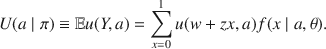
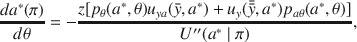
Assume for simplicity that both cross-partial derivatives or u and p are zero and that
 is inverse-S-shaped. The sign of the effect of difficulty then would change from positive, for small p, to negative, for high p. The difficulty is inversely related to p, hence one could expect that effort would increase (decrease) for high (low) values of difficulty, which implies a U-shaped pattern. Figure 1b illustrates this point by plotting the optimal effort as a function of difficulty for three different shapes of
 . In the simulation, I use the monetary cost of effort specification with the CRRA utility of money
 with
with
 and the one-parameter Prelec (Reference Prelec1998) weighting function
 . The cost and probability of success functions are specified as before. The optimal effort as a function of difficulty is U-shaped for an inverse-S-shaped probability weighting function and is inverse-U-shaped for an S-shaped probability weighting function. When there is no weighting, the optimal effort monotonically declines in difficulty as predicted by Proposition Footnote 1.A, since
 in this specification.
Fig. 1 Comparative statics under probability weighting
4.6 Comparative statics, bonus and wage
The effect of bonus on optimal effort is given by
which leads to the following result:
Proposition 2
If
 , optimal effort will increase with bonus.
This prediction makes sense intuitively, as a higher bonus means a better outcome in case of success, which in turn justifies higher effort. Both additively separable and exponential utility cases are examples of this result. Proposition Footnote 2 clarifies, however, that this result holds unambiguously only when money and effort are complements in the utility function.
The effect of wage on optimal effort is given by
which leads to the following result:
Proposition 3
If
 , optimal effort will decrease with wage.
This means that if the agent can guarantee herself higher revenue regardless of the outcome, she has an incentive to exert low effort, provided that u is submodular. This is true, for example, in the additively separable case.
Propositions Footnote 2 and Footnote 3 will still hold under the probability weighting assumption, since
 and
and
 have the same signs as p and
 , respectively.
4.7 Testable hypotheses
In the experiment, the probability of success function in (1) is linear and therefore
 . Moreover, the use of the chosen effort framework allows me to determine the sign of the cross-partial
 unambiguously. Since effort has a monetary cost to the agent, the utility function becomes
 , where
 is the utility of money, assumed to be twice continuously differentiable, increasing and concave, and
 is the cost of effort function given by (2), twice continuously differentiable, increasing and convex. Then the cross-partial of the utility function is
 , which implies that
 .
.
The analysis of the comparative statics shows that the effect of difficulty cannot be signed unambiguously, as different preference assumptions (EU, inverse-S-shaped probability weighting, or S-shaped probability weighting) yield competing predictions. The use of the chosen effort framework does allow me to sign the predicted effect of difficulty within a given preference assumption, hence the data will ultimately determine the winning assumption. Below I summarize the competing hypothesis derived so far.Footnote 20
Hypothesis 1.A
(Difficulty, decreasing) Subjects’ average effort will monotonically decrease with the project’s difficulty.
Hypothesis 1.B
(Difficulty, U-shape) Subjects’ average effort will first decrease, reach a minimum, and then increase with the project’s difficulty.
Hypothesis 1.C
(Difficulty, inverse-U-shape) Subjects’ average effort will first increase, reach a maximum, and then decrease with the project’s difficulty.
Turning to the effect of incentives, in the experiment u is supermodular and Proposition Footnote 2 applies directly leading to the following hypothesis:
Hypothesis 2
(Bonus) Subjects’ average effort will increase with the project’s bonus.
In the experiment,
 and therefore Proposition Footnote 3 cannot be applied to sign the effect of wage. We have seen that in the special case of exponential utility the optimal effort level did not depend on the wage. In the numerical simulations with CRRA utility, effort monotonically increases with wage. It is, therefore, reasonable to expect the following behavior.
Hypothesis 3
(Wage) Subjects’ average effort will monotonically increase with the project’s wage.
The experimental design includes one more treatment variable, k, which is the scaling factor of the cost of effort function. The comparative statics for the cost variable cannot be derived in a general model, since k only arises in the parametrizations of the model. The effect of k on the optimal effort, however, can be evaluated in the special cases we considered earlier. These special cases suggest the following behavior.
Hypothesis 4
(Cost of effort) Subjects’ average effort will decrease with the cost of effort.
5 Results
I begin by presenting the treatment effects of the monetary treatment variables and difficulty.Footnote 21 Then I show how the treatment effects of the monetary variables change conditional on the value of difficulty. The analysis concludes with the structural estimation of the model.
5.1 Treatment effects
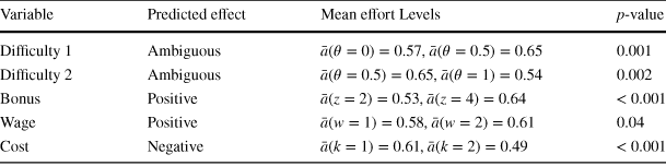
Table 2 shows the summary of the treatment effects. Figure 2 shows the empirical CDFs of subjects’ effort levels for different values of the treatment variables.Footnote 22 Since the dataset has a panel structure (every subject experiences multiple treatments), I first compute the mean effort levels for each value of a treatment variable for each subject and then report statistics for these subject-level means. To analyze the effect of wage, I use the subset of observations with
 . For the full sample, wage and cost are highly correlated, which is due to the nature of the design. In the experiment, cost cannot exceed wage, otherwise a negative profit could occur and subjects could lose money. When analyzing the effect of cost, the sample is restricted to observations in which
 for the same reason.
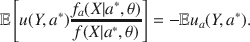
Figure 3 summarizes the treatment effects results by plotting the average treatment effects (ATEs) for all the treatment variables. An ATE for a variable is calculated as the change in the mean effort level (shown in Table 2) when the variable increases. The effect of difficulty is broken down into the first increase from 0 to 0.5 (Difficulty 1) and the second increase from 0.5 to 1 (Difficulty 2). The treatment variables are sorted by the magnitude of the ATE, which makes it easy to compare the effectiveness of different variables in affecting effort.
Table 2 Summary of treatment effects
|
Variable |
Predicted effect |
Mean effort Levels |
p-value |
|---|---|---|---|
|
Difficulty 1 |
Ambiguous |
|
0.001 |
|
Difficulty 2 |
Ambiguous |
|
0.002 |
|
Bonus |
Positive |
|
|
|
Wage |
Positive |
|
0.04 |
|
Cost |
Negative |
|
|


Difficulty 1 refers to the change in difficulty from 0 to 0.5. Difficulty 2 refers to the change in difficulty from 0.5 to 1. The p-values are from a Wilcoxon signed rank test (two-sided)
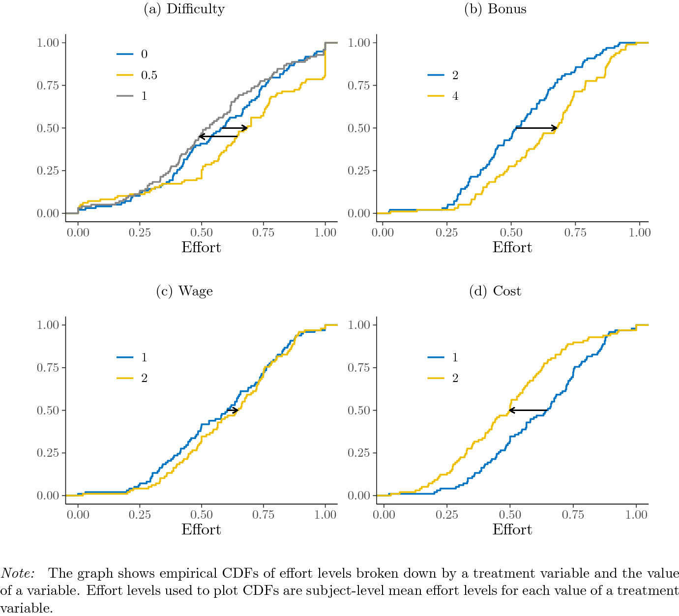
Fig. 2 Empirical CDFs of effort by treatment variable
The inverse-U effect of difficulty picks Hypothesis Footnote 1.C as the winning hypothesis and is new to the economics literature. The intuition behind this result is the following. When the probability weighting function is S-shaped, high difficulty corresponds to the case of low probability of success where the probability weighting function is convex (probability pessimism) and hence higher difficulty leads to lower effort. On the other hand, low difficulty corresponds to the case of high probability of success where the probability weighting function is concave (probability optimism) and hence higher difficulty leads to higher effort. This result, however, is consistent with the previous findings in psychology on the motivational intensity theory, as reviewed by Gendolla et al. (Reference Gendolla, Wright, Richter and Ryan2012). This literature finds that subjects increase their effort in response to higher difficulty up to a certain point after which effort is decreased. A remarkable feature of the present result is that changing difficulty produces a powerful incentive effect that is comparable to the effect of doubling the conditional reward or doubling the cost of effort, see Fig. 3. The effect of difficulty on effort, however, is more noisy than the effects of monetary rewards or cost.
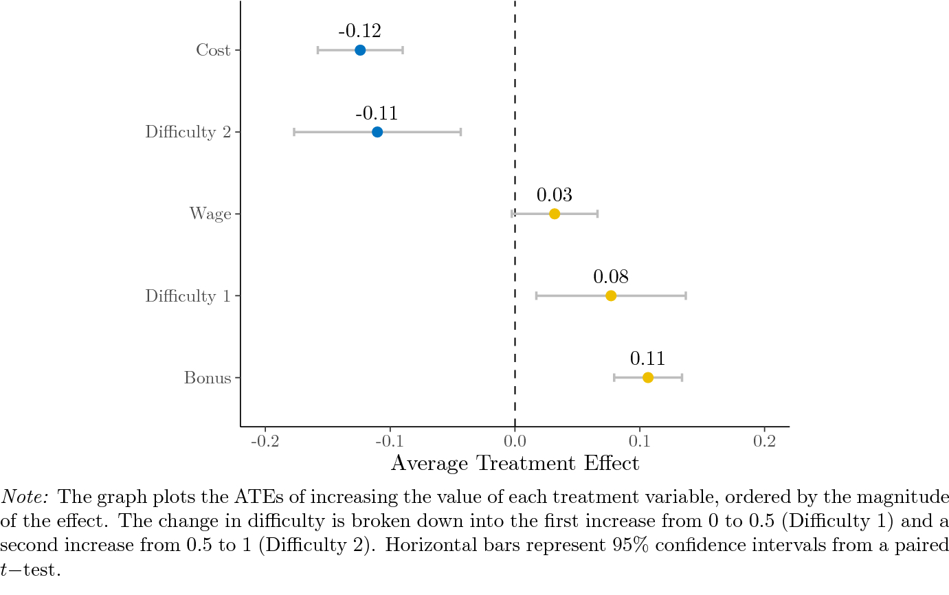
Fig. 3 Comparison of ATEs
Result 1
Subjects’ average effort first increases, reaches a maximum, and then decreases with the project’s difficulty.
The effects of conditional and unconditional rewards are consistent with the previous findings in the literature. The positive effect of a higher bonus supports Hypothesis Footnote 2 and is in line with the results reported in Lazear (Reference Lazear2000) and Hossain and List (Reference Hossain and List2012) and more recently by DellaVigna and Pope (Reference DellaVigna and Pope2018) and de Quidt et al. (Reference de Quidt, Haushofer and Roth2018). Some papers suggest that when conditional rewards are too small or too high, they can backfire and lead to lower effort either through crowding out of intrinsic motivation or choking-under-pressure (Gneezy et al. Reference Gneezy, Meier and Rey-Biel2011). I do not observe these negative effects in my data because the chosen effort framework leaves little space for these two channels and also because the level of conditional rewards in the experiment apparently did not hit either extreme. I do note, however, that while the effect of bonus is highly statistically significant, its economic significance is somewhat disappointing. Recall that in the experiment the monetary value of a bonus doubles from $20 to $40. This substantial change in stakes, however, does not lead to doubling effort, as a simple risk-neutral model (4) would suggest. Effort increases only by
 or by 0.52 standard deviations.
Result 2
Subjects’ average effort increases with the project’s bonus.
The weakly positive effect of higher wage supports Hypothesis Footnote 3 and is also consistent with the previous studies on the effect of unconditional rewards. A common finding is that unconditional rewards are effective in the short-run (Gneezy and List Reference Gneezy and List2006; Jayaraman et al. Reference Jayaraman, Ray and de Vèricourt2016) and when the reciprocity channel exists (Cohn et al. Reference Cohn, Fehr and Goette2014; Hennig-Schmidt et al. Reference Hennig-Schmidt, Sadrieh and Rockenbach2010). Since the subjects in the experiment were unlikely to have reciprocal motives—their performance did not benefit anyone else but them—the increase in wage did not result in a significant increase in effort.
Result 3
Subjects’ average effort weakly increases with the project’s wage.
The strong negative effect of higher cost supports Hypothesis Footnote 4. While the effect of cost of effort is relatively unexplored in the studies of individual effort, the contest literature, as reviewed by Dechenaux et al. (Reference Dechenaux, Kovenock and Sheremeta2015), finds that higher costs generate lower effort. The results in the present individual-effort experiment are therefore consistent with the results in contests. The present results are also consistent with a recent real-effort study by Goerg et al. (Reference Goerg, Kube and Radbruch2019) that employs an individual-choice setting.
Result 4
Subjects’ average effort decreases with the cost of effort.
5.1.1 Robustness
The panel design of the experiment allows for a robustness check based on using ceteris paribus pairs. A pair of samples of effort is called a ceteris paribus pair (CP-pair) for a treatment variable x, if only x changes within a pair while the rest of the treatment variables are constant. Since hypotheses are derived from comparative statics results, the ceteris paribus test is a more direct test of hypotheses. Table E.3 in Appendix E confirms that treatment effects hold under a ceteris paribus test: the direction of the treatment effects, with a few exceptions, is consistent across all the CP-pairs. Table 3 presents the estimates of a panel regression with subject fixed effects, which includes a squared term for difficulty to capture the non-monotonic effect. The negative and statistically significant coefficient on the squared term for difficulty confirms the existence of an inverse-U relationship between difficulty and effort.
Table 3 Panel regression results

|
Variable |
Coefficient |
SE |
Statistic |
p-value |
|---|---|---|---|---|
|
Bonus |
0.066 |
0.007 |
9.581 |
<0.001 |
|
Wage |
0.015 |
0.017 |
0.873 |
0.383 |
|
Cost |
−0.108 |
0.016 |
−6.824 |
<0.001 |
|
Difficulty |
0.37 |
0.084 |
4.4 |
<0.001 |
|
|
−0.408 |
0.082 |
−5.004 |
< 0.001 |

Number of observations: 1625, number of groups: 98, adjusted
 : 0.02
The table reports the estimation results of a panel regression with subject fixed effects. The dependent variable is effort. The standard errors are heteroskedasticity-robust (HC1) and clustered on the subject level
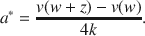
5.2 Interaction effects
Is it possible that difficulty mediates the effects of monetary rewards and cost? To explore this possibility, I compute the ATEs of bonus, wage, and cost at different values of difficulty and plot them on Fig. 4. The figure shows that higher difficulty in general increases the treatment effects of the monetary variables but in many cases this interaction is too small to be statistically significant. In particular, increasing difficulty from 0 to 1 increases the ATE (reduces the negative ATE) of cost by 0.03 (p-value
 , t-test), increases the ATE of wage by 0.04 (p-value
 , t-test), and increases the ATE of bonus by 0.08 (p-value
 , t-test).Footnote 23 Hence the data suggest that conditional rewards are most effective in stimulating effort when difficulty is high. This result is consistent with Vandegrift and Brown (Reference Vandegrift and Brown2003) who also find that conditional rewards are more effective on difficult tasks.
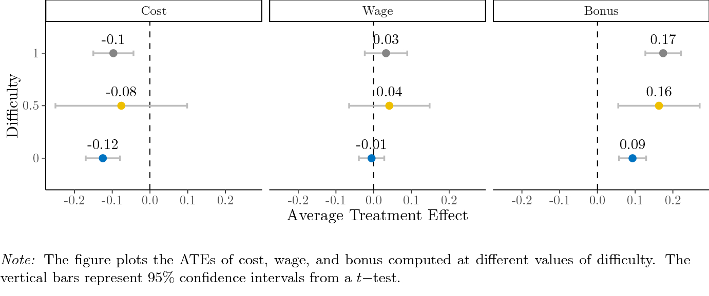
Fig. 4 ATEs Conditional on Difficulty
5.3 Structural analysis
In this section I ask whether a simple structural model can explain the observed behavioral patterns. As highlighted by the theoretical analysis in Sect. 4, the inverse-U pattern of effort response to difficulty can be accommodated by the model with probability weighting, but not by the EU model.
5.3.1 Estimation procedures
Consider an agent with preferences
 who faces treatment
 . The utility of effort choice
 will be given by

where
 ,
,
 is the probability weighting function parametrized by
 , and
, and
 is the utility function parametrized by
 . In the experiment, the utility function u is
 . The cost function c and the probability of success function p are defined by equations (2) and (1), respectively.
I assume that
 takes the two-parameter Prelec form (Prelec Reference Prelec1998), which is frequently used in applied work (Wilcox Reference Wilcox2015a; l’Haridon and Vieider Reference l’Haridon and Vieider2019) and has been shown to have good empirical properties (Stott Reference Stott2006), with
 . Parameter
 determines the shape of the function, while parameter
 determines the scale of the function.

where
 . I also assume that v takes the standard constant relative risk aversion (CRRA) form, with


I estimate a representative agent model on the pooled data and use i to index individual observations. In each observation i, effort is assumed to be chosen to maximize
 , where
 is an observed vector of treatment variables, which in the present case is an equivalent of regressors in a reduced-form model,
 is an unobserved vector of preference parameters, to be estimated, and effort a is the outcome variable. The optimal effort as a function of the treatment variables vector
 and the preference parameter vector
 is denoted
 . No closed-form expression for
 exists a model specification given by (8), (9), and (10), therefore, I rely on a numerical solution for optimal effort. I assume that the observed effort follows

where
 is a mean-zero error term. To estimate the model, I use a non-linear least squares estimator,Footnote 24 which minimizes the sum of squared deviations between the observed and predicted choices:
The risk-neutral parameter vector
 is used as a starting value.
5.3.2 Estimation results
Table 4 presents the estimation results. The estimates show that subjects are moderately risk averse in terms of the contribution of the curvature of the utility function to risk aversion. This finding is consistent with the previous findings in the laboratory experiments (Holt and Laury Reference Holt and Laury2002; Andersen et al. Reference Andersen, Harrison, Lau and Rutström2008), however the estimate for the CRRA parameter is higher than is typically reported for binary lottery choices (Harrison and Rutström Reference Harrison and Rutström2008)[P. 121]. The 95% confidence interval for
 covers the value of one, which implies a special case of a logarithmic utility.
Table 4 Estimates of the model with Probability Weighting

|
Parameter |
Estimate |
SE |
2.5% |
97.5% |
|---|---|---|---|---|
|
|
0.978 |
0.117 |
0.748 |
1.208 |
|
|
1.603 |
0.071 |
1.464 |
1.743 |
|
|
0.821 |
0.054 |
0.716 |
0.926 |


N obs = 1625
The table reports the estimation results of the model specified in Eqs. (8), (9), and (10). The table reports the point estimates, standard errors, as well as 95% confidence intervals. The estimated parameters are the risk aversion (
 ), the shape parameter of the probability weighting function (
 ), and the scale parameter of probability weighting function (
 )
)
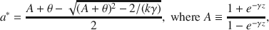
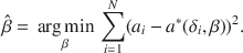
The estimate of
 , which determines the shape of the probability weighting function, is significantly greater than one and leads to an S-shaped probability weighting. The S-shaped probability weighting implies likelihood sensitivity: subjects underweight the likelihoods of rare outcomes. As highlighted by the theoretical analysis in Sect. 4, such a shape arises precisely to fit the inverse-U pattern of effort response to difficulty that is observed in the data. The estimate of the scale parameter
 is different from 1, which implies that the probability weighting function crosses the diagonal at a point other than 1/e. Specifically, when
 the crossing point is
 , which for the given estimates yields a value of
 .
.
Figure 5 (left panel) shows the estimated probability weighting function,
 . The underweighting occurs for probabilities approximately less than 0.25. Probabilities greater than 0.25 are overweighted. The right panel of Fig. 5 shows the implied decision weights from the estimated probability weighting function. The decision weights are computed using equiprobable lotteries with different number of outcomes (two, three, or four).Footnote 25 The picture shows that extreme outcomes are underweighted when there are more than two outcomes, and the worst (best) outcome is underweighted (overweighted) when there are exactly two outcomes.
The estimated shape of the weighting function is in stark contrast with some of the previous estimates (Wu and Gonzalez Reference Wu and Gonzalez1996; Bruhin et al. Reference Bruhin, Fehr-Duda and Epper2010; l’Haridon and Vieider Reference l’Haridon and Vieider2019) that report an inverse-S shaped probability weighting function first proposed by Kahneman and Tversky (Reference Kahneman and Tversky1979).Footnote 26 While an inverse-S-shaped weighting function leads to overweigthing of small probabilities, I find underweighting of small probabilities. Interestingly, underweighting of small probabilities in a labor context was reported recently by DellaVigna and Pope (Reference DellaVigna and Pope2018) who find that subjects significantly underweight a 1% chance of winning the prize. Their estimates indicate that subjects perceive 1% as 0.2–0.38%, depending on the estimated model. My estimates, however, imply a more extreme underweighting: a 1% chance of receiving a prize is perceived as only 0.007%. The present results are also related to the results reported by Wilcox (Reference Wilcox2015b) in a lottery-choice context. The study finds that the second most common type of probability weighting (after the concave shape) is also S-shaped.
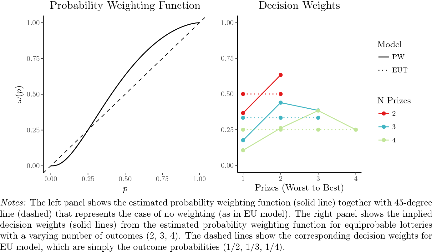
Fig. 5 Estimated probability weighting function and implied decision weights
Figure 6 compares the predicted effort,
 , from the estimated model, specified in Eqs. (8), (9), and (10), to the actual effort,
 , split by treatment variable. The figure shows that the estimated model reproduces the comparative statics found in the data reasonably well.Footnote 27 In particular, the model does capture the inverse-U pattern of effort response to difficulty. It over-predicts, however, the mean effort for
 leading to a more prolonged increase in effort as difficulty increases and a sharper drop in effort when difficulty changes from 0.75 to 1. The estimated model generates somewhat larger changes in effort in response to changes in wage, bonus, and cost than observed in the data.
Fig. 6 Actual and predicted mean effort levels
5.4 Alternative explanations
Is it possible that the observed inverse-U pattern of effort response to difficulty is generated via a mechanism other than probability weighting? To consider this possibility, one has to re-examine the comparative statics result (5). The result shows that the effect of difficulty on effort is determined by the signs of the two cross-partial derivatives,
 and
and
 .Footnote 28 Consider first the cross-partial derivative of the utility function,
 . In the experiment, the cost of effort is induced to be monetary, hence the utility function can be written as
 . The cross-partial derivative is then given by
 . Assuming risk-aversion, the sign of this derivative is positive.
Suppose, however, that subjects somehow misinterpret the cost of effort function or have a non-standard utility function. Even if subjects perceive the cost function to be
 instead of the induced
 , this would not change the result since it is unlikely that the perceived cost function would ever be decreasing. Subjects could clearly observe that higher effort resulted in more, rather than less, costs. Moreover, the first-derivative of
 would need to change its sign with difficulty to generate a non-monotonic effect of difficulty, which again is unlikely in the present design.
Suppose, on the other hand, that subjects’ utility-of-money function v is non-concave. A convex function v (i.e., risk-loving) would result in a positive cross-partial derivative and a monotonically increasing response to difficulty, not the observed inverse-U response. The utility-of-money function can be even more complex. For example, it can be convex for outcomes below a certain reference point and concave for outcomes above the reference point, resulting in an S shape as in the CPT value function (Tversky and Kahneman Reference Tversky and Kahneman1992). In this case the second derivative of v would change its sign, and hence, the effect of difficulty would vary: difficulty would have a positive effect on effort for relatively low monetary outcomes and a negative effect for relatively high monetary outcomes. Note, however, that the sign of the effect of difficulty would not vary with difficulty itself. The implication of this alternative assumption is that the observed non-monotonic effect of difficulty is actually confounded with the effect of monetary rewards. In this case the low-difficulty treatments should have been administered for low monetary rewards and the high-difficulty treatments should have been administered for high monetary rewards. This is impossible in the present design since the values of difficulty and monetary rewards were assigned independently. The distribution of observations between
 and
and
 (50/50) is exactly the same for low and high values of w and for low and high values of z. Figure D.3 in Appendix D.1 further rejects the assumption of an S-shaped function v by showing that the inverse-U effect of difficulty is observed both for low and high levels of monetary outcomes.
Consider next the cross-partial derivative of the probability of success function,
 . The probability of success function is induced to be linear, hence, its cross-partial derivative is zero.Footnote 29 This leaves us with the only possibility that subjects perceive the probability of success to be
 instead of p, i.e., they must use probability weighting.Footnote 30
6 Conclusion
Research in labor economics has traditionally focused on monetary rewards as the primary incentive tool for principals to incentivize agents. Research in behavioral economics shows that monetary rewards are subject to psychological factors and that alternative behavioral incentives are also relevant for building incentive schemes for agents. I contribute to this strand of behavioral economics by drawing upon the insights of a prominent psychological theory of motivation, motivational intensity theory. Motivational intensity theory argues that the primary determinant of effort is task difficulty.
I study the effect of task difficulty and monetary rewards on effort in an incentivized experiment. I find that difficulty has an inverse-U effect on effort: effort first increases as difficulty goes up, reaches a peak, and then drops as difficulty continues to increase. The magnitude of the incentive effect of difficulty is on par with the magnitude of the incentive effect of conditional monetary rewards. Difficulty mediates the effect of monetary rewards: conditional rewards are most effective at inducing effort when task difficulty is intermediate or high.
The benefit of the present design is that it allows for a clean test of a particular mechanism behind the effect of task difficulty on effort: probability weighting. It is possible that in natural work environments the effect of difficulty on effort works through various other mechanisms, such as choking under pressure (Ariely et al. Reference Ariely, Gneezy, Loewenstein and Mazar2009; Hickman and Metz Reference Hickman and Metz2015). Likewise, it is possible that in the present chosen effort framework subjects are learning to optimize a model, and that the response to difficulty in a real effort framework, in which the probability of success function is not induced, would be different and, in particular, depend on subjects’ ability. It is of interest, therefore, to investigate these alternative potential mechanisms and frameworks, as well as their interaction with the proposed mechanism, in future studies.
The structural estimates of the model yield an S-shaped probability weighting function. These estimates are different from the estimates in previous studies, which typically find an inverse-S-shaped probability weighting function. The first possible explanation for such a difference is that the present experiment is framed in a labor context, while previous studies typically used an abstract lottery context. Contextual instructions can affect subjects’ behavior, as is evident from a variety of studies (Harrison and List Reference Harrison and List2004; Alekseev et al. Reference Alekseev, Charness and Gneezy2017). This explanation is consistent with the recent evidence in DellaVigna and Pope (Reference DellaVigna and Pope2018) who report underweighting of small probabilities in a field experiment on effort. However, this explanation raises the follow-up question that would deserve further investigation: what features of a labor context make it different from an abstract context.
Another difference between the present study and previous studies on lottery tasks is the frequency of feedback. In the effort task, the feedback is provided every round, while in the lottery tasks, the feedback is typically provided only after all the choices are made. Experimental evidence suggests that providing frequent feedback can make subjects more sensitive to probabilities. Frequent feedback has been shown to result in linear probability weighting (Van de Kuilen Reference Van de Kuilen2009), or even in S-shaped probability weighting (Hertwig et al. Reference Hertwig, Barron, Weber and Erev2004; Hertwig and Erev Reference Hertwig and Erev2009) in a binary lottery choice setting.
The present findings are relevant for the design of optimal incentive schemes for workers and modeling effort. The strong incentive effect of difficulty calls for taking it into account when assigning tasks to workers. A manager can expect that it will take workers more effort to complete a moderately hard task than an easy task. However, a very hard task might not be devoted as much effort as desired.Footnote 31 This behavioral response amplifies the direct negative effect of difficulty and thus can substantially lower a worker’s performance. A principal can counter this detrimental behavioral effect of difficulty using conditional rewards since they are found to be most effective when difficulty is high. From a theoretical perspective, my results suggest that supplementing the workhorse model of effort with probability weighting can better explain certain patterns of effort provision and yield higher predictive power. From a methodological perspective, the present results suggest that experimental designs should control for difficulty to avoid confounding and that researchers can exploit the interaction between task difficulty and incentives to avoid a “ceiling-effect” problem.
Funding
Open Access funding enabled and organized by Projekt DEAL.


 Open access