


1 Introduction
SCR-1 is a small modular stellarator designed, built and implemented at Instituto Tecnológico de Costa Rica. During its initial stage, the main goal of the SCR-1 project was to understand and overcome the engineering challenges related with the construction of a small fusion device (Vargas et al. Reference Vargas, Mora, Otárola, Zamora, Asenjo, Mora and Villalobos2015). However, the first hydrogen discharge in 2016 (similar to the discharge shown in figure 1) pointed out the start of the current stage of the project, devoted to the study of the physics involved in SCR-1. This work presents the latest results in diagnostics implementation, heating simulation and magnetohydrodynamics (MHD) calculations.
1.1 SCR-1 parameters
The SCR-1 main parameters are the following (Solano-Piedra et al. Reference Solano-Piedra, Vargas, Köhn, Coto-Vílchez, Sanchez-Castro, López-Rodríguez, Rojas-Quesada, Mora and Asenjo2017).
(i) Two field period modular stellarator.
(ii) Major radius
 $R=247.7~\text{mm}$.
(iii) Aspect ratio
$=$ 6.2.(iv) Low-shear configuration.
(v)
$\unicode[STIX]{x1D704}_{0}=0.312$ and $\unicode[STIX]{x1D704}_{a}=0.264$.(vi) 6061-T6 aluminium vacuum vessel.
(vii) ECH power 5 kW (2.45 GHz), second harmonic (
$B=43.8~\text{mT}$), $\langle \boldsymbol{B}\rangle =41.99~\text{mT}$.(viii) 12 modular coils with six turns each.
(ix) Current of 725 A per turn, with a toroidal field (TF) current of 4.35 kA-turn per coil.
(x) The coils are powered by a cell battery bank of 120 V.
(xi) Plasma pulse 4–10 s.


1.2 Plasma parameters
Plasma in SCR-1 has the following parameters (Solano-Piedra et al. Reference Solano-Piedra, Vargas, Köhn, Coto-Vílchez, Sanchez-Castro, López-Rodríguez, Rojas-Quesada, Mora and Asenjo2017).
(i) Minor plasma radius:
$39.95~\text{mm}$.(ii) Line-averaged electron density:
$5\times 10^{16}~\text{m}^{-3}$.(iii) Plasma density cut-off value:
$7.45\times 10^{16}~\text{m}^{-3}$.(iv) Estimated energy confinement time:
$5.70\times 10^{-4}~\text{ms}$.(v) Plasma volume:
$0.0078~\text{m}^{3}$.(vi)
$\unicode[STIX]{x1D6FD}_{\text{Total}}=0.01\,\%$.(vii) Electron temperature: 6–14 eV.


2 Diagnostics
Since 2016, three diagnostics have been operating in SCR-1: a Langmuir probe, an optical spectrometer and a fast camera (Mora et al. Reference Mora, Vargas, Asenjo, Barillas, Coto-Vílchez, Esquivel-S, Solano-Piedra, Otárola, Villalobos and Gatica-Valle2016). However, in order to expand the plasma studies and heating scenarios, new diagnostics were designed recently and are currently being implemented. The aforementioned diagnostics are a bolometer (discussed in § 2.1) and magnetic diagnostics (discussed in § 2.2). With these two new diagnostics, we look forward to improving the understanding of the phenomena taking place in SCR-1. Both diagnostics will be positioned in the highlighted locations shown in figure 2.

Figure 1. SCR-1 hydrogen plasma discharge.

Figure 2. SCR-1 upper view with highlighted toroidal positions.
2.1 Bolometer
A bolometer was designed to measure the total radiated power by the plasma in the SCR-1 device. The functional principle of the bolometer is to capture the radiation emission from SCR-1 using an AXUV20EGL 20-element photodiode array. The emissivity of the plasma is determined by using the electron temperature and density profiles. Then, they are integrated for each chord to construct a synthetic diagnostic that will be compared with experimental results. These chords are presented in figure 3. The bolometer for SCR-1 will be installed in  $150^{\circ }$ toroidal position (see figure 2). The photodiodes feature a nearly flat spectral responsivity of
  $R_{o}\approx 0.275~\text{A}~\text{W}^{-1}$ for photon energies of 0.2–
 $5~\text{keV}$. The quantum efficiency loss (mainly for 7–100-eV photons) is due to the front radiation-hard silicon dioxide window since oxide absorption and reflections are not negligible. Finally, the spatial resolution of the bolometer is
  $0.8~\text{mm}$ and the temporal resolution is 200 ns.

Figure 3. Chord geometry for the bolometer array and plasma equilibrium for synthetic discharge.
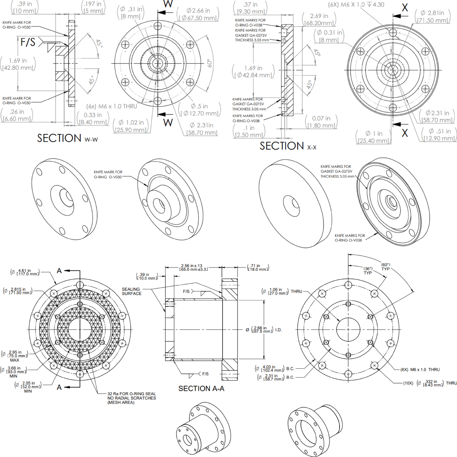
Figure 4. Layout and technical drawing of bolometer case and pinhole case.
Regarding the case, it was designed based on the cylindrical geometry of the ports of SCR-1 as shown in figure 4. The dimensions of the ports are 83.13 mm and 72.9 mm, depth and diameter, respectively. The case itself has three cylindrical pieces made of stainless steel, all with different diameters and joined by welding. Additionally, the case has holes to couple it with the SCR-1 ports through bolts. Finally, knife marks for fluorocarbon gaskets were included in the case, to guarantee the high-vacuum conditions inside the vessel.

Figure 5. Bolometer mechanical design (exploded view).
In figure 5, the pinhole lid is a metallic structure that regulates the radiation stream of light towards the photodiode. The lid structure consists of a stainless steel sheet with a diameter of  $41.92~\text{mm}$ and a pinhole with a diameter of
  $0.8~\text{mm}$. This pinhole allows the radiation to hit the photodiode array and, consequently, measures the radiation energy emitted by the plasma. Since the pinhole lid is an independent part, it can be replaced with different diameters to perform different tests without any modification in the structure. The pinhole lid is attached to the sapphire uncovered wedged lens that has a diameter of
  $25.4~\text{mm}$ and a thickness of
  $5~\text{mm}$; the wavelength range of the lens is between 150 nm and
  $4.5~\unicode[STIX]{x03BC}\text{m}$.
The design is shown in figure 4, including all the parts to be assembled. The pinhole lid and the lens are enclosed by two metallic cases, front and rear. The assembly between metallic parts requires gaskets due to high-vacuum requirements. All the measurements in the design have specified tolerances according to the ISO 128 standard.
An electronic system for the bolometer has been designed. The printed circuit board has a four-layer design and its diameter is  $65.0~\text{mm}$. This design includes the photodiode array in photoconductive mode, the transimpedance amplifiers (TIAs) and filters for signal conditioning. The photodiode array chip is an AXUV20ELGDS (20 elements). For the TIAs, the selected operational amplifiers (OPAMs) are OPA4350. The chosen amplifier exhibits low input bias currents, ample frequency bandwidth and low input offset voltages. Although the circuit looks quite simple, hidden parasitics can cause unwanted circuit instability. The AC signal gain is dependent on the feedback components. Equation (2.1) shows how the output voltage depends on the various parameters of the bolometer:
 $$\begin{eqnarray}V_{\text{out}}=I_{pd}\frac{R_{f}}{1+SR_{f}C_{f}},\end{eqnarray}$$
 where  $I_{pd}$ is the photodiode ‘dark current’,
  $R_{f}$ is the feedback resistor,
  $S$ represents the single-pole frequency response, and
  $C_{f}$ is the feedback capacitor.
Noise gain is an important factor and the intersection point between the amplifier open-loop gain and the noise gain defines the stability of the circuit. The recommended phase margin is  $45^{\circ }$ producing a 23 % overshoot step response, which represents a stable operation.
Finally, an electromechanical system is under development to auto-calibrate the exact position of the photodiode. This calibration allows us to maximize the measurements of radiation coming out from the stellarator. This flexible design allows the use of the bolometer in devices where the distance between the photodiode and the pinhole may change.
2.2 Magnetic diagnostics
Magnetic diagnostics are currently under development for SCR-1. Specifically, two sets of Rogowski coils are being developed to measure toroidal plasma current, two sets of diamagnetic loops to measure plasma energy content and three sets of Mirnov coils to observe magnetohydrodynamic modes.
These three diagnostics follow the same operating principle: induced current associated to a voltage. This voltage is related to a magnetic signal according to a calibrating system. This system consists of Helmholtz coils for which the magnetic signal is known using magnetic sensors (Pasco CI-6520A) and thus the output voltage in the diagnostic when exposed to the Helmholtz field is related to magnetic field intensity. Relatively small currents and short pulses are the main limitation in the making of these magnetic diagnostics. Moreover, the small vacuum vessel makes their placement a challenging task.

Figure 6. Amplifier–integrator circuit for the Rogowski coil.
2.2.1 Rogowski coils
Rogowski coils are going to be located close to the bolometer port, both inside and outside the vessel. The Rogowski diagnostic is essentially a toroidal solenoid placed around the plasma volume aiming to register the magnetic flux passing through the solenoid interior. This Rogowski coil is expected to measure signals coming from currents of 0.1–1.0 A. A rough estimation of the sensitivity of approximately  $0.2~\text{V}~\text{s}~\text{A}^{-1}$ was determined. In the case of the Rogowski coils, the expression for the integrated signal is presented in (2.2):
 $$\begin{eqnarray}V_{0}=\int V_{\text{rog}}\,\text{d}t=\int \left(\frac{\text{d}\unicode[STIX]{x1D6F7}_{B}}{\text{d}t}\right)\text{d}t=\frac{a^{2}\unicode[STIX]{x1D707}_{0}N}{2R}I_{p}(t)+\text{const.},\end{eqnarray}$$
 where  $a$ is the Rogowski loop radius,
  $R$ is the radius of the cylindrical–toroidal coordinate system,
  $N$ is the number of loops and
  $I_{p}$ is the toroidal current to be integrated in time.
An analytical simplified expression taken from Boozer & Gardner (Reference Boozer and Gardner1990) was used to estimate the magnitude order for the bootstrap current,
 $$\begin{eqnarray}I_{BS}\approx 1.46\frac{\sqrt{\unicode[STIX]{x1D716}}}{\unicode[STIX]{x1D704}}\approx 0.5~\text{A},\end{eqnarray}$$
 where  $\unicode[STIX]{x1D716}$ is the inverse of the aspect ratio and
  $\unicode[STIX]{x1D704}$ the rotational transform.
This calculation was made in order to construct the amplifier–integrator circuit of the Rogowski coil presented in figure 6. The integrating phase of this circuit limits the DC gain by using a resistance in parallel to the capacitor. The cut-off frequency was estimated to be around 160 Hz. The amplifier part of the circuit uses a potentiometer to adjust the gain according to the experimental values of measurements. The use of a compensation resistance is proposed to reduce the effect of the bias current.
The Rogowski coil will be wound around a ring of material with  $\unicode[STIX]{x1D707}_{r}\approx 1$ with 20 cm of internal diameter, 22 cm of external diameter and around 60 turns. A return ground conductor around the core of the coil will be wound to avoid spurious inductive signals. So far, tests are carried out using ad hoc signals. For instance, a Rogowski coil prototype is placed encircling a variable current leading cable, testing the responsiveness of the integrating circuit and the diagnostic itself. Further characterization of the diagnostic wires and insulation material choosing are still pending. Data acquisition and processing will take place in a future stage of the project, as well as in situ tests.

Figure 7. Rotational transform, magnetic shear and well depth profiles at  $0^{\circ }$ toroidal angle.
2.2.2 Diamagnetic loops and Mirnov coils
Diamagnetic loops will be located at  $0^{\circ }$ and
  $90^{\circ }$ on the toroidal axis angles (see figure 2), outside and inside the vacuum vessel. On the other side, Mirnov coils will be at
  $0^{\circ }$,
  $45^{\circ }$ and
  $90^{\circ }$ on the toroidal axis angles (see figure 2), with a total of 10 turns each. The exact poloidal distribution of each set of the Mirnov diagnostics is not relevant in this first experimental stage, for which the only objective is to obtain reliable magnetic measurements. More pertinently, information regarding MHD modes and the characterization of the magnetic topology (information that is not known) are needed to optimally place the Mirnov coils.
3 MHD and heating
3.1 MHD equilibrium calculations
The calculations of the MHD equilibria for the SCR-1 stellarator were performed by VMEC (see below) in free-boundary mode. As results of these calculations, the rotational transform ( $\unicode[STIX]{x1D704}$) for
  $0^{\circ }$ toroidal position, magnetic well and magnetic shear profiles were obtained and shown in figure 7. The decrease of the rotational transform with the effective radius indicates that the outer magnetic flux surfaces bend more sharply than inner magnetic flux surfaces. Similarly, magnetic shear is shown to be more negative with an increase in the effective radius for low-
 $\unicode[STIX]{x1D6FD}$ plasma. Hence, it is possible to recognize a plasma region where the propagation of electron drift waves is stable (Nadeem, Rafiq & Persson Reference Nadeem, Rafiq and Persson2001) due to the low-
 $\unicode[STIX]{x1D6FD}$ nature of SCR-1. Finally, the negative and decreasing magnetic well values towards the plasma edge suggest the presence of significant fluctuations. This behaviour is observed in devices like TJ-II, as reported by Castellano et al. (Reference Castellano, Jiménez, Hidalgo, Pedrosa, Fraguas, Pastor, Herranz and Alejaldre2002), and, with experimentation in SCR-1, we look forward to confirming that same behaviour.
On the other hand, vacuum magnetic flux surface mapping was computed using a modified oscillating rod with ZnO:Zn phosphor (Coto-Vílchez et al. Reference Coto-Vílchez, Vargas, Barillas, Sánchez-Castro, Queral, Vílchez-Coto, Cerdas, Asenjo, Mora and Zamora-Picado2017). The mapped surfaces were compared with the calculations obtained using BS-SOLCTRA code (the plots are displayed in figure 8). These comparisons show that calculations and measurements are consistent with each other, as shown in figure 9. Therefore, these results suggest that the manufacturing process was correct and indicate that the magnetic field in SCR-1 behaves as expected. Further measurements will allow us to calculate more surfaces and consequently refine results.

Figure 8. Vacuum magnetic flux surfaces calculated with BS-SOLCTRA at toroidal positions of (a)  $0^{\circ }$, (b)
  $45^{\circ }$ and (c)
  $90^{\circ }$.

Figure 9. Comparison between surfaces: (a) mapping and (b) calculations.
Particle tracing simulations were obtained using BS-SOLCTRA code (Vargas et al. Reference Vargas, Kohn, Meneses, Jiménez, Garro-Vargas, Solano-Piedra, Coto-Vílchez, Rojas-Quesada, López-Rodríguez and Sánchez-Castro2018), a code written specifically for SCR-1 in Matlab and then migrated to C++ for the visualization of the 3D vacuum magnetic field lines and magnetic flux surfaces (Jiménez et al. Reference Jiménez, Campos-Duarte, Solano-Piedra, Araya-Solano, Meneses and Vargas2020). This model calculates the trajectory of particles due to the SCR-1 coils using Biot–Savart fields of a filamentary segment, under the consideration that particle motions are independent of each other. A scientific visualization tool called Paraview (Solano-Piedra et al. Reference Solano-Piedra, Vargas, Köhn, Coto-Vílchez, Sanchez-Castro, López-Rodríguez, Rojas-Quesada, Mora and Asenjo2017) was used to generate the last closed magnetic flux surface and visualize the trajectories of particles, as shown in figure 10. Both the BS-SOLCTRA code and the implementation of Paraview work as a parallelized magnetic plasma confinement simulation framework (Jiménez et al. Reference Jiménez, Campos-Duarte, Solano-Piedra, Araya-Solano, Meneses and Vargas2020).

Figure 10. Last close magnetic flux surface visualization.
3.2 Microwave heating simulations
In the case of SCR-1, the WKB method (ray tracing) was discarded because the density length scale  $\unicode[STIX]{x1D735}n_{e}/n_{e}\approx 0.01~\text{cm}$ is small in comparison with the wavelength of the incident wave (
 $\unicode[STIX]{x1D706}_{0}=12.45~\text{cm}$). Therefore, the microwave heating scenarios were simulated using the IPF-FDMC full-wave code (Köhn et al. Reference Köhn, Jacquot, Bongard, Gallian, Hinson and Volpe2011). This code solves Maxwell’s equations for a grid in order to calculate the maximum single-pass percentage of the ordinary waves (O waves) to extraordinary waves (X waves) conversion, as described in Hansen et al. (Reference Hansen, Lynov, Maroli and Petrillo1988). The O–X conversion scheme can be identified due to the perturbations of the root mean square field located near the upper hybrid resonance (UHR). In the case of the conversion from X waves to Bernstein waves (B waves), the X waves can either be fully converted into Bernstein mode or get damped by collisional ion–electron damping in regions around the UHR (Laqua Reference Laqua2007). Then, the percentage of O–X conversion determines the overall O–X–B conversion process as long as the X–B conversion is different from zero. In this case, the calculations were made for the
  $330^{\circ }$ toroidal position. The input parameters of the full-wave code were the electron density and vacuum total magnetic field contour map for this position. The radial electron density profile (presented in figure 11) was plotted using (3.1):
 $$\begin{eqnarray}n(r_{\text{eff}})=n_{0}\exp -\left(-\frac{r_{\text{eff}}}{w_{n}}\right)^{\unicode[STIX]{x1D6FC}_{n}},\end{eqnarray}$$
 where  $w_{n}=0.0249826$ and
  $\unicode[STIX]{x1D6FC}_{n}=4$ were the input parameters, while
  $n_{0}$ was the value of the line-averaged electron density on the magnetic axes presented in § 1.2.

Figure 11. Electron density and magnetic field strength contour map for the toroidal position at  $330^{\circ }$.

Figure 12. Magnetic field strength contour map for the toroidal position at  $330^{\circ }$.
The magnetic field profile for the selected toroidal position (shown in figure 12) was created with magnetic field values calculated by the XGRID module for the equilibrium solver VMEC (provided by IPP at Greifswald) and the magnetic flux surfaces, calculated using VMEC as well.
The value of the angle between incident electromagnetic waves and external magnetic field for optimum O–X conversion was approximately  $58^{\circ }$ in poloidal direction, estimated by (3.2):
 $$\begin{eqnarray}\unicode[STIX]{x1D703}_{\text{opt}}=\arccos \left(\frac{Y}{Y+1}\right),\end{eqnarray}$$
with
 $$\begin{eqnarray}Y={\displaystyle \frac{\unicode[STIX]{x1D714}_{0}}{\unicode[STIX]{x1D714}_{ce}}},\end{eqnarray}$$
 where  $\unicode[STIX]{x1D714}_{0}$ is the frequency of the incident radiation and
  $\unicode[STIX]{x1D714}_{ce}$ is the electron cyclotron frequency.
An enhancement of the magnitude of the electric field wave was found in the vicinity of the upper hybrid resonance for the first microwave heating scenario. This scenario considers the plasma heating at the second harmonic of the magnetic field (see figures 13 and 11), where the X wave, generated by the O–X conversion, was numerically damped in the code. Since the overall O–X–B mode conversion efficiency is determined by the O–X conversion efficiency, it was found that the microwave heating scenario showed that the O–X–B conversion efficiency was around 12–14 % with an optimum size beam of  $1.1\unicode[STIX]{x1D714}_{0}$. The full-wave code implemented a Gaussian microwave beam, which integrates a time-harmonic field to one component of the propagating waves. This beam propagates in one direction, as is presented in (3.4):
 $$\begin{eqnarray}E_{z}=A(t)E_{0}\exp \left(\frac{x-x_{0}}{w_{\text{gauss}}}\right),\end{eqnarray}$$
 where  $A(t)$ changes between 0 and 1,
  $E_{0}$ is the amplitude of the electric field,
  $x_{0}$ is the centre of the Gaussian beam and
  $w_{\text{gauss}}$ is the beam waist. The Gaussian beam is similar to the one presented in Kön et al. (Reference Köhn, Cappa, Holzhauer, Castejón, Fernández and Stroth2008).

Figure 13. Full-wave simulations at the  $330^{\circ }$ toroidal position for the injection angle of
  $58^{\circ }$ after 20 periods of oscillation.

Figure 14. Full-wave simulations at the  $330^{\circ }$ toroidal position for the injection angle of
  $58^{\circ }$ after 20 periods of oscillations. The magnitude of the magnetic field was reduced to its fourth harmonic.
The second heating scenario was obtained from a different magnetic field profile, where the plasma of SCR-1 will be heated in the fourth harmonic of the magnetic field. The electron density profile of the first scenario and the launching angle were maintained. Figure 14 shows oscillations of the electric field throughout the plasma region, where peaks exist in interior regions of the plasma core, compared to the first microwave scenario. It is important to notice that no clear region is defined for the upper hybrid frequency or the O mode cut-off frequency. As expected, the decrease in the magnitude of the total magnetic field allows a shift of the place of the upper hybrid frequency, which indicates that there is no central heating (Nagasaki & Yanagi Reference Nagasaki and Yanagi2002). This second microwave heating scenario has an O–X–B conversion of around 0–1 %.
4 Conclusions
New diagnostics are being implemented in SCR-1. A bolometer placed in a stainless steel case was designed with an adjustable autocalibration system that allows its use in other devices if necessary. The designs for the magnetic diagnostics are finished and its toroidal positions are well defined. However, it is still pending to define the exact poloidal distribution of the Mirnov coils. In total, seven different sets of magnetic diagnostics are expected to be implemented. Mapping results confirm that the magnetic field inside the device behaves as expected in the calculations. Such mapping suggests that the device was correctly built. The electron Bernstein waves could be damped by ion–electron collisions; therefore, it is necessary to know the ion density profile for the plasma of SCR-1 in order to calculate the ion–electron collision frequency.
Editor Per Herlander thanks the referees for their advice in evaluating this article.


